Spatial-Temporal Variations of Summertime Ozone Concentrations across a Metropolitan Area Using a Network of Low-Cost Monitors to Develop 24 Hourly Land-Use Regression Models

Abstract

Ten relatively-low-cost ozone monitors (Aeroqual Series 500 with OZL ozone sensor) were deployed to assess the spatial and temporal variability of ambient ozone concentrations across residential areas in the Monroe County, New York from June to October 2017. The monitors were calibrated in the laboratory and then deployed to a local air quality monitoring site where they were compared to the federal equivalent method values. These correlations were used to correct the measured ozone concentrations. The values were also used to develop hourly land use regression models (LUR) based on the deletion/substitution/addition (D/S/A) algorithm that can be used to predict the spatial and temporal concentrations of ozone at any hour of a summertime day and given location in Monroe County. Adjusted R² values were high (average 0.83) with the highest adjusted R² for the model between 8 and 9 AM (i.e. 1–2 hours after the peak of primary emissions during the morning rush hours). Spatial predictors with the highest positive effects on ozone estimates were high intensity developed areas, low and medium intensity developed areas, forests+shrubs, average elevation, Interstate+highways, and the annual average vehicular daily traffic counts. These predictors are associated with potential emissions of anthropogenic and biogenic precursors. Maps developed from the models exhibited reasonable spatial and temporal patterns, with low ozone concentrations overnight and the highest concentrations between 11 AM and 5 PM. The adjusted R² between the model predictions and the measured values varied between 0.79 and 0.87 (mean = 0.83). The combined use of the network of low-cost monitors and LUR modelling provide useful estimates of intraurban ozone variability and exposure estimates that will be used in future epidemiological studies.

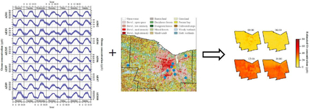
Graphical abstract

1. Introduction

In the troposphere, ozone (O₃) is a secondary air pollutant generated through a series of complex photochemical reactions involving solar radiation and ozone-precursors, e.g., reactive nitrogen oxides (NO_y), carbon monoxide (CO), and reactive volatile organic compounds (VOCs) of biogenic and anthropogenic origin (e.g., Monks, 2005; Stevenson et al., 2013; Cooper et al., 2014; Monks et al., 2015; Seinfeld and Pandis, 2016). Tropospheric O₃ is known to be harmful to human health (Jerrett et al., 2009; Bell et al., 2014; Turner et al., 2016) and ecosystems (Fowler et al., 2009; Ainsworth et al., 2012). The Global Burden of Disease Study 2010 (Lim et al., 2012) estimated almost 2.5 million worldwide disability-adjusted life years attributable to ozone in 2010. In addition, premature deaths were also associated with long-term exposure to ozone (Jerrett et al., 2005). However, the size and the consistency of the association between ozone exposure and health effects vary, and this uncertainty may arise from inaccurate exposure assessment (Jerrett et al., 2013; Wolf et al., 2017) since the exposure assessments are typically based only on community-scale average concentrations (Jerrett et al., 2005).

During recent decades, mitigation strategies have been implemented across North America to improve the air quality at both federal and state levels (e.g., Gerard and Lave, 2005; Parrish et al., 2011; Squizzato et al., 2018). These strategies aimed to regulate and thereby reduce the anthropogenic emissions of key primary air pollutants, including ozone precursors (NO_x, VOCs), sulfur dioxide (SO₂), and particulate matter (PM). Since 2000, mitigation regulations have required reduced emissions from light- and heavy-duty vehicles, maritime transport, and electric power generation resulting in decreased air concentrations for most air pollutants (e.g., Parrish et al., 2011; Pouliot et al., 2015; Duncan et al., 2016; Emami et al., 2018; Masiol et al., 2018a). However, ozone concentrations have shown a different behavior. Squizzato et al. (2018) showed that the decreased NO_x emissions contributed to the reduction of ozone formation during the summer, but it did not reduce the spring maxima across New York State (NYS). Furthermore, O₃ concentrations increased during the autumn and winter at multiple monitoring sites in NYS (Squizzato et al., 2018).

In the U.S., air quality (AQ) is managed through National Ambient Air Quality Standards (NAAQS). NAAQS determine the limit values for the protection of public health (primary standard) and public welfare (secondary standard) of six “criteria” air pollutants, including ozone. Concentrations of ozone are measured using federal “reference” or “equivalent” methods (FRM and FEM, respectively) in accordance with Code of Federal Regulations (40 CFR Part 53; USEPA, 2017). Compliance with NAAQS is routinely evaluated at one or a few stationary urban stations that are used to assess the exposure of the whole population living in that metropolitan area. However, the spatial coverage of the monitoring network is likely to be insufficient to capture the intraurban spatial variability of ozone concentration, resulting in inaccurate exposure assessments. Ozone concentrations can be strongly affected by local sources such as major roadways or combustion sources emitting NO that can titrate the ozone. In addition, complex terrain, urban heat island effects, and planetary boundary layer dynamics may also affect the local-scale ozone concentrations. For instance, Kheirbek et al. (2013) recognized that the spatial limitations of the regulatory monitoring networks may lead to inadequate characterization of fine-scale concentration gradients in urban areas. This study, performed in New York City, demonstrated the importance of fine spatial resolution data to properly characterize subcounty differences and disparities by socioeconomic status. The assessment of small-scale spatial urban variability for ozone exposure was also recognized as important by the US Environmental Protection Agency (USEPA, 2013).

Starting on 1997, the official NAAQS reporting time for ozone was set to 8-hours rolling average. Despite this decision was based on the evidence of health effects are related to 6- to 8-hour ozone exposures (57 FR 35542, 1992; USEPA, 1996a;b), this coarse time resolution is likely unable to catch possible short-term high-peaks of ozone concentration. Thus, it is also important to have ozone reporting at least on an hourly basis.

New advances in micro-scale technology offer increasingly inexpensive and reliable sensors, low power electronic circuits, and memory that allow for the development and mass production of low-cost (and relatively low-cost) air quality monitors (LCAQMs) similar to occurred for personal weather stations about a decade ago (e.g., Muller et al., 2013). LCAQMs are much less expensive than research-grade instruments, have low power requirements and data-loggers, and are physically smaller and lighter than research or regulatory monitors. However, they typically have lower sensitivity, precision, and accuracy relative to regulatory or research grade monitors (e.g., White et al., 2012; Snyder et al., 2013; Kumar et al., 2015).

Air quality in the Monroe County (NYS) is routinely measured at two monitoring sites managed by the NYS Department of Environmental Conservation (NYSDEC), but only one is equipped with an ozone monitor. This site lies on the east side of the city and is used to assess the population exposure to air pollutants (e.g., Zhang et al., 2018; Croft et al., 2018). There are three other rural sites in the upstate NYS measuring ozone to look at regional transports into the region without the presence of major urban areas (Figure S1), but they lies at 32–120 km from Rochester. Thus, since the titration of ozone by NO and its photochemical formation follow relatively fast kinetics in the troposphere (e.g., Monks et al., 2015; Seinfeld and Pandis, 2016), the existing network of ozone monitors seems to be not sufficient to explore spatial and temporal variations across the urban area. Under this view, a key issue with the current monitoring network is placing a number of monitors downwind of the main source areas of ozone precursors to investigate how road traffic and other combustion sources of NO in the urban cores may affect the intraurban ozone concentrations.

In this study, 10 LCAQMs equipped with ozone sensors were deployed for 4 months (June–October 2017) at 9 residential locations and collocated at the air quality monitoring site in Rochester. To provide FEM-like concentrations, the calibration approach reported in Masiol et al. (2018b) was employed. The corrected data were used to evaluate the spatial-temporal patterns across Monroe County (Rochester area), New York. However, even with 10 monitors deployed across the County, the spatial resolution needs to be further improved to provide detailed personal exposure estimates at any given location and time. To accomplish this goal, land use regression (LUR) models are commonly used to predict concentrations when and where there are no monitoring data. LUR models use multiple kinds of predictor variables (e.g., highway locations, traffic volumes, population data, property assessment information, land-use, physical geography, and meteorology) (e.g., Hoek et al., 2008, 2015). Linear regression models are then run between monitoring data (dependent variable) and predictors (independent variables).

Earlier LUR models used only spatial predictors that do not change over the time such as distances from roads, and thus, they provided “stationary maps” of the estimated concentrations, i.e. they model the average spatial variability of the pollutant concentrations regardless of the time. More recent studies included 24-hour temporal variables such as air quality and/or meteorological data (e.g., Su et al., 2015) to include day-to-day variability. These models allow the “stationary” modeled spatial variability to be modulated by the measured temporal variables like local pollutant concentrations. These models do not provide hour-by-hour changes such would occur with the variability of atmospheric photochemistry over a day and do not include the diel variations in emission rates.

In this study, 24 (midnight to 11 PM) LUR models are developed for each hour of the day to estimate the spatial variations of the hourly ozone concentrations. The inclusion of temporal variables like central site air pollutant concentrations and meteorology permit each of 24 models to be modulated by the measured values. This method allows the estimation of the ozone concentration at any location within the Monroe County domain for any hour of the day during summertime. These resulting exposure estimates will therefore be better able to account for: (i) the diel changes in the emission rates, (ii) the diel changes in atmospheric chemistry and meteorology so that it can be effectively applied over the whole summer based on the measured temporal variables. These estimates will be used in future epidemiology studies of short-term ozone exposure and various acute health outcomes.

2. Material and methods

2.1. Study area

Rochester, Monroe County, NY, (~210,000 inhabitants, 2010 Census) is a typical medium-sized metropolitan area in the northeastern United States. It is the center of the Greater Rochester metropolitan area (~1.1 million inhabitants), lying on the southern shore of Lake Ontario. It is approximately 100 km ENE of Buffalo, NY, and 150 km ESE from Toronto, ON. Road traffic is the major mobile emission source, while a coal-fired cogeneration plant located on the northeast side of Rochester is the remaining major source of stationary emissions. Regional advection of polluted air masses from the Ohio River Valley, the Niagara Frontier in Ontario, Canada, and the east coast of U.S may also affect local air quality (Emami et al., 2018; Masiol et al., 2018c).

2.2. Experimental Methods

Ten Aeroqual (Auckland, New Zealand) Series 500 portable gas monitors (AE) coupled with metal oxide (WO₃) gas-sensitive semiconducting oxide (GSS) technology sensors for ozone (model OZL) were used. Nine ozone monitors were placed outdoors at homes (mostly backyards) of volunteers. An additional monitor (AE1) also used for calibration purposes (Masiol et al., 2018b), was co-located with the FEM ozone monitor (Teledyne Model API T400) at the regulatory air quality station in Rochester (ROC; USEPA 36-055-1007). This site is on the eastern side of the urban area to measure the ozone concentrations. The sampling campaign extended from June to October 2017. A map of the sampling site locations is shown in Figure 1.

Figure 1.

Sampling site locations and major roads (left) land use (right, from the USGS National Land Cover Database 2011). KROC: Rochester international airport.

In addition, ozone concentrations measured at three rural sites in nearby counties were also retrieved from the USEPA (https://aqs.epa.gov/api) (Figure S1). Williamson (WIL, Wayne County) is a downwind ozone site for the Rochester metropolitan area (NYSDEC, 2018). Middleport (MID, Niagara County) serves as the Buffalo downwind site to monitor regional transport from Buffalo and points west. Pinnacle (PIN, Steuben County) is located ~120 km south of the Rochester metropolitan area. The PIN site measures ozone and other pollutants entering New York from the south and southwest (NYSDEC, 2018).

Technical details of GSS sensors are discussed elsewhere (Aliwell et al., 2001; Williams et al., 2009; 2013) and are summarized in Table S1. Briefly, these sensors operate in the 0 to 0.5 ppm O₃ concentration range and have a minimum detection limit (MDL) of 0.001 ppm with an accuracy of 0.008 ppm over the 0 to 0.01 ppm range and <±10% for the rest of the range. Preliminary tests (Bart et al., 2014) showed that hourly average ozone concentration differences between GSS measurements and a reference instrument were normally distributed with a mean of −0.001 ppm and standard deviation of 0.006 ppm. Further, Lin et al. (2015) found a high coefficient of determination (r²=0.91) with values collocated with a reference ultraviolet absorption O₃ analyzer.

Each monitor was placed in a waterproof plastic-fiberglass enclosure with two 90° bend inlets (2 cm in diameter; Figure 2). A small 12 VDC fan (4500 RPM) was used to promote air flow through the box. A single layer of screening was placed over each inlet and outlet to prevent coarse debris and insects from entering the enclosure. The monitors were powered with a 12 VDC power supply coupled with a 2700 mA/h Li-ion battery that eliminated the data discontinuities due to short-term power outages (up to ~8 h). Ozone concentrations were collected with a time resolution of 10 minutes. Periodic checks of the fan operation, downloads of the data, and cleaning of the inlets were performed throughout the sampling campaign.

Figure 2.

Example of the ozone monitor setup and the collocation at the DEC site in Rochester.

At each site, a low-cost PM monitor (Speck, Airviz, Inc., PA) was also used (Zikova et al., 2017). Beyond the PM concentration data (not used in this study), those monitors also hold temperature sensors. Since PM monitors were installed in similar boxes side-by-side to the ozone monitors, they were used to measure the air temperature inside the enclosures, i.e. the potential increase in temperature due to solar irradiance heating. Temperature data was externally calibrated under laboratory conditions over the range of air temperatures expected in Rochester (0 to 45°C).

Wind speed (m/s) and direction were measured at a 1-h time resolution at the Greater Rochester International Airport (KROC). Data were retrieved from the NOAA National Climatic Data Center (https://www.ncdc.noaa.gov/cdo-web/datatools/lcd). Relative humidity records were retrieved from the dense network of local personal weather stations across the County (www.wunderground.com). If a weather station was not present within a 0.5 mi radius from a sampling site, the average relative humidity of the three closest stations was used.

2.3. Data handling

Data were corrected to return “FEM-like” ozone concentrations. The approach implied a multi-steps procedure:

• Preliminary co-location under controlled lab conditions. Prior to the sampling campaign, the 10 Aeroqual monitors were co-located with an ultraviolet photometric ozone analyzer (Model 49i, Thermo Scientific, Franklin, MA; automated equivalent method EQOA168 0880–047) under “clean-air” lab conditions (trace NO and NO₂; and PNC <100 particles/cm³ trace NO and NO₂; and PNC <100 particles/cm³). Since historical data measured in Rochester (Squizzato et al., 2018) indicated summertime hourly ozone peaks <100 ppb after 2012, the monitors and the instrument were exposed to 5, 50, and 100 ppb O₃ concentrations for several hours. Ozone was artificially generated by a Corona spark discharge (model V5–0, Ozone Research and Equipment Corp., Phoenix, AZ) coupled with an ozone calibrator (model 1008-PC, Dasibi Environmental Corp., Glendale, CA). This first co-location served to adjust the span of the instrumental calibration of Aeroqual monitors. After the span calibration, the monitors operated overnight under laboratory clean-air O₃ concentrations (<5 ppb). The calibration was checked the following day at 50 and 100 ppb. Very good agreement was found (mean ± std. deviation of reference instrument/Aeroqual ratio at 100 ppb= 0.99 ± 0.02) between each of the monitors and the regulatory reference instrument.

• Final co-location under controlled lab conditions. The same procedure was repeated twice at the end of the sampling campaign to check for possible drift in the calibration. Results showed that monitors showed small shifts in the slopes of the response curves from the initial calibration, always below 10% at 100 ppb. The reasons for the shifts remain unclear, but they are probably due to GSS aging. The drift was assumed linear throughout the sampling campaign. The co-location of one Aeroqual monitor at the NYS DEC site supports this assumption. There were no step changes or other indications of shifts other than the small linear drift. Thus, calibration equations were adjusted by linear interpolation. This procedure allowed adjustment of all the monitors to be comparable with the concentration measured by the monitor deployed at the DEC site.

• Field calibration. The data of all monitors were then processed to return “FEM-like” ozone concentrations by using by using Model 2 provided by Masiol et al. (2018b):

  $${\text{AE O}}_3={\beta }_0+\left({\beta }_1·\text{FEM\hspace{0.17em}}{\text{O}}_3\right)+\left({\beta }_2·\text{ET}\right)+\left({\beta }_3·{\text{ET}}^2\right)+\left({\beta }_4·\text{RH}\right)$$

  where AE O₃ is the corrected monitor concentration, FEM is the O₃ concentration measured at the DEC site with the USEPA FEM instrument, ET is the enclosure temperature measured by the co-located PM monitors, RH is the relative humidity measured by the network of personal weather stations, and β_n are the coefficients of the linear model that were reported in Masiol et al. (2018b).

2.4. Selection of predictors

Two variable types were used. The first type (buffer predictors) is listed in Table 1 and includes variables specific to each given location in the modeling domain, i.e. they do not change over time. These variables are averages within circular buffers drawn around each sampling location with increasing radii (500, 1000, 2500, 5000 m). Buffer statistics were calculated for each buffer size and predictor variable:

Table 1.

List of buffer variables.

Source of information / Variable name

USGS 2011 National Land Cover Database

NLCD11-Water

NLCD22+23 (Low + medium intensity developed areas)

NLCD24 (High intensity developed areas)

NLCD21+71+81 (Open space + grasslands + pasture/hay)

NLCD41+42+43+51+52+90 (Forests, all types + shrubs + wetlands)

NLCD82 (Cultivated crops)

USGS

DEM

Bedrooms

Fireplaces

Kitchens

Property value

Year built

Population density

NYS Department of Transportation

Interstate + Highways

Local roads

Railroads

Annual average vehicular daily traffic counts (AADT)

• Land-use. The 2011 USGS National Land Cover Database (NLCD, 30 × 30 m resolution) was used to include single and composed classes. Initially, all single classes were used. Then, more reliable and robust results were reached coupling categories with similar potential impacts on air quality: low and medium intensity developed areas (categories no. 22+23), high intensity developed areas (24), open space, grasslands and pasture (21+71+81), forests, shrubs and wetlands (41+42+43+51+52+90), cultivated crops (82), and open water (11). The percent of covered areas was calculated for each buffer.

• Elevation. The digital elevation model (DEM, 10×10 m) was obtained from the U.S. Geological Survey (USGS) and the average elevation was set as buffer statistics.

• Housing. The number (N) of bedrooms, fireplaces, and kitchens, the property value, and the year build were obtained from the 2013 property assessment data provided by Monroe County. For each parcel, N was calculated as (parcel count/parcel area in ha)/100. The data were rasterized at 10 × 10 m spatial resolution, and predictors were calculated as the sum of values within each buffer.

• Population density. Population density per square mile was retrieved from the U.S. Census Bureau 2015 American community survey (ACS). The average density was used as buffer statistics.

• Roadways. The geocoded locations of major (Interstate and highways) and local roadways were computed using data provided by NYS Department of Transportation (NY DoT). The data were rasterized (10×10 m) and the percent of covered areas was calculated for each buffer.

• Railroad. The geocoded location of railroad lines was obtained from NY DoT and handled similarly to roadways.

• Traffic counts. The annual average vehicular daily traffic counts (AADT) for highway and major roads were obtained from the NY DoT highway performance management system. AADT was included in the predictor list after data were rasterized at 10 × 10 m spatial resolution and the sum of values within each buffer was calculated.

The other variables inputted to the models are general to the area and change from hour-to-hour. These measured variables (temporal or non-buffer predictors) are listed in Table 2 and include:

Table 2.

List of measured variables.

Source of information / Variable name

NYS Department of Transportation

Hourly traffic profile

NYS Department of Environmental Conservation

Carbon monoxide (CO, ppm)

Nitric oxide (NO, ppb)

Nitrogen Dioxide (NO2, ppb)

Reactive Nitrogen species (NOy, ppb)

Sulfur dioxide (SO2, ppb)

Ozone (O3, Measured with FEM, ppm)

Particulate matter (TEOM PM2.5)

Black carbon (BC, μg/m3)

Delta-C (μg/m3)

Particle number concentration (PNC11–50 nm)

Particle number concentration (PNC50–100 nm)

Particle number concentration (PNC100–470 nm)

NOAA National Climatic Data Center

Air temperature (°C)

Relative humidity (%)

Barometric pressure

Scalar components of wind (u, v)

NOAA / NCEP North American Regional Reanalysis (NARR)

Downward longwave radiation flux

Upward longwave radiation flux

Downward shortwave radiation flux

Upward shortwave radiation flux

Total cloud cover

Planetary boundary layer height

Relative humidity

Calendar

Dummy variable (working days / weekends

• Traffic profiles. AADT counts are expressed as annual averages, but hourly variations are not addressed. The diurnal traffic profiles for two typical road types in Rochester (Interstate 590 and NY 104; Figure 1) were separately provided by DoT, which commissioned hourly counts of traffic for different vehicle categories according to the Federal Highway Administration (FHWA, 2018). Data collected between June and October in the 2010–2015 period were selected. Different traffic profiles were found among vehicle categories on I-590, while traffic on NY 104 was dominated by cars (2 axle autos, pickups, vans, and motor‐homes). Since exhaust emissions are different among categories (with potential indirect effects on ozone) the traffic counts for I-590 were aggregated into two categories (cars and trucks; Table S2), while one category (lump sum of all categories) was computed for NY 104. Also, the traffic profiles were aggregated to combine weekdays and weekends (inclusive of holidays). The normalized (mean 1) hour of day / type of vehicles / weekday/weekend averaged profiles (as shown in Figure S2) were then inputted into the LUR to better model the traffic count.

• Routine Air Quality Data. Because ozone concentrations can be correlated to other air pollutants, hourly air quality data measured at the DEC site were also included into the model as independent variables. These data are assigned to each monitored O₃ concentration. CO, NO, reactive nitrogen (NO_y), SO₂, O₃, PM_2.5 (TEOM-FDMS) were measured using FRM or FEM methods (details provided in Table S3). Nitrogen dioxide was assessed as the difference between NO_y and NO. Hourly concentrations of BC and Delta-C (marker for biomass burning calculated as difference between absorbance at 370 and 880 nm; Wang et al., 2011a) were also measured with a 2-wavelength aethalometer. Raw data were corrected for nonlinear loading effects (Turner et al., 2007; Virkkula et al., 2007). All the air pollution data measured by DEC that were below the DLs were set to DLs/2 (Table S3). Details of the data handling for routine air quality data are reported in Squizzato et al. (2018).

• Particle number concentration. Particle number concentration (PNC) was measured at the DEC site by a scanning mobility particle spectrometer (SMPS). Details of methods are provided by Masiol et al. (2018a). The SMPS detected particle in the size range 11–470 nm. The number concentration of three size ranges roughly representative of nucleation (11–50 nm), Aitken nuclei (50–100 nm), and accumulation (100–470 nm) particles were included in the LUR models;

• Measured meteorological variables. Since weather affects the patterns of air quality, weather variables measured at the Rochester international airport (KROC) were also added, including air temperature, humidity, barometric pressure and scalar components of wind (u, v relative to the North-South and West-East axes, respectively). Weather data collected at KROC were taken as representative of the meteorology across the County (Wang et al., 2011a; Emami et al., 2018).

• Modeled meteorological variables. Photochemistry plays a key role in O₃ formation. Unfortunately, the actinic flux, a driver of photochemical processes, was not directly measured. Thus, variables provided by the NCEP North American Regional Reanalysis (NARR) were used, including downward longwave, upward longwave, downward shortwave and upward shortwave radiation fluxes (W/m²). In addition, total cloud cover (%), planetary boundary layer height (m) and RH (%) were also included as LUR predictors. NARR variables have high resolution (~32 km), but they are provided at a 3 h time resolution. Thus, a smoothing spline (Zeileis and Grothendieck, 2005) was used to interpolate the data to an hourly time resolution.

• A dummy variable was also included to allow modeling the possible differences between weekdays (2) and weekends (1).

Despite the use of this large number of input spatial and temporal predictors, the presence of potential stationary sources of VOCs and NOx was not directly represented by any specific buffer variable. The main remaining minor industrial installation in Rochester is a coal-fired co-generation plant at the Eastman Business Park, a known minor source of SO₂. Masiol et al. (2018c) recently analyzed more than a decade of hourly AQ data measured at the Rochester DEC site to investigate the changes in the local scale and long-range transport of air pollutants. In that study, the analysis of conditional bivariate probabilities (CBPF) for ozone showed no clear wind directionality (i.e. absence of evident sources of O₃ at any direction), and there was no increase in the CBPF values at higher wind speeds (lower probability of having high concentrations under wind calm regimes). These results suggest a regional rather than local origin for ozone. Alternatively, titration by locally emitted NO at low wind speeds may reflect the reduction of the local CBPF values by depleting ozone on a timescale of minutes that is consistent with traffic emissions and not with major stationary emission sources. Minor stationary sources of VOCs (e.g., gas stations, evaporation from solvent use) and NO (Eastman Business Park coal-fired co-generation plant) may be present as well and are not directly represented in the model, but there were no spatial predictors that would model such sources. These minor sources may be indirectly included in the model in the form of land-use spatial information. For instance, gas stations tend to be close to main roads (accounted as multiple predictors), while commercial building and small factories/industries would be in areas with zero or low values in housing data from the property assessment data provided by Monroe County (large series of spatial (buffer) variables) and marked as developed areas by the USGS NLCD.

Regional transport is accounted for in the models through the inclusion of the ozone concentrations measured at the DEC site with the FEM (O3 FEM). These values reflect the transported ozone that affects the entire study area. The inclusion of this variable also indirectly accounts for the effects of regional biogenic VOC emissions whose estimation would be highly uncertain. The oxidation of biogenic VOCs in the presence of anthropogenic NOx is important in ozone formation. In the eastern US, summertime isoprene emissions have been estimated to be 4–10 fold higher than anthropogenic non-methane VOCs (e.g., Fiore et al., 2005).

2.5. LUR model set-up

Sophisticated LUR models based on the deletion/substitution/addition (D/S/A) algorithm (Sinisi and van der Laan, 2004a;b) were used to predicted pollutant concentrations across Monroe County. The D/S/A algorithm was presented in detail by Sinisi et al. (2004a;b). The D/S/A approach has been successfully applied in the development of several prior LUR models (Beckerman et al., 2013a;b; Su et al., 2015a; Masiol et al., 2018d). Briefly, the D/S/A approach implements a data-adaptive estimation method from which estimator selection is based on cross-validation under specified constraints. The D/S/A interactively generates n-order polynomial generalized linear models in three steps: (i) a deletion step removing a term from the model; (ii) a substitution step replacing one term with another; and (iii) an addition step adding a term to the model. The cross-validation scheme (V-fold) randomly partitions the original input dataset into V equal size subsamples (V=3, in this study): V‒1 subsamples were used as the training dataset and the remaining subsample was retained as the validation data for testing the model. All observations in the V-folds are used for both training and validation, and each observation is used for validation exactly once. Thus, since each time an independent validation dataset was used to assess the performance of a model built using a training dataset, the V-fold process minimizes the chance of overfitting the model because the data validation is repeated V times (i.e. all V subsamples are used once as validation dataset) and results are combined to produce a final estimate. Model robustness and reliability was assured by the cross-validation scheme. Incremental F-tests (at p<0.05) were used to select the optimal number of predictors to be included in each model (Masiol et al., 2018d).

The D/S/A models were run under R (version 2.15.3) and using the “DSA” library (Sinisi and van der Laan, 2004a;b). All other computations were done in R 3.4.2 using a series of packages, including “zoo” (Zeileis and Grothendieck, 2005), “plyr” (Wickham, 2011), “reshape” (Wickham, 2007), “sp” (Pebesma and Bivand, 2005; Bivand et al., 2013), “stringr” (Wickham, 2018), “openair” (Carslaw and Ropkins, 2012), “corrplot” (Wei and Simko, 2017), “raster” (Hijmans, 2017), “rgdal” (Bivand et al., 2017), “spatstat” (Baddeley et al., 2015), “maptools” (Bivand and Lewin-Koh, 2017), “geoR” (Ribeiro and Diggle, 2016), and “rgeos” (Bivand and Rundel, 2017).

2.6. Selection of best models

The final models were built and tested after evaluating numerous preliminary trials using different model set-ups, data sets, and sets of predictors:

• Models were originally run for each hour of working days and weekends, separately. However, since the results were similar between working days and weekends, the 24 final models were combined for both weekdays and weekends. This choice is also supported by the shape of hour of day and day of the week patterns of ozone concentrations (Figure S6), showing similar diel patterns throughout the week.

• The D/S/A cross-validation scheme selects the best predictive models. This CV method has asymptotically optimal properties for deriving and assessing performance of predictive models (an exhaustive explanation is provided in Beckerman et al. (2013) and references therein). Briefly, the cross-validation performance is estimated using the L2 loss function (called CV risk). The CV risk is defined as the expectation of the squared cross-validated error and is based on the CV-R² values. The approach tests nearly all covariate combinations. Then, the selection of the best model implemented into the D/S/A algorithm is based on a plot that shows the average CV risk as a function of the size of the model. Generally, as the model increases in size, the CV risk also decreases until it reached a minimum value. However, in this study, the best models were selected by analyzing the statistical significance of incremental (partial) F-tests. The model was run sequentially with the addition of a term (from 6 to all variables) until no statistically significant (p<0.05) increases in adjusted coefficients of determination (adj. R²) were obtained.

• Both first (linear) and mixed first- and second-order polynomial function models were initially used. The reasons for this approach were discussed in Su et al. (2015) and Masiol et al. (2018d). First order models were ultimately selected as the best solutions because they generally required a lower number of predictors to meet the incremental F-test criteria (parsimony).

The final dataset included 19972 observations (hourly ozone concentrations at the sites) and 87 possible spatial variables, including 15 spatial predictors for each buffer size, 11 measured air pollutants, 12 weather variables (5 measured, 7 modeled), 3 normalized traffic profiles, and a dummy variable for identifying weekends/weekdays. The cross-validation scheme was set such that each model run used 2/3 of the observations for model training and 1/3 for model validation.

3. Results and discussion

3.1. Ozone concentration variations

Table 3 provides the summary statistics for ozone concentrations measured at all 10 sites. Data counts are different among the 10 sites because of data losses and the different starting/ending dates (although both the starting and ending of the sampling campaign was performed within a few weeks). Figure S3 shows a summary of the data distributions for the study period and by time of day: daytime and nighttime hours were split considering the sunset and sunrise time provided by the NOAA National Climatic Data Center. Hourly mean ozone concentrations ranged from a low of 21 ppb to a high of 31 ppb for sites AE3 and AE1, respectively. The 8-hour national ambient air quality standard (NAAQS) implemented in 2015 (70 ppb) was exceeded 4 times at the DEC site and one time at AE7.

Table 3.

Summary statistics for the FEM values measured at the NYS DEC site and the 10 Aeroqual ozone monitors.

	FEM	AE1	AE2	AE3	AE4	AE5	AE6	AE7	AE8	AE9	AE10
Count (n)	3077	2979	2909	2316	2808	2776	2788	2581	2753	2546	2318
Average (ppb)	31.29	31.17	26.44	20.64	28.82	24.98	24.10	27.49	23.55	25.24	20.11
Standard deviation (ppb)	15.35	16.19	12.98	13.00	14.06	14.35	14.22	15.56	15.40	14.86	15.36
Coeff. of variation	0.49	0.52	0.49	0.63	0.49	0.57	0.59	0.57	0.65	0.59	0.76
Minimum (ppb)	0.90	0.00	0.00	0.00	0.00	0.00	0.00	0.00	0.00	0.00	0.00
Maximum (ppb)	81.46	91.30	67.95	67.72	74.60	68.41	70.86	79.01	71.40	74.11	72.22
Range (ppb)	80.56	91.30	67.95	67.72	74.60	68.41	70.86	79.01	71.40	74.11	72.22
Stnd. skewness	6.89	4.14	5.52	13.79	4.46	2.27	4.38	5.55	7.65	9.29	8.30

The coefficients of determinations (r²) were calculated to evaluate the site-to-site correlation. The r² matrices for daytime and nighttime are shown in Figure 3. There were relatively higher site-to site correlations compared to the PM_2.5 results of Zikova et al. (2017). The highest correlation was observed during daytime even with the sites farthest from the Rochester metropolitan area (AE10, WIL and MID). The spatial variability increased during the night, with the highest correlation observed only between the sites located close to the developed areas. The lowest correlation was between AE10 and MID (rural sites). AE10 had lower correlations with the urban site values (AE1 to AE9). AE10 is located upwind of the urban area and relatively far from the other monitors.

Figure 3.

Coefficients of determination (r²) computed over daytime and nighttime hours (split according to the sunset/sunrise hours) during the sampling period (June to October 2017). AE1 was the monitor co-located at the DEC site with the FEM (federal equivalent method) instrument. Air quality monitoring stations managed by NYSDEC: PIN= Pinnacle State; WIL= Williamson; MID=Middleport.

Figures S4 and S5 show the variations of ozone concentrations by hour and day of the week. respectively. Figure S6 combines the two patterns. Concentrations showed some day of the week variations, with very similar diel profiles at each site. On an hourly basis, higher concentrations were recorded between noon and 6 PM at all sites, with the minimum concentration at 6 AM. Diel patterns were almost constant between weekdays and weekends (Figure S6). The diel pattern of interpolated mean ozone concentrations directly measured by the LCAQMs across Monroe County is presented in a separate supplemental information presentation file. The interpolation was performed using inverse squared-distance interpolation (IDW) with the weight of power of 2, i.e., the influence of neighboring points is diminished as a function of increasing distance d as of d² analogous to the PM analyses in Zikova et al. (2017). Similar patterns were also observed at the rural DEC sites (PIN, WIL, MID, Figure S7).

Data were matched with the wind speed and direction data though polar-plots (Figures S8 to S17) to investigate the relationships between wind directional sectors/wind speed and O₃ concentrations. Polar-plots present the O₃ concentrations by mapping wind speed and directionas a continuous surface with the surfaces calculated using smoothing techniques (Carslaw et al., 2006). Generally, the highest ozone concentrations were associated with moderate and strong wind coming from the SW and W, with all directions becoming important during the afternoon at all sites. AE2, AE4 to AE9 also showed an increase in concentrations with wind blowing from NW. Most locations did not exhibit strong preferential wind directions in the afternoon (noon to 16:00). The highest concentrations were consistently observed for winds blowing from the W at all sites with relatively uniform concentrations across the region (see supplemental presentation). There have been a few similar studies using low cost sensors including Boulder, CO (Cheadle et al., 2017) and Riverside, CA (Sadighi et al., 2018). In Boulder, Cheadle et al. (2017) reported the use of 7 monitors and found peak median hourly difference between sensors was 6 ppb at 1:00 p.m. at an open space site, and 11 ppb at 4:00 p.m. at their urban site. Sadighi et al. (2018) deployed 10 monitors and observed median values of the median absolute differences for each hour of the day varied between 2.2 and 9.3 ppb. Although Riverside has much higher traffic volumes and both Boulder and Riverside have complex topography, the results across Rochester are quite comparable in terms of intersite differences as seen in Figure S3.

3.2. Land use regression models

The diagnostics (adj. R² and number of selected predictors) for the selected hourly linear models are summarized in Figure 4. The list and the occurrence of predictors are reported in Figure 5 and Figure S18, respectively. The number of predictors selected by the models ranged from 7 to 16 (average 11), with adj. R² varying between 0.79 and 0.87 (average = 0.83; Figure 4). The lower adj. R² values were generally found between early evening (6 PM) and early morning (2 AM). The higher adj. R² occurred between 8 and 9 AM (i.e. 1–2 hours after the the strong increase of road traffic reported for Rochester, Figure SI2).

Figure 4.

Number of selected predictors and adjusted coefficients of determination of the linear LUR models for all the hours in a day. The number of predictor is also categorized to reflect the type of variables: housing (buffer predictors from the property assessment of Monroe County including the number of bedrooms, fireplaces, and kitchens, the property value, and the year), roads/rail/traffic (including buffer predictors for roadways, railroads, AADT, and non-buffer predictors for traffic profiles), land-use (buffer predictors from NLCD including the DEM elevation), routine air quality data (non-buffer variables including air pollutants measured by NYS DEC and PNC ranges), measured and modeled meteorological variables (non-buffer variables measured at KROC and extracted from the NCEP NARR), the dummy variable to reflect weekdays and weekends.

Figure 5.

Summary of model results. Only predictors selected by at least one model are shown. Predictors are organized as “spatial predictors” (data from USGS land-use database, digital elevation model (DEM), property assessment of Monroe County, population density, roadways), “traffic” (normalized diel traffic profiles for I-590 and NY104), “DEC variables” (air pollutants measured at the DEC reference site for air quality, “KROC” (weather variables measured at the International airport), and “NARR” (modeled meteorological variables from the NARR model). For each predictor/hour bin, the colors (see bottom legend bar) report the buffer size, while the numbers refer to the times a predictor is called (in case of buffer predictors called more than one time, the color refers to the average of the buffers). The right bar plots on the right are proportional to the total count, i.e. the number of times a predictor is called overall the 24 hours, irrespective of the buffer size. Similarly, Figure S10 reports the effects of each predictors into the models (whatever negative of positive).

Figure 4 also shows the types of the predictors used by each model. Housing data was the least represented variable category, ranging from incorporating 0 to 2 variables per hour. The variables linked to traffic were included only between 7 AM and 9 PM. Only a few of the land-use variables (1 to 4) were selected for each model. The temporal variables dominated the number of predictors selected by the models. Since these variables are measured at the DEC site (AQ data) or KROC (weather data), these results reflect that the ozone spatial variation is primarily linked to regional transport and meteorology.

Figure S18 shows the sign of the regression coefficients, i.e. they indicate the effects of predictors in the modeled ozone concentration. Among the spatial predictors, high intensity developed areas (17 times) and low and medium intensity developed areas (15) were selected with high frequency. While low and medium intensity developed areas exhibited positive effects (except at 6 AM), high intensity areas almost always showed negative coefficients (except at 8–9 PM). Other spatial predictors with substantial positive effects on the ozone estimates were forests+shrubs, DEM, Interstate+highways, and AADT, mostly predictors associated with ozone precursors emissions. Among these variables, the positive effect of DEM may be related to (i) the vertical distribution of ozone, and (ii) the location of major developed areasin plain fields (i.e., lower elevation) where a large portion of ozone precursors is emitted resulting in lower ozone titration. However, a previous LUR study performed for Monroe County (Su et al., 2015) showed that elevation had negative effects on primary pollutants (black carbon and Delta-C, a proxy to estimate biomass burning particulate matter). This study suggested drainage processes due to changes in elevation were a probable cause of the negative impact on the measured concentrations.

As expected, the ozone concentration measured at the DEC reference site was selected by all models with positive effects on the ozone estimates (Figure S18). Among the other air pollutants, only nitrogen oxides exhibited a generally positive impact on the ozone concentrations, while other primary pollutants (CO, SO₂, BC), particle number concentrations and PM_2.5 mass concentration generally showed negative effects.

Originally, moderate correlations were found between air temperature (r > 0.6) or RH (r > −0.6) and the measured ozone concentrations at the DEC site (Masiol et al., 2018b). However, among the measured and modeled meteorological variables, ambient air temperature and RH were rarely selected as predictors, indicating a weak relationship with the ozone estimates. Downward shortwave radiation flux exhibited positive effects on ozone estimations during the day (5 AM to 7 PM), showing the effects of photochemistry. Conversely, upward shortwave flux had a generally negative effect.

The hourly models were then used to generate estimated maps of ozone concentration across Monroe County. The LUR models developed in this study are able to estimate the ozone concentration at a grid scale of 250 × 250 m all over the Monroe County. The spatial (buffer) predictors serve to model the spatial patterns in the maps. The temporal (non-buffer) variables (weather and air quality data) provide the temporal patterns relative to the spatial patterns provided by the land use variables. Since the hourly temporal variables vary across the sampling period, the easiest method for reporting an overview of results is with maps that are calculated using the temporal predictors averaged over the entire measurement period (i.e. the average AQ and weather data recorded during June-October 2017 in Rochester). The average values of DEC, KROC, and NARR variables were used along with the spatial predictors. The maps were then computed using the buffer statistics at a 250 × 250 m grid resolution. The resulting maps are presented in Figure S19, while Figure 6 provides the results for selected hours. The maps show reasonable spatial and temporal patterns in good agreement with the measured diel pattern (Figure S4). Lower ozone concentrations were estimated overnight (11 PM to 8 AM), when ozone is almost homogenously distributed across the study area (slightly higher nighttime concentrations were estimated over downtown Rochester). The morning rise of ozone concentrations occurred between 9 AM and 11 AM, mostly evident over the southern area of the county. High concentrations were modeled between 11 AM and 5 PM. Examination of the spatial patterns of the early afternoon hours show slightly higher diurnal concentrations over downtown Rochester. This latter pattern also supports the negative impacts of the local road network (Figure S19), depicting the short-time effect of primary vehicular emissions of NO that acts as a sink for ozone. Subsequently, modeled ozone concentrations dropped around 7 PM except in downtown Rochester. This pattern is driven by the positive effect of the high intensity developed areas (Figure S18). The emission of ozone precursors by high traffic in the city center may have driven this latter pattern since the measurement site is sufficiently downwind to allow ozone to form.

Figure 6.

Maps showing the results of the linear models for midnight, 6 AM, noon and 6 PM (local time). Maps are generated by calculating the modeled O₃ concentrations over the Monroe County at a 250 m × 250 m grid. The full set of maps (all 24 hours) is provided in Figure S19.

4. Conclusions

In the present study, the combined use of a network of LCAQMs and LUR modelling provided realistic estimates of the intra-urban ozone variability across the study area for 24 h/7 days per week in the summertime. There are a number of points supporting the presented method and results:

• Measured spatial variability. The experimental data provided by the intensive monitoring campaign (using 10 ozone monitors) clearly revealed that the average measured concentrations of ozone were variable across the study area (although showed very similar diurnal patterns). However, the weekend effect was not uniformly detected at all the sites. Under this view, it is evident that such spatial variability cannot be detected when using a unique “central” monitoring station (DEC site, in this case), i.e. the current setup of the air quality monitoring networks across the U.S. Thus, the use of a single monitoring site is not able to detect the intra-urban spatial variability required to accurately represent human exposure for use in epidemiological studies. Consequently, sparse spatial coverage may generate some degree of exposure misclassification and health effects models can be seriously affected producing underestimations or overestimations of the air pollution impacts on human health.

• Modelled spatial variability. The subsequent development of sophisticated LUR models further extended the spatial variability over all the Monroe County. The use of a large series of spatial predictors and temporal (non-buffer) predictors helped to estimate ozone concentrations with a resolution of 250 × 250 m all over the County.

• Hourly time resolution. The use of LCAQMs allowed obtaining relatively high time-resolved data (hourly concentrations). The hourly time resolution allowed to run 24 hourly LUR models that are able to estimate the diurnal variation of ozone instead of having a unique daily estimate (as reported in common LUR studies). This high temporal resolution is preferable when using the LUR estimates to assess the human exposure, as short-term health effect can be properly assessed.

• Temporal coverage. The extended length of the sampling campaign (5 months encompassing summer) ensured a dataset large enough to provide sufficient data to produce reliable estimations of hourly summertime concentrations. The application of the D/S/A algorithm to such a large dataset with its V-fold cross-validation and the incremental F-test to limit the number of predictors, allowed the selection of the best models for each hour of summer days.

However, this study has some limitations:

• The number of sites (10) and the selection of sampling sites made available by volunteers. This study was planned for estimating the concentrations of ozone for community-scale exposure studies. The sampling locations were selected accordingly, i.e. sites are well scattered across the Monroe County to be as much as possible representative of residential environments in Rochester. This way, model estimates at rural (forests, crop fields, open water, wetlands, etc.), kerbside or industrial places could be not accurate. Under this view, the use of a bigger number of sampling nodes along with a selection of the sampling locations comprehensive of non-residential areas may further improve the results and extend the estimates to the whole study area.

• Although previous studies showed that the existing stationary sources (power plant and other minor industrial facilities) were not found to impact the ozone concentrations at the DEC site, additional sites would be placed downwind to the main industrial settlements to catch potential effects of large NO_x and anthropogenic VOC emission sources to the ozone concentrations. The sampling campaign extended June to October 2017, thus the model estimates are representative of one year summer. Summer was selected because the high average ozone concentrations (due to enhanced photochemistry and biogenic VOC emissions). Since the 2017 summer exhibited typical values of summers in the NE America, the estimates could be extended to multiple years. A further step of this study would be to extend the estimates to wintertime to cover one full year.

Highlights.

• Measurements with 10 low-cost sensors characterized spatial-temporal O₃ variations

• High correlations among the O₃ values were found across the metropolitan area

• Measured values were used into 24 hourly land-use regression models

• The adjusted R₂ between model and measurements varied between 0.79 and 0.87

REFERENCES

- Ainsworth EA, Yendrek CR, Sitch S, Collins WJ and Emberson LD, 2012. The effects of tropospheric ozone on net primary productivity and implications for climate change. Annual review of plant biology, 63, 637–661. [DOI] [PubMed] [Google Scholar]
- Aliwell SR, Halsall JF, Pratt KFE, O’Sullivan J, Jones RL, Cox RA, Utembe SR, Hansford GM and Williams DE, 2001. Ozone sensors based on WO3: a model for sensor drift and a measurement correction method. Measurement Science and Technology 12, 684. [Google Scholar]
- Baddeley A, Rubak E, Turner R, 2015. Spatial Point Patterns: Methodology and Applications with R. London: Chapman and Hall/CRC Press, 2015. [Google Scholar]
- Bart M, Williams DE, Ainslie B, McKendry I, Salmond J, Grange SK, Alavi-Shoshtari M, Steyn D and Henshaw GS, 2014. High density ozone monitoring using gas sensitive semi-conductor sensors in the Lower Fraser Valley, British Columbia. Environmental science & technology 48, 3970–3977. [DOI] [PubMed] [Google Scholar]
- Beckerman BS, Jerrett M, Martin RV, Van Donkelaar A, Ross Z, Burnett RT, 2013a. Application of the deleti on/substitution/addition algorithm to selecting land-use regression models for interpolating air pollution measurements in California. Atmos. Environ 77,172–177. [Google Scholar]
- Beckerman BS, Jerrett M, Serre M, Martin RV, Lee S−J,. Donkelaar A, 2013b. A hybrid approach to estimating national scale spatiotemporal variability of PM2.5 in the contiguous United States. Env. Sci Technol 47, 7233–7241. [DOI] [PMC free article] [PubMed] [Google Scholar]
- Bell ML, Zanobetti A, Dominici F, 2014. Who is more affected by ozone pollution? A systematic review and meta-analysis. Amer. J. Epidemiology, 180, 15–28. [DOI] [PMC free article] [PubMed] [Google Scholar]
- Bivand RS, Lewin-Koh N, 2017. maptools: Tools for Reading and Handling Spatial Objects. R package version 0.9–2. https://CRAN.R-project.org/package=maptools
- Bivand R, Rundel C, 2017. rgeos: Interface to Geometry Engine - Open Source (‘GEOS’). R package version 0.3–26. https://CRAN.R-project.org/package=rgeos
- Bivand RS, Pebesma E, Gomez-Rubio V, 2013. Applied spatial data analysis with R, Second edition Springer, NY. [Google Scholar]
- Bivand RS, Keitt T, Rowlingson K, 2017. rgdal: Bindings for the ‘Geospatial’ Data Abstraction Library. R package version 1.2–16. https://CRAN.R-project.org/package=rgdal
- Carslaw DC, Beevers SD, Ropkins K, Bell MC, 2006. Detecting and quantifying aircraft and other on-airport contributions to ambient nitrogen oxides in the vicinity of a large international airport. Atmospheric Environment 40, 5424–5434. [Google Scholar]
- Carslaw DC, Ropkins K, 2012. openair --- an R package for air quality data analysis. Environmental Modelling & Software 27–28, 52–61. [Google Scholar]
- Cheadle L, Deanes L, Sadighi K, Casey JG, Collier-Oxandale A, Hannigan M 2017. Quantifying neighborhood-scale spatial variations of ozone at open space and urban sites in Boulder, Colorado using low-cost sensor technology. Sensors 17, 2072. [DOI] [PMC free article] [PubMed] [Google Scholar]
- Cooper OR, Parrish DD, Ziemke J, Balashov NV, Cupeiro M, Galbally IE, Gilge S, Horowitz L, Jensen NR, Lamarque JF and Naik V, 2014. Global distribution and trends of tropospheric ozone: An observation-based review. Elem Sci Anth, 2, 000029. DOI: 10.12952/journal.elementa.000029. [DOI] [Google Scholar]
- Croft D, Zhang W, Lin S, Thurston S, Hopke PK, Masiol M, Squizzato S, van Wijngaarden E, Utell M, Rich DQ, in press Triggering of respiratory infection by air pollution: impact of air quality policy & economic change. Annals of the American Thoracic Society, accepted, in press. [DOI] [PMC free article] [PubMed] [Google Scholar]
- Duncan BN, Lamsal LN, Thompson AM, Yoshida Y, Lu Z, Streets DG, Hurwitz MM, Pickering KE, 2016. A space-based, high-resolution view of notable changes in urban NOx pollution around the world (2005–2014). J. Geophys. Res. Atmos 121, 976–996. 10.1002/2015JD024121 [DOI] [Google Scholar]
- Emami F, Masiol M, Hopke PK, 2018. Air pollution at Rochester, NY: long-term trends and multivariate analysis of upwind SO2 source impacts. Sci. Total Environ 612, 1506–1515. [DOI] [PubMed] [Google Scholar]
- Federal Highway Administration (FHWA), 2018. Chapter 2. Introduction to Vehicle Classification. Available at: https://www.fhwa.dot.gov/publications/research/infrastructure/pavements/ltpp/13091/002.cfm [last access 8 June 2018]
- Fiore AM, Horowitz LW, Purves DW, Levy H, Evans MJ, Wang Y, et al. , 2005. Evaluating the contribution of changes in isoprene emissions to surface ozone trends over the eastern United States. Journal of Geophysical Research: Atmospheres, 110(D12). [Google Scholar]
- Fowler D, Pilegaard K, Sutton MA, Ambus P, Raivonen M, Duyzer J, Simpson D, Fagerli H, Fuzzi S, Schjørring JK and Granier C, 2009. Atmospheric composition change: ecosystems-atmosphere interactions. Atmospheric Environment 43, 5193–5267. [Google Scholar]
- Gerard D, Lave LB, 2005. Implementing technology-forcing policies: The 1970 Clean Air Act Amendments and the introduction of advanced automotive emissions controls in the United States. Technol. Forecast. Soc. Change 72, 761–778. 10.1016/j.techfore.2004.08.003 [DOI] [Google Scholar]
- Hijmans RJ 2017. raster: Geographic Data Analysis and Modeling. R package version 2.6–7. https://CRAN.R-project.org/package=raster
- Hoek G, Beelen RMJ, de Hoogh K, Vienneau D, Gulliver J, Fischer P, Briggs D, 2008. A. review of land-use regression models to assess spatial variation of outdoor air pollution. Atmos. Environ 42, 7561–7578. [Google Scholar]
- Hoek G, Beelen R, Brunekreef B, 2015. Land-use regression models for outdoor air pollution. In: Exposure Assessment in Environmental Epidemiology. Nieuwenhuiljsen M (Ed.), Oxford University Press, Oxford, UK, pp. 271–293. [Google Scholar]
- Jerrett M, Burnett RT, Ma R, Pope CA III, Krewski D, Newbold KB, Thurston G, Shi Y, Filkelstein N, Calle EE, Thun MJ, 2005. Spatial Analysis of Air Pollution and Mortality in Los Angeles. Epidemiology 16, 727–736. [DOI] [PubMed] [Google Scholar]
- Jerrett M, Burnett RT, Pope CA III, Ito K, Thurston G, Krewski D, Shi Y, Calle E and Thun M, 2009. Long-term ozone exposure and mortality. New England Journal of Medicine, 360, 1085–1095. [DOI] [PMC free article] [PubMed] [Google Scholar]
- Jerrett M, Burnett RT, Beckerman BS, Turmer MC, Krewski D, Thurston G, Martin RV, van Donkelaar A, Hughes E, Shi Y, Gapstur SM, Thun MJ, Pope CA III, 2013. Am J Respir Crit Care Med 188, 593–599. [DOI] [PMC free article] [PubMed] [Google Scholar]
- Kheirbek I, Wheeler K, Wlaters S, Kass D, Matte T, 2013. PM2.5 and ozone health impacts and disparities in New York City: sensitivity to spatial and temporal resolution. Air Qual Atmos Health 6, 473–486. [DOI] [PMC free article] [PubMed] [Google Scholar]
- Kumar P, Morawska L, Martani C, Biskos G, Neophytou M, Di Sabatino S, Bell M, Norford L and Britter R, 2015. The rise of low-cost sensing for managing air pollution in cities. Environment International 75,199–205. [DOI] [PubMed] [Google Scholar]
- Lim SS, Vos T, Flaxman AD, Danaei G, Shibuya K, Adair-Rohani H, et al. , 2012. A comparative risk assessment of burden of disease and injury attributable to 67 risk factors and risk factor clusters in 21 regions, 1990–2010: a systematic analysis for the Global Burden of Disease Study 2010. The lancet 380(9859), 2224–2260. [DOI] [PMC free article] [PubMed] [Google Scholar]
- Lin C, Gillespie J, Schuder MD, Duberstein W, Beverland IJ and Heal MR, 2015. Evaluation and calibration of Aeroqual series 500 portable gas sensors for accurate measurement of ambient ozone and nitrogen dioxide. Atmospheric Environment 100, 111–116. [Google Scholar]
- Masiol M, Squizzato S, Chalupa DC, Utell MJ, Rich DQ, Hopke PK, 2018a. Long-term trends in submicron particle concentrations in a metropolitan area of the northeastern United States. Science of the Total Environment 633, 59–60 [DOI] [PubMed] [Google Scholar]
- Masiol M, Squizzato S, Chalupa DC, Rich DQ, Hopke PK, 2018b. Evaluation and Field Calibration of a Low-Cost Ozone Monitor at a Regulatory Urban Monitoring Station. Aerosol and Air Quality Research 18, 2029–2037. [DOI] [PMC free article] [PubMed] [Google Scholar]
- Masiol M, Squizzato S, Cheng MD, Rich DQ, Hopke PK 2018c. Differential probability functions for investigating long-term changes in local and regional air pollution sources. Aerosol and Air Quality Research, 10.4209/aaqr.2018.09.0327 [DOI] [Google Scholar]
- Masiol M, Zíková N, Chalupa DC, Rich DQ, Ferro AR, Hopke PK, 2018d. Hourly land-use regression models based on low-cost PM monitor data. Environmental Research 137, 7–14. [DOI] [PubMed] [Google Scholar]
- Monks PS, 2005. Gas-phase radical chemistry in the troposphere. Chemical Society Reviews, 34, 376–395. [DOI] [PubMed] [Google Scholar]
- Monks PS, Archibald AT, Colette A, Cooper O, Coyle M, Derwent R, Fowler D, Granier C, Law KS, Mills GE and Stevenson DS, 2015. Tropospheric ozone and its precursors from the urban to the global scale from air quality to short-lived climate forcer. Atmospheric Chemistry and Physics,15, 8889–8973. [Google Scholar]
- Muller CL, Chapman L, Grimmond CSB, Young DT and Cai X, 2013. Sensors and the city: a review of urban meteorological networks. International Journal of Climatology, 33, 1585–1600. [Google Scholar]
- New York State Department of Environmental Conservation (NYSDEC), 2018. 2018 Annual Monitoring Network Plan New York State Ambient Air Monitoring Program. Bureau of Air Quality Surveillance, NYSDEC, Albany, NY: Available at: http://www.dec.ny.gov/docs/air_pdf/2018plan.pdf (last accessed: June 2018) [Google Scholar]
- Pebesma EJ, Bivand RS, 2005. Classes and methods for spatial data in R. R News 5 (2), https://cran.r-project.org/doc/Rnews/. [Google Scholar]
- Parrish DD, Singh HB, Molina L, Madronich S, 2011. Air quality progress in North American megacities: A review. Atmos. Environ 45, 7015–7025. 10.1016/j.atmosenv.2011.09.039 [DOI] [Google Scholar]
- Pouliot G, Denier van der Gon HAC, Kuenen J, Zhang J, Moran MD, Makar PA 2015. Analysis of the emission inventories and model-ready emission datasets of Europe and North America for phase 2 of the AQMEII project. Atmos. Environ 115, 345–360. 10.1016/j.atmosenv.2014.10.061 [DOI] [Google Scholar]
- Ribeiro PJ Jr, Diggle PJ, 2016. geoR: Analysis of Geostatistical Data. R package version 1.7–5.2. https://CRAN.R-project.org/package=geoR
- Sadighi K, Coffey E, Polidori A, Feenstra B, Lv Q, Henze DK, Hannigan M, 2018. Intra-urban spatial variability of surface ozone in Riverside, CA: viability and validation of low-cost sensors, Atmos. Meas. Tech,11,1777–1792, 10.5194/amt-11-1777-2018. [DOI] [Google Scholar]
- Seinfeld JH and Pandis SN, 2016. Atmospheric chemistry and physics: from air pollution to climate change. John Wiley & Sons. [Google Scholar]
- Sinisi SE, van der Laan MJ, 2004a. Deletion/substitution/addition algorithm in learning with applications in genomics. Stat. Appl. Genet. Mol. Biol 3 (1), Article18. [DOI] [PubMed] [Google Scholar]
- Sinisi SE, van der Laan MJ, 2004b. Loss-based cross-validated deletion/substitution/addition algorithms in estimation. U.C. Berkeley Div. Biostat. Work. Pap, Working Paper. [Google Scholar]
- Snyder EG, Watkins TH, Solomon PA, Thoma ED, Williams RW, Hagler GS, Shelow D, Hindin DA, Kilaru VJ and Preuss PW, 2013. The changing paradigm of air pollution monitoring. Environ. Sci. Technol 47,11369–11377. [DOI] [PubMed] [Google Scholar]
- Squizzato S, Masiol M, Rich DQ, Hopke PK, 2018. PM2.5 and gaseous pollutants in New York State during 2005–2016: spatial variability, temporal trends, and economic influences. Atmos. Environ 183, 209–224. [Google Scholar]
- Stevenson DS, Young PJ, Naik V, Lamarque JF, Shindell DT, Voulgarakis A, Skeie RB, Dalsoren SB, Myhre G, Berntsen TK and Folberth GA, 2013. Tropospheric ozone changes, radiative forcing and attribution to emissions in the Atmospheric Chemistry and Climate Model Intercomparison Project (ACCMIP). Atmospheric Chemistry and Physics 13, 3063–3085. [Google Scholar]
- Su JG, Hopke PK, Tian Y, Baldwin N, Thurston SW, Evans K, Rich DQ, 2015a. Modeling particulate matter concentrations measured through mobile monitoring in a deletion/substituti on/additi on approach. Atmos. Environ 122, 477–483. [Google Scholar]
- Turner JR, Hansen AD, Allen GA, 2007. Methodologies to Compensate for Optical Saturation and Scattering in Aethalometer TM Black Carbon Measurements. In: Proceedings from the Symposium on Air Quality Measurement Methods and Technology, San Francisco, CA, USA. [Google Scholar]
- Turner MC, Jerrett M, Pope CA III, Krewski D, Gapstur SM, Diver WR, Beckerman BS, Marshall JD, Su J, Crouse DL and Burnett RT, 2016. Long-term ozone exposure and mortality in a large prospective study. American journal of respiratory and critical care medicine, 193, 1134–1142. [DOI] [PMC free article] [PubMed] [Google Scholar]
- United States Environmental Protection Agency (USEPA), 1996a. Air quality criteria for ozone and related photochemical oxidants. U.S. Environmental Protection Agency, Research Triangle Park, NC: EPA/600/P-93/004aF, cF. [Google Scholar]
- United States Environmental Protection Agency (USEPA), 1996b. Review of national ambient air quality standards for ozone: Assessment of scientific and technical information: OAQPS staff paper. Office of Air Quality Planning and Standards, Research Triangle Park, NC: EPA/452/R-96/007. http://www.ntis.gov/search/product.aspx?ABBR=PB96203435. [Google Scholar]
- United States Environmental Protection Agency (USEPA), 2013. Integrated Science Assessment for Ozone and Related Photochemical Oxidants. EPA 600/R-10/076F, February 2013 (Available at: https://www.epa.gov/isa/integrated-science-assessment-isa-ozone-and-related-photochemical-oxidants)
- United States Environmental Protection Agency (USEPA), 2017. List of Designated Reference and Equivalent Methods. Issue of June 16, 2017. USEPA National Exposure Research Laboratory, Triangle Park, NC: Available at: https://www3.epa.gov/ttn/amtic/criteria.html (last accessed: January 2018) [Google Scholar]
- Virkkula A, Mäkelä T, Hillamo R, Yli-Tuomi T, Hirsikko A, Hämeri K, Koponen IK, 2007. A simple procedure for correcting loading effects of aethalometer data. J. Air Waste Manage. Assoc 57,1214–1222. [DOI] [PubMed] [Google Scholar]
- Wang Y, Hopke PK, Rattigan OV, Xia X, Chalupa DC, Utell MJ, 2011. Characterization of residential wood combustion particles using the two-wavelength aethalometer. Environ. Sci. Technol 45, 7387–7393. [DOI] [PubMed] [Google Scholar]
- Wei T, Simko V, 2017. R package “corrplot”: Visualization of a Correlation Matrix (Version 0.84). Available from https://github.com/taiyun/corrplot
- White RM, Paprotny I, Doering F, Cascio WE, Solomon PA and Gundel LA, 2012. Sensors and’apps’ for community-based: Atmospheric monitoring. EM: Air and Waste Management Association’s Magazine for Environmental Managers, (MAY), pp.36–40. [Google Scholar]
- Wickham H, 2007. Reshaping data with the reshape package. J. Stat. Softw 21(12), 2007. [Google Scholar]
- Wickham H, 2011. The Split-Apply-Combine Strategy for Data Analysis. J. Stat. Softw 40(1), 1–29. [Google Scholar]
- Wickham H, 2018. stringr: Simple, Consistent Wrappers for Common String Operations. R package version 1.3.0. https://CRAN.R-project.org/package=stringr
- Williams DE, Henshaw GS, Wells DB, Ding G, Wagner J, Wright BE, Yung YF and Salmond JA 2009. Development of low-cost ozone measurement instruments suitable for use in an air quality monitoring network. Chem. New Zealand 73, 27–33 [Google Scholar]
- Williams DE, Henshaw GS, Bart M, Laing G, Wagner J, Naisbitt S and Salmond JA, 2013. Validation of low-cost ozone measurement instruments suitable for use in an air-quality monitoring network. Measurement Science and Technology 24, 065803. [Google Scholar]
- Wolf K, Cyrys J, Harciníková T, Gu J, Kush T, Hampel R, Schneider A, Peters A, 2017. Land use regression modeling of ultrafine particles, ozone, nitrogen oxides and markers of particulate matter pollution in Augsburg, Germany. Science of the Total Environment 579, 1531–1540. [DOI] [PubMed] [Google Scholar]
- Zeileis A, Grothendieck G, 2005. zoo: S3 infrastructure for regular and irregular time series. J. Stat. Softw 14,1–27. 10.18637/jss.v014.i06. [DOI] [Google Scholar]
- Zhang W, Lin S, Hopke PK, Thurston S, van Wijngaarden E, Croft D, Squizzato D, Masiol M, Rich DQ, 2018. Triggering of cardiovascular hospital admissions by fine particle concentrations in New York State: before, during, and after implementation of multiple environmental policies. The New York State Accountability Study. Environmental Pollution 242, 1404–1416. [DOI] [PubMed] [Google Scholar]
- Zikova N, Masiol M, Chalupa DC, Rich DQ, Ferro AR Hopke PK, 2017. Estimating hourly concentrations of PM2.5 across a metropolitan area using low-cost particle monitors. Sensors 17 (8). [DOI] [PMC free article] [PubMed] [Google Scholar]
Associated Data
This section collects any data citations, data availability statements, or supplementary materials included in this article.