Extensive Heterogeneity and Intrinsic Variation in Spatial Genome Organization

SUMMARY

Several general principles of global 3D genome organization have recently been established, including non-random positioning of chromosomes and genes in the cell nucleus, distinct chromatin compartments, and topologically associating domains (TADs). The extent and nature of cell-to-cell and cell-intrinsic variability in genome architecture are still poorly characterized. Here, we systematically probe heterogeneity in genome organization. High-throughput optical mapping of several hundred intra-chromosomal interactions in individual human fibroblasts demonstrates low association frequencies, which are determined by genomic distance, higher-order chromatin architecture, and chromatin environment. The structure of TADs is variable between individual cells and inter-TAD associations are relatively common. Furthermore, single cell analysis reveals independent behavior of individual alleles in single nuclei. Our observations reveal extensive variability and heterogeneity in genome organization at the level of individual alleles and demonstrate the coexistence of a broad spectrum of genome configurations in a cell population.

eTOC BLURB

High-throughput imaging of several hundred chromatin interactions in individual cells reveals that pairing events are overall rare and variable with even the most frequent events showing notable variability between alleles.

Graphical Abstract

INTRODUCTION

Genomes exist in a highly organized fashion in the nucleus of eukaryotic cells (Bickmore, 2013; Misteli, 2007). Studies of spatial genome organization have traditionally used imaging approaches or biochemical methods that capture different aspects of genome organization (Fudenberg and Imakaev, 2017; Giorgetti and Heard, 2016). While microscopy-based methods such as fluorescence in situ hybridization (FISH) allow direct measurements of three-dimensional distances between loci, they are typically limited to probing a small number of candidate loci. Biochemical methods such as high-throughput chromosome conformation capture (Hi-C) provide genome wide maps of contact frequencies, a proxy for how often any given pair of loci are sufficiently close in space to be captured together (Jin et al., 2013; Li et al., 2010; Lieberman-Aiden et al., 2009), but are typically performed on populations of millions of cells, generating averaged snapshots of the population with limited information on heterogeneity or variability (Fraser et al., 2015b; O’Sullivan et al., 2013; Sati and Cavalli, 2017).

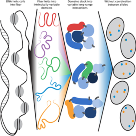
These methods have given considerable insights into genome organization at different length scales. The most basic unit of DNA organization is the chromatin fiber, formed by a DNA strand wrapping around histones. Different spacings and densities of histones create variable widths and conformations in the fiber. Super-resolution microscopy reveals the chromatin fiber to be made up of “clutches” or clusters of nucleosomes creating beads on a string along the DNA strand whose size corresponds to chromatin state: active chromatin with smaller clusters, inactive chromatin with larger clusters (Ricci et al., 2015). Cryo-electron microscopy has similarly revealed that DNA is found in a fiber between 5 and 24 nm in width with overall density depending on chromatin state (Ou et al., 2017). Furthermore, imaging approaches demonstrate that genome regions with similar chromatin states cluster within the nucleus (Boettiger et al., 2016; Smeets et al., 2014). These observations are consistent with the identification of compartments A and B defined in biochemical datasets and representing self-associating homotypic chromatin types which correlate well with their chromatin state as eu- or heterochromatin (Lieberman-Aiden et al., 2009).

Hi-C and related methods have led to the definition of self-associating domains on the order of hundreds of kb, referred to as topologically associating domains (TADs), which are highly reproducible features of Hi-C maps (Dixon et al., 2012; Nora et al., 2012; Sexton et al., 2012). TADs appear to be a fundamental unit of genome organization and to depend on the formation of loops mediated by the chromatin architectural proteins CTCF and cohesin (Mizuguchi et al., 2014; Nora et al., 2017; Sanborn et al., 2015; Gassler et al, 2017; Rao et al, 2017; Schwarzer et al, 2017; Wutz et al, 2017, Haarhuis et al., 2017). Visualization of individual TADs with super-resolution imaging reveals that they most often form discrete globules within the nucleus (Szabo et al., 2018). However, FISH and single cell Hi-C data have shown variability of interactions at the single cell level (Flyamer et al., 2017; Fudenberg and Imakaev, 2017; Giorgetti et al., 2014; Nora et al., 2012; Sanborn et al., 2015; Stevens et al., 2017; Ulianov et al., 2016). Furthermore, some evidence suggests TADs associate into higher-order structures (Fraser et al., 2015a; Moore et al., 2015; Weinreb and Raphael, 2015), but their precise arrangement is unknown (Benedetti et al., 2014; Darrow et al., 2016).

Biochemical interaction mapping methods provide a static view of genome conformation. In contrast, live-cell imaging studies have shown that individual loci undergo dynamic movement, consistent with constrained diffusion within a ~1.5 μm radius (Chubb et al., 2002; Fung et al., 1998; Lucas et al., 2014; Marshall et al., 1997). Furthermore, while most Hi-C methods are population-based and report the ensemble behavior of millions of cells, polymer-model based simulations and small scale studies to compare Hi-C datasets with imaging data point to extensive variability in genome organization between individual cells (Giorgetti et al., 2014; Kalhor et al., 2011; Tjong et al., 2016). Recently, single cell Hi-C experiments and super-resolution imaging have also illustrated variability in capture frequency (Carstens et al., 2016; Cattoni et al., 2017; Flyamer et al., 2017; Nagano et al., 2013; Ramani et al., 2017; Stevens et al., 2017; Tan et al., 2018). Thus, while it is increasingly obvious that the genome is flexibly organized, the nature and extent of variation in spatial genome architecture has not been examined systematically.

Here we have combined Hi-C and high-throughput imaging to map at a large scale the spatial position and colocalization frequencies of over a hundred pairs of genomic loci. We use this approach to comprehensively probe the heterogeneity of physical genome interactions and allele-specific behavior at the single cell level. Our findings reveal a remarkably high degree of cell-to-cell and allele-to-allele heterogeneity in spatial genome organization.

RESULTS

A combined Hi-C and hiFISH approach to systematically probe genome heterogeneity

To probe the patterns and extent of variation in spatial genome organization in a cell population, we applied hiFISH (high-throughput fluorescence in situ hybridization) (Shachar et al., 2015a) to systematically determine the spatial position and distances between combinations of large sets of genomic interaction pairs identified by Hi-C in human foreskin fibroblasts (HFFs). Hi-C maps were generated using four technical replicates of 25 million cells each and libraries were sequenced using 50 bp paired-end reads resulting in 746,195,659 mapped valid pairs. The Hi-C dataset was validated against a dilution Hi-C dataset of IMR90 cells (Jin et al, 2013), an in-situ Hi-C dataset of IMR90 cells (Rao et al, 2013), and an in-situ Hi-C dataset of HFF cells (Dekker et al., 2017). The relationship between contact frequency and genomic distance was very similar between the two dilution Hi-C datasets (Fig S1A) and all datasets showed significant overlap in TAD boundaries (Fig S1B), confirming that the HFF Hi-C dataset is comparable to others.

While the HFF Hi-C dataset allows resolution up to 10 kb, we chose to identify candidate interactions based on a 250 kb map to account for our use of Bacterial Artificial Chromosome (BAC) probes, which were used to increase labelling efficiency in high-throughput imaging and have an average size of ~200 kb. To create a comprehensive and unbiased probe set to explore the relationship of Hi-C interaction frequency and co-localization, we identified 125 probe pairs by screening the Hi-C data for 250 kb bins that had a large range in distance-matched Hi-C normalized read count at multiple distance thresholds (Fig. 1A, Tables S1, S2 for details on probe pairs). Our set included multiple associations with genome regions that were gene rich (6 or 10 genes within 250 kb) or gene poor (no genes within 250 kb) on chromosome 1, chromosome 17, and chromosome 18. This probe set maximizes the range of Hi-C frequencies (500-fold range), provides sets of distance-matched sites (similar genomic distances, up to 10-fold range in Hi-C frequency), enables probing of Hi-C-matched sites (similar Hi-C frequency, genomic distance ranging from 10 Mb to 250 Mb), and represents gene rich as well as gene poor regions (Fig 1A). In addition, two genome regions of 2.88 and 2.75 Mb, respectively, on chromosome 4, containing multiple TADs, were tiled at higher density (one probe at each TAD boundary and one probe centered inside each TAD, 25 BAC probes total) to examine short range associations (Fig 1A; Table S1). Since our intent was to probe general principles of association behavior and to avoid confounding effects, the functional status of the regions, such as transcriptional activity or epigenetic marks, was intentionally excluded from selection criteria. Nevertheless, ChIP-seq and RNA-seq data available from the ENCODE repository (ENCODE Project Consortium, 2012) for the closely related hTERT immortalized BJ skin fibroblasts indicated that regions in gene rich clusters generally showed increased mRNA expression, increased H3K4 and H3K36 methylation, and decreased H3K27 methylation as versus regions in gene poor clusters; two regions in gene poor clusters are outliers with high mRNA expression but were selected for low Hi-C interaction frequency with their respective baits (Table S1).

Figure 1: Spatial mapping of genome interactors.

A: Ideogram of loci used for spatial mapping. Orange bars: long-range sites. Blue bars: tiled regions. B: FISH image HFFs stained for three loci on chromosome 1. Blue arrows: spots separated by large distances. White arrow: all spots colocalized. Orange arrows: two of three spots colocalized. C: FISH image of an HFF stained for three loci on chromosome 4. D: Schematic diagram and Hi-C maps of “interactor” and “non-interactor”. E: 3D distance distributions minimal distances between “interactor” (brown) and “non-interactor” (blue). F-I: Distance distributions for distance-matched regions. 2D distances are used in panels H and I. J: Cumulative distance distributions for all tested pairs. Dashed line: median (50% total density). K-L: Coefficient of variation of spatial distance vs. Hi-C frequency or mean spatial distance for all 125 pairs.

The 125 interaction pairs were analyzed using a high-content screening approach to localize three regions per cell (Fig 1B, C) in ~500 cells per condition (see Methods). Distance measurements were not affected by chemical fixation and processing during the hiFISH procedure as demonstrated by comparable distance distributions between LacO and TetO portions of a previously described 25 kb LacO-TetO array in live cell imaging of NIH 2/4 mouse fibroblasts before and after fixation and permeabilization (Fig S2B, C) (Roukos et al., 2013) and consistent with prior observations that the FISH protocol does not disrupt DNA or RNA localization (Verschure et al., 1999). For all reported data, as previously observed, trends were similar using either 2D or 3D distances (Finn et al., 2017). 3D distances were used throughout to maximize accuracy.

Systematic comparison of interaction frequency to physical distance

We first sought to establish how Hi-C interaction frequencies relate to physical distances between interaction partners. We analyzed the distance distribution of a single bait probe on chromosome 1 and a “high-probability interactor” region 10 Mb upstream or an equidistant downstream “low probability interactor” region (Fig 1D, E). We observe a statistically significant difference in 3D spatial distance between these two targets with the upstream high-probability region at an average distance of 1.30 μm from the bait compared to 2.26 μm for the low-probability region (Fig 1E, p < 2.2*10⁻¹⁶). However, the distributions strongly overlap, with an overlapping coefficient of 0.57, indicating lack of clear separation at the single cell level. In fact, when analyzed on a single allele basis, 22% of bait spots were physically closer to the “low-probability interactor” than the “high-probability interactor” (Fig 1E). An even larger overlap was observed for 4 additional distance-matched pairs at various distances from 400 kb to 20 Mb separation and with 2–5 fold differences in Hi-C capture frequency (Fig 1F–I).

To expand this analysis, we determined cumulative distributions of pairwise spatial distances for the entire set of 125 interaction pairs (Fig 1J). The median spatial distances of pairs strongly correlated with their Hi-C frequencies (Fig 1J, Fig S4C). However, the distance distributions lacked multimodality or discontinuity (Fig 1J), suggesting that the overall population of distances is variable and continuous, consistent with findings from single cell Hi-C or imaging of select loci (Giorgetti et al., 2014; Nagano et al., 2013). Analysis of noise in the association frequencies at all 125 locus pairs via the coefficient of variation shows that regions with high Hi-C contact frequencies and moderate-to-small mean spatial distances tend to have the greatest spread of coefficient of variation in distances (Fig 1K, L). Overall, these observations point to extensive heterogeneity in physical proximity of Hi-C interaction pairs in individual cells.

The steady-state association frequencies of genomic interactors are low

To provide a more direct comparison with Hi-C interaction frequency, we measured frequency of perfect colocalization (defined as coincident local intensity maxima between two FISH signals) for 106 interaction pairs with a range of Hi-C frequencies over two orders of magnitude (1.8*10⁻⁴ to 6.2*10⁻²; Fig 2A, Fig S3). We found good correlation between Hi-C frequency and colocalization (Fig 2B; r² = 0.861, p < 2.2*10⁻¹⁶) with colocalization in between 0.04% and 27.3% of alleles (Fig. 2B). For most pairs (102/106) less than 10% of alleles in the cell population colocalized, and only one pair showed colocalization at more than 15% of alleles in the population, although the dataset included many pairs within the top 20% of Hi-C capture frequencies. To eliminate potential confounding effects due to limited imaging resolution or possible systematic drift between imaging channels, the distance threshold was relaxed to 350 nm, the distance at which 95% of co-stained loci are reliably colocalized (Roukos et al., 2013). At the same time, this approach captures potential colocalizations within a chromatin microcompartment (Szabo et al., 2018). We find the same strong correlations between Hi-C frequency and spatial proximity at this relaxed threshold (Fig 2C, r² = 0.903, p < 2.2*10⁻¹⁶) with colocalization frequencies from 0.26% to 53.66%. 89/106 interaction pairs showed colocalization in fewer than 30% of alleles and only a few interaction pairs (3/106) showed colocalization in more than 50% of alleles (Fig 2C). Similar trends were observed upon using distance thresholds of 200 nm or 1 μm or when considering mean 3D distances (Fig S4).

Figure 2: Correlation between Hi-C, genomic distance, and colocalization.

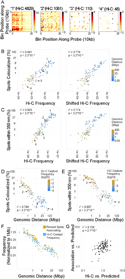
A: 10 kb resolution Hi-C maps of 250×250 kb regions centered on four interactions with variable Hi-C frequencies. These pairs are marked as 1–4 in subsequent scatter plots. B, C: Scatter plot of percentage of spot pairs with measured 3D distance = 0 (B) or < 350nm (C) vs. Hi-C frequency or shifted Hi-C frequency. D, E: Scatter plot of percentage of spot pairs with measured 3D distance = 0 (D) or < 350nm (E) vs. genomic distance. F: Scatterplot of enrichment of percent spots associating or Hi-C capture frequency vs. 1 Mb average for each site pair vs. genomic distance. G: Scatterplot of values normalized by distance-based predictions. Predicted values were generated based on a single power law model, and the ratio between predicted and observed value was used.

Analysis of root mean squared error (RMSE) using a power-law model indicated an overall spread of ~2.6-fold from the model, consistent with a ~2.6-fold range in colocalization percentage between pairs with similar Hi-C frequencies, indicative of heterogeneity between associations. These results demonstrate a low overall frequency of colocalization in the population, and a remarkably high degree of variability in association frequencies and spatial separation of genome regions in individual cells across a population.

Genomic distance as a key determinant of association frequencies

As a control for the above analysis, we calculated Hi-C frequencies for pairs with both bait and target shifted downstream by 500 kb. This approach maintains the genomic distance for each pair while removing sequence-specific effects. We find slightly decreased correlation between Hi-C frequency and colocalization for shifted regions at all distance thresholds (Fig 2B, r²: 0.776 for perfect colocalization, r²: 0.774 for 350 nm threshold), suggesting a considerable contribution of genomic distance to contact probability. To further explore the contribution of genomic distance to association frequencies, we correlated association frequencies for all 125 interaction pairs with their genomic distance (Fig. 2D–E). We find a strong inverse correlation between association frequency and genomic distance both for perfect colocalization (Fig 2D; r²: 0.786, p < 2.2*10⁻¹⁶) and for colocalization within 350 nm (Fig 2E; r²: 0.907, p < 2.2*10⁻¹⁶). As observed for Hi-C frequencies, RMSE analysis indicated a 2–3 fold variation in percent colocalization for locus pairs at similar genomic distances; for example, two locus pairs separated by very similar genomic distances (412 and 419 kb) colocalized with significantly different frequencies of 46% and 26% of alleles, respectively (Fig 2D, E). We also find very similar distance-related decay between the percentage of spots within 350 nm and Hi-C capture frequency (Fig 2F), suggesting a major contribution of genomic distance to interaction frequency.

To determine whether genomic distance is sufficient to explain the correlation between Hi-C capture frequency and association frequency, for each of the 106 probe pairs we calculated the expected Hi-C frequency and percent colocalization based on genomic distance alone and determined fold-changes from this expected value. We find that a weak correlation between HiC and colocalization frequencies is maintained (r² = 0.138, p = 2.1*10⁻⁵, Fig 2G). These findings suggest that the observed correlation between Hi-C frequency and colocalization can largely be explained by genomic distance and that structural features of the chromatin fiber, such as loops and TADs, act primarily as modulators of physical associations driven by sequence proximity.

Gene density and chromatin properties modulate interaction frequencies

To investigate whether chromatin context affects the likelihood of spatial proximity, 46 loci on chromosomes 1, 17, and 18 were classified into four clusters based on chromosome and gene density (see Methods; Table S1). Locus pairs between gene rich regions (1–11 genes, median 4) showed greater heterogeneity between distance-matched regions and overall weaker correlation with genomic distance than loci in gene poor regions (0–5 genes, median 2) (Fig 3A). Gene rich loci also exhibited a wider range of association frequencies than gene poor regions (Fig 3B). These observations demonstrate greater distance dependence and smaller variation of physical association between locus pairs in gene poor regions of the genome than those in gene rich regions. This is consistent with a model in which gene-poor chromatin is characterized by broad chromatin compaction and gene-rich chromatin is more dispersed, but undergoes specific interactions such as locus-specific loops (Boettiger et al., 2016; Lieberman-Aiden et al., 2009).

Figure 3: Modifiers of association frequencies.

A: Scatterplots of percentage of spot pairs within 350 nm vs. genomic distance. Line of best fit indicated. B: Violin plots of percentage of spot pairs within 350 nm. C: Violin plots of percentage of spot pairs within 350 nm by compartment. D: Scatterplot of percentage of spot pairs within 350 nm vs. genomic distance. E: Scatterplot of association likelihood vs. Hi-C score, normalized to a distance-based power law model.

We next probed for differences in association frequencies of loci in compartments A or B as defined by Hi-C (Boettiger et al., 2016; Lieberman-Aiden et al, 2009; Smeets et al., 2014). While the probe set selected was somewhat under-represented for probes pairs in which both probes were in the A compartment, associations between loci occur nonetheless with slightly higher frequency among pairs where both loci belong to compartment B than A-A or A-B pairs (Fig 3C). This behavior is especially evident when considering power-law models of associations sorted by compartment (Fig 3D) and is consistent with observations of Hi-C frequencies, where pairs within the B compartment tend to have higher Hi-C capture frequencies than the genome-wide distance-based power law model (Fig 3E). These observations are in line with a model of A and B compartments representing distinct sets of interactors, and with the notion that B compartments are more compact and self-associating at these distances, while A compartments are more dispersed and variable in their interactions (Boettiger et al., 2016; Lieberman-Aiden et al., 2009; Sexton et al., 2012).

Variability in intra- and inter-TAD interactions

TADs are regions of the genome defined by elevated Hi-C interaction frequencies for locus pairs within the region as compared to locus pairs at similar distances outside the region (Dixon et al., 2012; Nora et al., 2012). We determined the variability in interactions within and between TADs by high-throughput single cell imaging using BAC probes for coarse mapping and 10 kb probes for fine mapping of interactions (Fig 4).

Figure 4: Enrichment of Intra-TAD interactions.

A-C: Hi-C plots showing regions tiled with location of probes marked (black bars) and TADs color-coded. D: FISH image using 10 kb probes and positive control BAC. E: Hi-C snapshots and distance distributions for distance matched interaction pairs between and within TADs, as measured by BAC probes. F: As in E, but with 10 kb probes. Non-significant p-value marked in red. G: Box plots showing distribution of percent spots within 150 or 350 nm. Boxes: BAC probes, points: 10 kb probes.

To validate the use of BAC probes, which are approximately 200 kb in size and as such on the same size scale as a typical TAD, we determined baseline levels of separation due to optical drift and aberrations by imaging a single probe stained in all three colors and compared this positive control for 100% interaction to pairs of probes that were either overlapping, adjacent, or proximal (Fig S5). We found that as long as the probes did not overlap by more than 50%, they showed noticeably fewer colocalization events than co-stained loci, suggesting that BAC probes are able to accurately measure colocalization at this length scale (Fig S5). It is worth noting that our measurements erred toward over-estimating the colocalization of any two smaller regions, since tight colocalization at any part of the BAC probe would tether the two probes together and likely be scored as a colocalization event.

To probe the variability of spatial organization of individual TADs in single cells in a population, we selected two regions on chromosome 4 encompassing a total of 14 TADs, identified in Hi-C datasets binned at 20 kb, and measured distances at 15 locus pairs within the same TAD at varying distances (from 70 kb to 600 kb) and across an 8-fold range of Hi-C frequencies (Fig 4A, B) as well as 56 locus pairs separated by at least one TAD boundary (from 240 kb to 2.7 Mb genomic distance). For higher resolution measurements, we cloned 10 kb probes specifically targeting TAD boundaries or internal regions in a 2 Mb sub-portion of the region probed by BACs and encompassing three TADs (Fig 4C, 4F). For increased spatial resolution, probes were imaged using deconvolution microscopy, and spot centers were determined at sub-pixel resolution by calculating a center of gravity (Fig 4D).

Examination of individual distance-matched interaction pairs by cumulative distribution functions (ECDF) confirmed enrichment for interactions within a TAD as compared to interactions between two TADs, both with BAC probes and with 10 kb probes (Fig 4 E, F; p-values < 10⁻⁴ KS-test). We observed a maximum of 5-fold enrichment in percent colocalizing at 150 nm (Fig 4F; 500 kb, 0.70% between TADs vs 3.36% within the TAD) and a maximum of 3-fold enrichment at 350 nm (Fig 4F; 300 kb #2, 21.82% vs 64.74%). These observations were confirmed and generalized by analysis of all BAC and 10 kb probe pairs separated by between 240 and 570 kb, representing a set of roughly distance-matched probes (Table S2; Fig S5C). We find a statistically significant 1.5–2 fold enrichment for colocalizations within a TAD as compared to those between two TADs when considering only BAC probe data (Fig 4G; 150 nm: p = 0.003702, 350 nm: p = 0.0274, Wilcoxon) or BAC and 10 kb data combined (Fig 4G; 150 nm: p = 0.01352, 350 nm: p = 5.869*10⁻⁴, Wilcoxon). We conclude that interactions within a single TAD are modestly enriched as compared to interactions between TADs at a similar distance, but high-frequency interactions remain relatively rare.

Higher order organization of TADs

We next sought to investigate the higher order organization of multiple TADs (Fraser et al., 2015a; Moore et al., 2015; Szabo et al., 2018; Wang et al., 2016; Weinreb and Raphael, 2015) by probing interactions between boundaries, intra-TAD interactions, and interactions between an internal probe and a boundary probe (Fig. 5A). Five boundary pairs, 17 internal pairs, 25 mixed pairs, and 15 pairs within individual TADs were considered for a total of 62 pairs (Fig. 5B). Scatterplots comparing the percent of colocalization relative to genomic distance showed that intra-TAD, internal, boundary, and mixed interaction pairs all form overlapping distributions (Fig 5B). While a power-law model revealed that boundary pairs were the most distance dependent, followed by mixed pairs and internal pairs, all types of locus pairs outside of TADs showed similar scaling with respect to Hi-C frequency (Fig 5B). Considering only regions separated by at least 750 kb or fitting an exponential rather than a power-law to the data did not significantly change the trends or r² values. These differences in scaling suggest that internal regions of adjacent TADs, rather than TAD boundaries, are most likely to interact.

Figure 5: Neighboring and nearby TADs associate at internal regions, not boundaries.

A: Diagram of four classes of interactions. B: Scatterplots of percentage of spot pairs within 350 nm (top panels) or 150 nm (bottom panels) vs. either genomic distance (left panels) or Hi-C capture frequency (right panels). C: CDFs of 3D distances for boundary element association and internal region association using 10 kb probes. Non-significant p-value in red. D: Representative image of tight colocalization of BAC probe and two 10 kb probes. E: Barplot of proportion of triplet clusters (colocalization of all three probes) vs. expected numbers based on an assumption of statistical independence between pairwise interactions. Triplet IDs in Table S3. F: CDFs of distance distributions for upstream 10kb probes, classified based on distance from BAC to downstream 10kb probe. Downstream probe farther than median: light blue. Downstream probe is closer than median: dark blue. Maps at the right show location of probe pairs tested. Non-significant p-values in red. G: Scatterplots showing lack of correlation between distance to upstream and downstream 10kb probes.

To eliminate the possibility that these observations were confounded by the size of the BAC probes used, we examined three pairs of TAD boundaries, separated by 500 kb, 900 kb, or 1.1 Mb, using 10 kb probes placed precisely at the TAD boundaries or fully within the TADs (Fig 5C). No increase in the proximity of boundary elements compared to internal regions at the same genomic distance was found (Fig 5C). On the contrary, internal regions had a modest tendency to be closer together than boundary elements (Fig 5C). These results demonstrate that TAD boundaries do not consistently interact more frequently than internal regions.

Despite these observations, multiple TAD boundaries may still be brought together into higher-order interactions either due to coregulation or mutual stabilization (Beagrie et al., 2017; Darrow et al., 2016; Olivares-Chauvet et al., 2016). To directly test this model, we measured colocalization rates of three or more boundary elements amongst neighboring TADs. While we do observe instances where all three probes are within 350 nm (Fig 5D), internal regions form triplets at similar rates to boundary regions, suggesting that boundary regions are not unique in their ability to form higher order structures (Fig 5E). Importantly, we do not find evidence of stabilization or coregulation since the observed association frequencies are in line with those predicted based on simple pairwise association frequencies and an assumption of statistical independence (Fig 5E). These results were confirmed using 10kb probes (Fig 5F,G). Taken together, these observations suggest that although boundaries form the edges of internally interacting TADs, and while most of the TADs examined do show evidence of corner peaks in high-resolution Hi-C data (Fig S5), these loops do not necessarily co-occur or bring the boundaries of neighboring TADs together more frequently than adjacent internal regions. Furthermore, neighboring TAD boundaries do not appear to cluster, consistent with a model where loops are independent events likely dynamically formed and sporadically dissolved (Fudenberg et al., 2016; Sanborn et al., 2015).

Independent behavior of individual alleles creates intrinsic variation in spatial genome organization

Our observations demonstrate considerable variance in spatial distance between any two loci at the single cell level, regardless of their likelihood of interaction. This variability may represent heterogeneity in the behavior of alleles in individual cells, or it may be the result of cell-to-cell variation while the behavior of alleles in the same cell is coordinated. To distinguish between these possibilities, we probed the behavior of the two alleles in individual cell nuclei for all 125 comparisons by measuring the minimal distances of each allele relative to their interaction partners in single nuclei (Fig 6A; Fig S6A). Scatter plots demonstrate little correlation between the behavior of the two alleles in a given nucleus for any of the interaction pairs (Fig 6A; Fig S6A). When individual nuclei were categorized based on how many colocalization events they contained, the vast majority of cells (70.04–99.46%) contained no events, a limited fraction (0.54–24.24%) contained one event, and very few (0.02–5.34%) contained two events (Fig 6B, Fig S6B), which is in line with the observed low prevalence of overall interactions in the population. In no case did more than 6% of cells contain two simultaneous interactions (Fig 6B; Fig S6B). These data reinforce the observed low prevalence of colocalization throughout the population and demonstrate that interactions most frequently occur independently at the two homologous chromosomes within a nucleus.

Figure 6: Allelic independence of interactions.

A: Scatterplots of minimal distances of both alleles of an interaction pair on a per-cell basis at the most correlated site pair, least correlated site pair, and most anti-correlated site pair. B: Bar graph showing observed and expected proportion of cells with 0, 1, or 2 associations within 350 nm between spots for a variety of selected site pairs. C: Scatterplots showing correlation of distances between bait and two targets (upstream target and downstream target) on a per-bait basis, for most correlated, most anti-correlated, and least correlated triplets. D: Bar graph showing observed and expected proportion of bait spots with a triplet association within 350 nm for selected triplets. E: Bar graph showing observed and expected proportion of cells with 0, 1, or 2 triplet associations for selected triplets. For all comparisons, see Figure S6. Probe IDs for all panels in Table S3.

In addition to pairwise associations, it has been suggested that multiple gene loci may physically form clusters, possibly due to mutual stabilization of pairwise interactions or chromatin context (Beagrie et al., 2017; Olivares-Chauvet et al., 2016). To assess the extent and cell-to-cell variability of clustering of multiple interaction pairs, we measured the degree of covariation between multiple site pairs on the same chromosome and generated scatter plots of the spatial distance from a single bait to an upstream target vs. the distance from the same bait to a downstream target (Fig 6C, S6C). No evidence of clustering of multiple pairs was found, with a maximum r² = 0.1311 for all combinations (Fig 6C; Fig S6C). Enrichment over expected values as calculated from pairwise association frequencies was detected sporadically (probes 375/354/422 and 11/52/91). However, cluster formation was rare, occurring at less than 15% of loci for even the most prevalent clusters. These results were confirmed by direct counting of clusters in individual cells with 66–99% containing no triplet clusters, less than 30% containing one cluster, and less than 5% containing two clusters (Fig 6E, Fig S6E). Our observations indicate that non-specific clustering of multiple interaction pairs is not a general principle of higher order genome organization, and that reported clustering of genes with complex regulatory hubs (Ay et al., 2015; Beagrie et al., 2017; Ferraiuolo et al., 2010; Morey et al., 2007) may be a locus-specific rather than general effect, or may reflect their tendency to interact as seen in population-averaged data rather than a requirement for formation of such hubs in individual cells.

DISCUSSION

We demonstrate a remarkably high level of heterogeneity in spatial genome organization among individual cells and between alleles in the same cell. Our conclusions are based on analysis of Hi-C datasets by systematic high-throughput imaging to determine the variability of genome architecture in a population at the level of single cells and alleles. This approach takes advantage of the genome-wide nature of Hi-C datasets and the ability of high-throughput imaging to probe genome organization at the single cell level with high statistical power by imaging an extensive set of locus pairs in a large number of individual cells. Our method overcomes the limitations of traditional biochemical mapping methods which generate population averaged datasets and at the same time elevates traditional imaging methods beyond their anecdotal nature due to small sample sizes.

We find a high level of variability in how the genome folds in individual cells. In our analysis, long range associations (> 5 Mb) typically occur in no more than 10% of alleles for any locus pair, while a small number of such distal associations are present in 20–25% of cells. The relatively low frequency of mid- and long-range associations in the population and the combinatorial occurrence of multiple associations in individual cells suggest that a wide spectrum of genome-wide organizational patterns exist in a cell population (Giorgetti et al., 2014; Kalhor et al., 2011). Some of the variability observed in long-range interactions may be a reflection of dynamic cycles of association and dissociation in living cells such as those seen over short distances in promoter-enhancer interactions (Chen et al., 2018). However, dynamic motion cannot explain all observed variation, since even the most common long-range interactors mapped here are often found at significantly larger distances than those observed for intrinsic dynamic motion, which are typically constrained within 1.5 μm (Chubb et al., 2002; Fung et al., 1998; Marshall et al., 1997).

We find that genomic distance is a major determinant of physical association of genomic loci. In fact, most of the observed correlation between FISH colocalization and Hi-C frequency can be accounted for by the effect of genomic distance, with proximal loci more frequently interacting. This interpretation is consistent with a model of DNA organization in which the chromatin fiber is not consistently arranged in 3D space and thus exhibits a large variability from cell to cell as observed here and in single cell Hi-C analyses (Flyamer et al., 2017; Fudenberg and Imakaev, 2017; Giorgetti et al., 2014; Nora et al., 2012; Sanborn et al., 2015; Stevens et al., 2017; Szabo et al., 2018; Ulianov et al., 2016). However, our comparative analysis demonstrates that genomic distance alone is not sufficient to explain all interaction patterns. In particular, gene dense regions tend to show more heterogeneity in interaction frequencies between locus pairs. Furthermore, we find that at the distances studied, loci in the A compartment are overall less likely to interact than those in the B compartment, consistent with Hi-C analyses which have shown distinct organization patterns in different compartments (Boettiger et al., 2016; Francis et al., 2004; Lieberman-Aiden et al., 2009; Wang et al., 2016). Both of these observations are consistent with a model in which repetitive, non-genic sequences, often located at the center of a chromosome territory, sample a smaller total volume than genes (Hall et al., 2014). Our findings suggest that overall genome organization at large genomic distances is highly variable and likely to be modulated by a combination of genomic distance, chromatin state, and gene content.

While we observe that loci within a TAD colocalize at relatively high frequencies, we also find that loci in adjacent TADs interact robustly and are only reduced two- to three-fold. Our findings that interactions between regions in the same TAD are not necessarily pervasive and that interactions are also common between neighboring TADs are in line with single cell Hi-C and super-resolution imaging studies which demonstrated that while TADs often form contiguous globules or microcompartments, individual cells exhibit widely distinct TAD structures (Carstens et al., 2016; Cattoni et al., 2017; Flyamer et al., 2017; Giorgetti et al., 2014; Nagano et al., 2013; Stevens et al., 2017; Szabo et al., 2018). We also observe a preference for inter-TAD associations between internal regions in distal TADs, rather than TAD boundaries, consistent with a model in which the loops that form TADs are dynamic and mobile structures (Fudenberg et al., 2016; Hansen et al., 2018). In line with this interpretation, we find no evidence for clustering of boundaries.

Variability in association frequencies may either be due to extrinsic causes such as signaling or stable subpopulations of cells or may be cell-intrinsic (Fu and Pachter, 2016). Our observation of independence between the two alleles in the same cell provides strong evidence for primarily cell-intrinsic patterns of variation: most of the observed variability is intrinsic to individual chromosomes. Furthermore, the existence in our dataset of cells in S or G2, observed as closely clustered doublets in all channels, suggests that this intrinsic variability may be present throughout the cell cycle. Similarly, our finding that two interactions on the same chromosome occur independently is inconsistent with widespread co-regulation or cluster formation. It is possible that in intact tissues, or at different loci, extrinsic variability plays a larger role. However, these data suggest high basal levels of intrinsic variability in pairwise interactions.

Our data provide direct experimental support for conclusions from early predictive computational models based on tethered conformation capture (TCC) which suggested that interaction maps are the composite of multiple genome configurations and that the patterns of individual interactions differ between cells (Giorgetti et al., 2014; Kalhor et al., 2011). Our analysis of thousands of individual cells is also in line with studies on transcriptional bursting which suggest that even promoter-enhancer loops and association with the transcriptional machinery may show notable variability between cells and, over time, in a single cell (Chen et al., 2018; Coulon et al., 2013; Lim et al., 2018). These observations suggest a model in which dynamic and variable chromatin structures, interacting with dynamic and variable protein complexes, act in concert to provide a stable transcriptional response across a population, or in single cells over time. A key question to be addressed in future work is how functional stability arises in the context of this heterogeneous genomic landscape to ensure execution of gene expression programs in response to physiological stimuli. This study provides a foundation for such work by characterizing in a systematic and quantitative fashion the extent and nature of the heterogeneity and variability in higher order genome architecture. Our results support a view of genome organization as plastic, heterogeneous, and marked by variability between individual cells and alleles.

STAR Methods

CONTACT FOR REAGENT AND RESOURCE SHARING

Further information and requests for resources and reagents should be directed to and will be fulfilled by the Lead Contact, Tom Misteli (mistelit@mail.nih.gov).

EXPERIMENTAL MODEL AND SUBJECT DETAILS

Cell Lines

Male human foreskin fibroblasts (HFF) immortalized with hTert via neomycin selection as described previously (Benanti and Galloway, 2004) were grown in DMEM with 10% FBS, 2 mM glutamine, and penicillin/streptomycin and split 1:4 twice weekly. These cells are the parental HFF line to the HFFc6 common cell line used in the 4D Nucleome. Their karyotype was verified as normal via SKY staining (data not shown). HFFs between passages 40 and 45 were plated at a density between 5000 and 7500 cells per well in 384 well plates (CellCarrier or CellCarrier Ultra, PerkinElmer), and left to grow and settle overnight before fixation in 4% paraformaldehyde for 20 minutes. After fixation, plates were rinsed twice in PBS and stored in 70% ethanol at 20°C for up to two months. A total of 40 hiFISH exp eriments were performed in 42 wells and 14 probe combinations (3 wells per probe combination) per experiment. 500–1000 cells were imaged per probe combination per experiment, for a total of 615,414 spot pairs used in high throughput analysis.

METHOD DETAILS

High-throughput Chromosome Conformation Capture

Hi-C libraries were generated from HFF cells cross-linked in 1% formaldehyde as described previously (Lieberman-Aiden et al., 2009; Naumova et al., 2013; Nora et al., 2012). Four technical replicates of 25 million cells each were generated. The libraries were sequenced using 50 bp paired-end reads with a HiSeq2000 machine with each replicate in its own lane and replicates 3 and 4 sequenced two more times in one lane. The eight lanes were pooled; the total number of valid pairs after mapping and filtering was 746,195,659. The filtered reads were mapped to the human genome (hg19) using Bowtie 2.2.8 and normalized using the iterative mapping strategy described previously (Imakaev et al., 2012; Lajoie et al., 2015).

Probe selection

For long-range interactions within chromosomes (> 10 Mb separation), Hi-C data was binned at 250 kb and associations classified into proximal (separated by ~ 10 Mb or 10% of the chromosome), medial (separated by ~ 50 Mb or 30% of the chromosome), and distal (separated by ~ 100 Mb or 50% of the chromosome) and subsequently ranked into likely interactors (top 100 interactions based on Hi-C signal at a given distance), unlikely interactors (bottom 100 interactions at a given distance), or median (median 100 interactions at a given distance). Probe families were selected as those with a single bait and representative targets from as many categories (e.g. proximal, likely interactors vs. distal, likely interactors) as possible. Probe families were further classified as either gene rich or gene poor based on gene content of the central bait probe: gene rich families were selected for those with more than five genes overlapping the central bait probes, gene poor families had no genes overlapping the central bait probe. Finally, each probe was assigned a compartment, calculated from the first principle component of the normalized Hi-C data. For short range interactions (< 3 Mb separation), two regions on chromosome 4 were chosen by visual inspection to contain several adjacent TADs likely within the same compartment. These regions were tiled using adjacent/overlapping BAC probes, using, if possible, probes to position a BAC probe at the base/boundary between each TAD-like structure and one within each TAD-like structure. For TADs that were too small for tiling without substantial overlap between adjacent BAC probes, only boundary or only interior probes were chosen. A table of the start and end locations of all BACs used is included as Table S1.

In all cases, pairwise Hi-C frequencies, bias scores, and z-scores were calculated on the basis of a 250 kb bin centered around the BAC probe used. Pairs within the top 5% of bias scores or with z-scores with an absolute value above two were considered low-quality Hi-C frequencies and excluded from further analyses involving Hi-C frequency. A table of all pairwise associations tested, along with Hi-C scores calculated for the centered 250 kb bin, bias scores, and percent spots associating is included as Table S2.

For 10 kb probes, 10 kb regions of interest were selected based on Hi-C data and TAD structure within one of the regions tested on chromosome 4 (chr4:55000000–57000000). Four adjacent TAD boundaries were targeted, and the intervening TADs were tiled with one probe every 100 kb. Primers were identified to amplify each 10 kb region in three chunks, and the regions were cloned from genomic DNA. Nick translation was performed on mixed pools of two or three plasmids. A complete list of probes is provided in Table S1.

Segmenting Hi-C data into domains

We segmented Hi-C data de novo to compare TAD boundaries between HFF and IMR90 cell lines, and dilution Hi-C versus in situ Hi-C. Segmentation was done on data binned at 10 kb resolution with the lavaburst software package described previously (Schwarzer et al., 2017). As input to the segmentation model, we used the corner score algorithm with default parameters, and Hi-C matrices where columns and rows with fewer than 100 total reads were masked out. Segmentation was performed for a single chromosome at a time. Only domain boundaries larger than 40 kb were kept for downstream analyses.

The percentage of overlap between called domain boundaries in two different data sets was computed: first, domain boundary start and end pairs were flattened into a single list and filtered for unique boundary locations. This procedure was repeated for each experimental condition and each chromosome separately. As a normalization factor for the percentage overlap between conditions, we obtained the total number of identified boundaries and kept the smallest of the two values. The overlap between domains was computed by pair-wise distances between unique boundary locations. Boundaries were considered overlapping if their distance was less than or equal to 10 kb. The total count of overlapping boundaries was then divided by the total number of identified boundaries (as described above) to yield the overlap percentage. The computation was performed for each chromosome, and these were considered independent measurements of overlap for the purposes of statistical testing (see below).

As a control/baseline for boundary overlap, we shifted all domain boundary locations by 100 kb for one of the two data sets being compared and repeated the overlap calculation. This procedure controlled for the basal level of association due to random chance, while ensuring that the sizes and relative locations of domains were maintained. The non-parametric Mann-Whitney U test was used to score statistical significance overlap percentages obtained for the shifted and unshifted boundaries.

Binning Hi-C data to obtain Hi-C scores

To convert high resolution data (e.g. binned at 10 kb) to lower-resolution data (e.g. binned at 250 kb), we performed the following: First, for any desired 250 kb window composed of a 25 by 25 grid of 10 kb bins, we summed the normalized 10 kb resolution Hi-C data over all the bins and divided by 25. The normalization by 25 (instead of dividing by 25 squared = 625) is explained as follows: First, consider that summation is over normalized data. We can break down the procedure of summing of the 25 by 25 window as summing over columns first, then summing over rows. We note that the ICE normalization procedure results in columns (and rows) of the Hi-C matrix that that separately sum to 1. As such, following ICE normalization, each bin along any column of the Hi-C map at 10 kb resolution will have approximately 1/25th of the value (contact frequency) of an equivalent bin in a 250 kb map since there are 25-fold more bins and the total Hi-C contact frequency is subdivided between these bins. Since bins in normalized 10 kb binned data are already divided by 25, we only need to divide by a further 25 to account for the fact that there are 625 additional bins in the 25 by 25 window. To obtain Hi-C scores for windows centered on the 10 kb FISH probe locations, we did the same procedure above, but coarse grained from 1 kb binned Hi-C data to 10 kb. The conversion factor in this case was a factor of 10 (instead of 25).

HiFISH Imaging

High-throughput fluorescence in-situ hybridization (hiFISH) was performed as described previously (Burman et al., 2015; Finn et al., 2017; Shachar et al., 2015b). Probes were generated by a nick translation reaction incubated at 14°C for 1 hr 20 min with the following mix: 40 ng/μL DNA, 0.05 M Tris-HCl pH 8.0, 5 mM MgCl2, 0.05 mg/mL BSA, 0.05 mM dNTPs, including fluorescently tagged dUTP, 1 mM β-mercaptoethanol, 0.5 U/μL E. coli DNA Polymerase and 0.5 μg/μL DNAse I. The reaction was stopped with the addition of 1 μL EDTA per 50 μL reaction volume and heat shocked to 72°C for 10 m in, then stored at −20°C overnight. QC gels were run in 2% Agarose to verify successful nick translation with a smear of less than 1 kb. Combinations of three probes (1 μg per probe) were mixed, ethanol precipitated, resuspended in 15 μL of hybridization buffer (50% formamide pH 7.0, 10% Dextran Sulfate, and 1% Tween-20 in 2X SSC) per well and warmed to 72°C before plating.

Cells were removed from ethanol and rinsed twice in PBS before permeabilization. Cells were permeabilized in 0.5% w/v saponin/0.5% v/v triton X-100 in PBS at room temperature for 20 minutes, rinsed twice with PBS, deproteinated for 15 minutes at room temperature in 0.1 N HCl, and neutralized for 5 minutes at room temperature in 2X SSC before equilibration in 50% formamide/2X SSC for at least 30 minutes at room temperature. 13 μL of resuspended probe mix was added per well, pipetting to mix just before adding, and plates were spun to remove bubbles. Cells were denatured for 7.5 minutes at 85°C and immediately moved to a 37°C water bath for 72 hr hybridization. After hybridization, plates were rinsed once at room temperature with 2X SSC, and then thrice each with 1X SSC and 0.1X SSC both warmed to 45°C. Cells were stained with DAPI (3 μg/mL) for 15 minutes, rinsed, mounted in PBS, and imaged. All experiments were performed in triplicate.

Imaging on chromosomes 1, 17, and 18 was performed in four channels (405, 488, 561, 640 nm excitation lasers) in an automated fashion using a dual spinning disk high-throughput confocal microscope (PerkinElmer Opera QEHS) with a 40X water immersion lens (NA = 0.9) and pixel binning of 2 (pixel size = 320 nm). 20–40 fields of view were imaged per well. In all exposures the light path included a primary excitation dichroic (405/488/561/640 nm), a 1^st emission dichroic longpass mirror: 650/660–780, HR 400–640 nm and a secondary emission dichroic shortpass mirror: 568/HT 400–550, HR 620–790 nm. In exposure 1, samples were excited with the 405 and 640 nm lasers, and the emitted signal was detected by two separate 1.3 Mp CCD cameras (Detection filters: bandpass 450/50 nm and 690/70 nm, respectively). In exposure 2, samples were excited with the 488 nm laser and the emitted signal was detected through a 1.3 Mp CCD camera (Detection filter: bandpass 520/35). In exposure 3, samples were excited with the 561 nm laser and the emitted light was detected through a 1.3 Mp CCD camera (Detection filter: bandpass 600/40). Samples were optically sectioned in z every 1 μm for a final volume of 7 μm. For clustering experiments, samples were optically sectioned in z every 300 nm for a final volume of 7 μm.

For short range interactions on chromosome 4, imaging was performed in four channels (405, 488, 561, and 640 nm excitation lasers) in an automated fashion using a dual spinning disk high-throughput confocal microscope (Yokogawa CV7000), using a 60x water immersion lens (NA = 1.2) and no pixel binning (pixel size = 108 nm). 16 fields of view were imaged per well. In exposure 1, samples were excited with the 405 and 561 nm lasers, and the emitted light was collected through a path including a short pass emission dichroic mirror (568 nm) and two sCMOS cameras (5.5 Mp) in front of 445/45 nm and 600/37 nm bandpass emission filters, respectively. In exposure 2, samples were excited with the 488 and 640 nm lasers, and the emitted light was collected through the same light path and with the same cameras as exposure 1, but with 525/50 nm and 676/29 nm bandpass emission filters, respectively, instead. Samples were optically sectioned in z every 1 μm for a final volume of 7 μm.

Since HFFs are diploid, experiments in which we detected exactly two FISH signals per locus in fewer than 60% of cells were excluded and only cells which showed the same number of spots in each channel, and at least two spots in each channel, were considered in the analysis. In the final analysis, all reported data were generated from sets of at least 500 FISH signal pairs, with an average of 4,365 spot-spot distances analyzed per probe pair.

To identify pairs on the same chromosome, we identified minimum distances between FISH signals of different colors on a per-green-spot basis (for green:red and green:far red comparisons) or a per-red-spot basis (for red:far red comparisons). The distribution of minimum distances between loci showed little overlap with the distribution of maximum distances (Fig S2A), demonstrating that hiFISH accurately distinguishes multiple loci on the same chromosome from those on homologous chromosomes (Finn et al., 2017).

FISH and Deconvolution Imaging of 10 kb probes

FISH was performed on slides using the same protocol as plates with the following alterations: 10 kb probes were used at a concentration of 200 ng per 15 μL hybridization mix, and BAC probes at a concentration of 2 μg per 15 μL hybridization mix. Coverslips were sealed with rubber cement before denaturation at 85°C. After primary washes, coverslips were washed for 10 minutes in 0.05% tween-20/4X SSC at room temperature and blocked in 3% BSA/0.05% tween-20/4X SSC for 20 minutes at 37°C. Avidin-FITC was diluted 1:400 in block solution, Avidin-Cy5 was diluted 1:2000 in block solution, and α-Digoxygenin-TRITC was diluted 1:400 in block solution. Coverslips were incubated in antibody solution for 45 minutes at 37°C in a humid chamber, washed four times in 0.05% tween-20/4X SSC at 45°C, and washed four times in PBS at room temperature. Coverslips were then mounted in Vectashield with DAPI, sealed with clear nail polish, and imaged.

Deconvolution imaging was performed on a DeltaVision Elite epifluorescent microscope (Applied Precision/GE Healthcare, Issaquah WA) consisting of a customized Olympus IX71 inverted microscope (Olympus America, Inc., Melville, NY) with an Applied Precision proprietary optical sectioning stage (Long Travel 25 × 50 mm Flexure stage), through an Olympus 100X objective with no binning (APO, NA = 1.4, lateral resolution 64.6nm) and an sCMOS camera (5.5 Mp). The following filters were used: DAPI: excitation: 390/18 nm, emission: 435/48 nm; FITC: excitation: 475/28 nm, emission: 525/48 nm; TRITC: excitation: 542/27 nm, emission: 597/45 nm; Cy5: excitation: 632/22 nm, emission: 679/34 nm. Z-stacks were taken every 200 nm. Deconvolution was performed in 3D using SoftWoRx 6 software installed on a Linux-based workstation. Spots were identified in 3D using ImageJ’s 3D object counter, filtered by hand, and centers of gravity were identified to attain sub-pixel resolution.

QUANTIFICATION AND STATISTICAL ANALYSIS

2D and 3D Image Analysis

Automated analysis of all images was performed based on a modified version of a previously described Acapella 2.6 (PerkinElmer) custom script (Finn et al., 2017; French, 2015; R Core Team, 2015). This custom script performed automated nucleus detection based on the maximal projection of the DAPI image (ex. 405 nm) to identify cells. Spots within these cells were subsequently identified in maximal projections of the Green (ex 488 nm), Red (ex. 561 nm) and Far Red (ex. 640 nm) images, using local (relative to the surrounding pixels) and global (relative to the entire nucleus) contrast filters. The x and y coordinates of the brightest pixel in each spot were calculated. The z coordinate of the spot center was then calculated by identifying the slice in the z-stack with the highest value in fluorescence intensity for each of the spot centers. Datasets containing x,y and z coordinates for spots in the Green, Red and Far Red channels as well as experiment, row, column, field, cell, and spot indices, were exported from Acapella as tab separated tabular text files. These coordinates datasets were imported in R (R Core Team, 2015). 2D and 3D distances for each pair of Red:Green, Red:Far Red, or Green:Far Red probes within a cell were generated on a per-spot basis using the SpatialTools R package (French, 2015). Subsequent analyses were performed in R using the plyr (Wickham, 2011), dplyr (Wickham and Francois, 2015), ggplot2 (Wickham, 2009), data.table (Dowle et al., 2015), knitr (Xie, 2014) and stringr (Wickham, 2015) packages. All analyses were done with both 2D and 3D distances and results were broadly consistent. Unless otherwise specified, 3D data are shown.

Statistical Analysis

2D and 3D distances were calculated on a per-green-spot basis using the SpatialTools R package (French, 2015). For density plots, minimum spot distances were graphed using ggplot2. For scatter plots showing percent associations versus Hi-C capture frequency or genomic distance, as well as box plots showing range in percent spots associating, percent spots colocalizing within a threshold and percent of cells with at least one association were calculated with tools from data.table, and these values were plotted with ggplot2. For scatter plots showing correlations between homologous pairs in the same cell, minimum spot:spot distances were indexed by cell and merged. Pair A and Pair B were assigned arbitrarily. For scatter plots showing correlations between two targets and the same bait, spot pairs were indexed by “central” spot (defined as the middle of three loci as arrayed in the genome) and distances merged. The overlapping coefficient was calculated as the sum of the minimum proportion over the entire distance distribution: where A is the 3D distance between pair A, and B is the 3D distance between pair B, with a bin width and increment of δ = 100 nm. (i.e. x = 0 nm, 100 nm, 200 nm, …)

DATA AND SOFTWARE AVAILABILITY

The Hi-C data has been deposited in GEO under ID code GSE107051, and in the 4D Nucleome data portal under ID code 4DNES9L4AK6Q.

ADDITIONAL RESOURCES

Hi-C data, FISH signal positions, signal-to-signal distances, summary metrics, and selected analyses via the 4D Nucleome data repository: https://data.4dnucleome.org/publications/80007b23-7748-4492-9e49-c38400acbe60/

Supplementary Material

1

Figure S1: Comparison of Hi-C datasets, Related to Figure STAR Methods. A: Scaling plot of contact frequency vs distance for this study and three other datasets. B: Violin plots of fraction of TAD borders overlapping by chromosome for this dataset and three other datasets.

2

Figure S2: FISH method validation, Related to Figure STAR Methods. A: Cumulative distance plots, for all tested pairs, of minimum and maximum distances. B: Histograms of 2D minimum distances between spots for a 25kb LacO/TetO array in live cells, after fixation, and after permeabilization. C: As in B, but cumulative distance distributions.

3

Figure S3: HiGlass snapshots, Related to Figure 2. Snapshots generated via HiGlass (higlass.io) for 250 kb x 250 kb bins around all tested pairs.

4

Figure S4: Hi-C vs Spatial Distance at varying thresholds, Related to Figure 2. A: Percent spots within 200 nm vs. Hi-C capture frequency, log scale. B: Percent spots within 1 μm vs. HiC capture frequency, log scale. C: Mean 3D distance vs. Hi-C capture frequency, log scale. D-F: As in A-C, but genomic distance instead of Hi-C capture frequency. G: Percent spots perfectly colocalized vs. Hi-C capture frequency, linear scale. H: Percent spots within 350 nm vs. Hi-C capture frequency, linear scale. I: Mean 3D distance vs. Hi-C capture frequency, linear scale.

5

Figure S5: Controls for measurements within and between TADs, Related to Figure 4. A: Percent spots within 350 nm for costained, overlapping, and adjacent signals, for each combination of two colors used. Color-coded by degree of overlap between probes. B: As in A, but cumulative distance distributions. C: Maximal projection of 200 nm beads imaged with the same settings as FISH probes; yellow: 488 nm excitation, magenta: 561 nm excitation, cyan: 640 nm excitation. D: Boxplots of genomic distances between probes, for comparisons of pairs within and between TADs. No significant difference in genomic distance was observed. E: HiGlass snapshots for the region tiled most densely showing conserved TADs in four datasets, and evidence of corner peaks/loops in higher resolution datasets.

6

Figure S6: Measures of independence between associations at all tested pairs/triplets, Related to Figure 6. A: Scatterplots for allelic independence at all pairs. B: Barplots of expected/observed colocalizations per cell for all pairs. C: Scatterplots for independence of adjacent interactions at all tested triplets. D: Barplots of expected/observed triplet clustering events at all tested triplets. E: Barplots of expected/observed triplet clustering events per cell at all tested triplets.

7

Table S1: Summary of all probes used, Related to Figure STAR Methods, Column names: ID: RP11 database ID. My ID: Unique identifier used in this study (and Table S2). Chr: Chromosome location. Start: start of probe on chromosome in hg19 alignment. End: end of probe on chromosome in hg19 alignment. Start.hg38: start of probe on chromosome in hg38 alignment. End.hg38: end of probe on chromosome in hg18 alignment. Category: Gene Rich or Gene Poor classification as used in figure 3. K27: summed H3K27 ChIP-seq reads (ENCODE BJ Fibroblasts). K36: summed H3K36 ChIP-seq reads (ENCODE BJ Fibroblasts). K4: summed H3K4 ChIP-seq reads (ENCODE BJ Fibroblasts). mRNA: summed a-tailed RNA-seq reads (ENCODE BJ Fibroblasts). Genes: number of unique refseq genes in region. Labeled in gray: Common bait probes used to designate a cluster as Gene Rich or Gene Poor.

8

Table S2: Summary of all probe pairs used, Related to Figure STAR Methods. Column names: Bait: Unique identifier within a chromosome for bait probe. Target: Unique identifier within a chromosome for target probe. Chr: Chromosome. Gene Content: Gene Rich or Gene Poor designation for figure 3. Hi-C Capture Frequency: Normalized Hi-C Capture Frequency for 250 kb bin centered on Bait vs. Target. Bias Quantile: Quantile of bias score for Hi-C Capture Frequency normalization for this 250×250kb bin vs. all others. Genomic Distance: Genomic distance between bait and target. Bait Compartment: Primary compartment in which bait probe is found. Target Compartment: Primary compartment in which target probe is found. Nspots: number of spot pairs analyzed. % within x nm (3D): Percentage of spot pairs found within 150 nm, 200 nm, 350 nm, and 1 μm, respectively, calculated in 3D. Mean 3D distance: mean distance between spot pairs, calculated in 3D. FigX: Which panels (if any) of a given figure that this probe pair was used for. Italics: these pairs were not used for comparative analysis with HiC capture frequency, as they have a high bias score or z-score.

9

Table S3: Probe triplets, Related to Figures 5 and 6. Column names: Figure: Figure triplet is used in. Panel: panel triplet is used in. Label: Label of triplet within panel. Bait: Central probe; used as common bait for both upstream and downstream interactions. Upstream target: upstream target probe, used only in upstream interaction. Downstream target: downstream target probe, used only in downstream interaction.

REAGENT or RESOURCE	SOURCE	IDENTIFIER
Antibodies
Bacterial and Virus Strains
Biological Samples
Chemicals, Peptides, and Recombinant Proteins
Critical Commercial Assays
Deposited Data
HFF-hTERT dilution Hi-C	This paper	4DN: 4DNES9L4AK6Q
HFF-hTERT clone 6 in-situ Hi-C	4D Nucleome	4DN: 4DNES2R6PUEK
Rao et al in-situ Hi-C	Rao et al., 2013	GSE74072
Jin et al dilution Hi-C	Jin et al., 2013	GSE85977
FISH spot positions and distances	This paper	4DN: https://data.4dnucleome.org/publications/80007b23-7748-4492-9e49-c38400acbe60/
Experimental Models: Cell Lines
HFF-hTERT cells	4D Nucleome	RRID: CVCL_VC40
Experimental Models: Organisms/Strains
Oligonucleotides
Recombinant DNA
BAC clones (See Table S1)	CHORI	See Table S1
Software and Algorithms
Bowtie2.2.8	Langmead and Salzberg, 2012	http://bowtie-bio.sourceforge.net/bowtie2/index.shtml
Hiclib	Imakaev et al., 2012	https://bitbucket.org/mirnylab/hiclib
Cooler	Abdennur et al, 2017	http://doi.org/10.5281/zenodo.1039971
Lavaburst (domain calling algorithms)	Schwarzer et al, 2017	https://github.com/nvictus/lavaburst
cWorld	Lajoie et al., 2015	https://github.com/dekkerlab/cworld-dekker
Other

HIGHLIGHTS.

Genome organization is highly variable between individual cells.

Physical interaction between any two genome regions is a relatively rare event.

The structure of TADs is malleable and variable between individual cells.

The interactions of two alleles in the same nucleus are independent of each other.

REFERENCES

- Abdennur N, Goloborodko A, Imakaev M, and Mirny L (2017). Mirnylab/cooler v0.7.6 (Version 0.7.6). Zenodo 10.5281/zenodo.1039971 [DOI]
- Ay F, Vu TH, Zeitz MJ, Varoquaux N, Carette JE, Vert JP, Hoffman AR, and Noble WS (2015). Identifying multi-locus chromatin contacts in human cells using tethered multiple 3 C. BMC genomics 16, 121. [DOI] [PMC free article] [PubMed] [Google Scholar]
- Beagrie RA, Scialdone A, Schueler M, Kraemer DC, Chotalia M, Xie SQ, Barbieri M, de Santiago I, Lavitas LM, Branco MR, et al. (2017). Complex multi-enhancer contacts captured by genome architecture mapping. Nature 543, 519–524. [DOI] [PMC free article] [PubMed] [Google Scholar]
- Benanti JA, and Galloway DA (2004). Normal human fibroblasts are resistant to RASinduced senescence. Mol Cell Biol 24, 2842–2852. [DOI] [PMC free article] [PubMed] [Google Scholar]
- Benedetti F, Dorier J, Burnier Y, and Stasiak A (2014). Models that include supercoiling of topological domains reproduce several known features of interphase chromosomes. Nucleic Acids Res 42, 2848–2855. [DOI] [PMC free article] [PubMed] [Google Scholar]
- Bickmore WA (2013). The spatial organization of the human genome. Annual Review of Genomics and Human Genetics 14, 67–84. [DOI] [PubMed] [Google Scholar]
- Boettiger AN, Bintu B, Moffitt JR, Wang S, Beliveau BJ, Fudenberg G, Imakaev M, Mirny L.a., Wu C. t., and Zhuang X (2016). Super-resolution imaging reveals distinct chromatin folding for different epigenetic states. Nature 529, 418–422. [DOI] [PMC free article] [PubMed] [Google Scholar]
- Burman B, Misteli T, and Pegoraro G (2015). Quantitative detection of rare interphase chromosome breaks and translocations by high-throughput imaging. Genome Biology 16, 146–146. [DOI] [PMC free article] [PubMed] [Google Scholar]
- Carstens S, Nilges M, and Habeck M (2016). Inferential Structure Determination of Chromosomes from Single-Cell Hi-C Data. PLoS Comput Biol 12, e1005292. [DOI] [PMC free article] [PubMed] [Google Scholar]
- Cattoni DI, Cardozo Gizzi AM, Georgieva M, Di Stefano M, Valeri A, Chamousset D, Houbron C, Dejardin S, Fiche JB, Gonzalez I, et al. (2017). Single-cell absolute contact probability detection reveals chromosomes are organized by multiple low-frequency yet specific interactions. Nat Commun 8, 1753. [DOI] [PMC free article] [PubMed] [Google Scholar]
- Chen H, Levo M, Barinov L, Fujioka M, Jaynes JB, and Gregor T (2018). Dynamic interplay between enhancer-promoter topology and gene activity. Nat Genet 50, 1296–1303. [DOI] [PMC free article] [PubMed] [Google Scholar]
- Chubb JR, Boyle S, Perry P, and Bickmore WA (2002). Chromatin motion is constrained by association with nuclear compartments in human cells. Curr Biol 12, 439–445. [DOI] [PubMed] [Google Scholar]
- Consortium EP (2012). An integrated encyclopedia of DNA elements in the human genome. Nature 489, 57–74. [DOI] [PMC free article] [PubMed] [Google Scholar]
- Coulon A, Chow CC, Singer RH, and Larson DR (2013). Eukaryotic transcriptional dynamics: from single molecules to cell populations. Nat Rev Genet 14, 572–584. [DOI] [PMC free article] [PubMed] [Google Scholar]
- Darrow EM, Huntley MH, Dudchenko O, Stamenova EK, Durand NC, Sun Z, Huang S-C, Sanborn AL, Machol I, Shamim M, et al. (2016). Deletion of DXZ4 on the human inactive X chromosome alters higher-order genome architecture. Proceedings of the National Academy of Sciences 113, E4504–E4512. [DOI] [PMC free article] [PubMed] [Google Scholar]
- Dekker J, Belmont AS, Guttman M, Leshyk VO, Lis JT, Lomvardas S, Mirny LA, O’Shea CC, Park PJ, Ren B, et al. (2017). The 4D nucleome project. Nature 549, 219–226. [DOI] [PMC free article] [PubMed] [Google Scholar]
- Dixon JR, Jung I, Selvaraj S, Shen Y, Antosiewicz-Bourget JE, Lee AY, Ye Z, Kim A, Rajagopal N, Xie W, et al. (2015). Chromatin architecture reorganization during stem cell differentiation. Nature 518, 331–336. [DOI] [PMC free article] [PubMed] [Google Scholar]
- Dixon JR, Selvaraj S, Yue F, Kim A, Li Y, Shen Y, Liu JS, and Ren B (2012). Topological Domains in Mammalian Genomes Identified by Analysis of Chromatin Interactions. Nature 485, 376–380. [DOI] [PMC free article] [PubMed] [Google Scholar]
- Dowle M, Srinivasan A, Short T, Liangolou S, Saporta R, and Antonyan E (2015). data.table: Extension of Data.frame. R package version 1.9.6 [Google Scholar]
- Ferraiuolo MA, Rousseau M, Miyamoto C, Shenker S, Wang XQD, Nadler M, Blanchette M, and Dostie J (2010). The three-dimensional architecture of Hox cluster silencing. Nucleic Acids Research 38, 7472–7484. [DOI] [PMC free article] [PubMed] [Google Scholar]
- Finn EH, Pegoraro G, Shachar S, and Misteli T (2017). Comparative analysis of 2D and 3D distance measurements to study spatial genome organization. Methods (San Diego, Calif). [DOI] [PMC free article] [PubMed] [Google Scholar]
- Flyamer IM, Gassler J, Imakaev M, Brandão HB, Ulianov SV, Abdennur N, Razin SV, Mirny LA, and Tachibana-Konwalski K (2017). Single-nucleus Hi-C reveals unique chromatin reorganization at oocyte-to-zygote transition. Nature 544, 110–114. [DOI] [PMC free article] [PubMed] [Google Scholar]
- Francis NJ, Kingston RE, and Woodcock CL (2004). Chromatin compaction by a polycomb group protein complex. Science 306, 1574–1577. [DOI] [PubMed] [Google Scholar]
- Fraser J, Ferrai C, Chiariello AM, Schueler M, Rito T, Laudanno G, Barbieri M, Moore BL, Kraemer DCA, Aitken S, et al. (2015a). Hierarchical folding and reorganization of chromosomes are linked to transcriptional changes in cellular differentiation. Molecular Systems Biology 11, 852. [DOI] [PMC free article] [PubMed] [Google Scholar]
- Fraser J, Williamson I, Bickmore WA, and Dostie J (2015b). An Overview of Genome Organization and How We Got There: from FISH to Hi-C. Microbiology and Molecular Biology Reviews : MMBR 79, 347–372. [DOI] [PMC free article] [PubMed] [Google Scholar]
- French J (2015). SpatialTools: Tools for Spatial Data Analysis. R package version 1.0.2.
- Fu AQ, and Pachter L (2016). Estimating intrinsic and extrinsic noise from single-cell gene expression measurements. Statistical applications in genetics and molecular biology 15, 447–471. [DOI] [PMC free article] [PubMed] [Google Scholar]
- Fudenberg G, and Imakaev M (2017). FISH-ing for captured contacts: towards reconciling FISH and 3C. Nat Methods. [DOI] [PMC free article] [PubMed] [Google Scholar]
- Fudenberg G, Imakaev M, Lu C, Goloborodko A, Abdennur N, and Mirny LA (2016). Formation of Chromosomal Domains by Loop Extrusion. Cell Rep 15, 2038–2049. [DOI] [PMC free article] [PubMed] [Google Scholar]
- Fudenberg G, Abennur N, Imakaev M, Goloborodko A, and Mirny LA (2017). Emerging evidence of chromosome folding by loop extrusion. Cold Spring Harb Symp Quant Biol 82, 45–55. [DOI] [PMC free article] [PubMed] [Google Scholar]
- Fung JC, Marshall WF, Dernburg A, Agard DA, and Sedat JW (1998). Homologous chromosome pairing in Drosophila melanogaster proceeds through multiple independent initiations. J Cell Biol 141, 5–20. [DOI] [PMC free article] [PubMed] [Google Scholar]
- Gassler J, Brandão HB, Imakaev M, Flyamer IM, Ladstätter S, Bickmore WA, Peters JM, Mirny LA, and Tachibana K, (2017). A mechanism of cohesin-dependent loop extrusion organizes zygotic genome architecture. Embo J. 36, 3600–3618. [DOI] [PMC free article] [PubMed] [Google Scholar]
- Giorgetti L, Galupa R, Nora EP, Piolot T, Lam F, Dekker J, Tiana G, and Heard E (2014). Predictive polymer modeling reveals coupled fluctuations in chromosome conformation and transcription. Cell 157, 950–963. [DOI] [PMC free article] [PubMed] [Google Scholar]
- Giorgetti L, and Heard E (2016). Closing the loop: 3C versus DNA FISH. Genome Biol 17, 215. [DOI] [PMC free article] [PubMed] [Google Scholar]
- Haarhuis JHI, van der Weide RH, Blomen VA, Yanez-Cuna JO, Amendola M, van Ruiten MS, Krijger PHL, Teunissen H, Medema RH, van Steensel B, et al. (2017). The Cohesin Release Factor WAPL Restricts Chromatin Loop Extension. Cell 169, 693–707.e614. [DOI] [PMC free article] [PubMed] [Google Scholar]
- Hall LL, Carone DM, Gomez AV, Kolpa HJ, Byron M, Mehta N, Rackelmayer FO, and Lawrence JB (2014). Stable C0T-1 repeat RNA is abundant and is associated with euchromatic interphase chromosomes. Cell 156, 907–19. [DOI] [PMC free article] [PubMed] [Google Scholar]
- Hansen AS, Cattoglio C, Darzacq X, and Tjian R (2018). Recent evidence that TADs and chromatin loops are dynamic structures. Nucleus 9, 20–32. [DOI] [PMC free article] [PubMed] [Google Scholar]
- Imakaev M, Fudenberg G, McCord RP, Naumova N, Goloborodko A, Lajoie BR, Dekker J, and Mirny LA (2012). Iterative correction of Hi-C data reveals hallmarks of chromosome organization. Nat Methods 9, 999–1003. [DOI] [PMC free article] [PubMed] [Google Scholar]
- Imakaev MV, Fudenberg G, and Mirny LA (2015). Modeling chromosomes: Beyond pretty pictures. FEBS Lett 589, 3031–3036. [DOI] [PMC free article] [PubMed] [Google Scholar]
- Jin F, Li Y, Dixon JR, Selvaraj S, Ye Z, Lee AY, Yen C-A, Schmitt AD, Espinoza C.a., and Ren B (2013). A high-resolution map of the three-dimensional chromatin interactome in human cells. Nature 503, 290–294. [DOI] [PMC free article] [PubMed] [Google Scholar]
- Kalhor R, Tjong H, Jayathilaka N, Alber F, and Chen L (2011). Genome architectures revealed by tethered chromosome conformation capture and population-based modeling. Nat Biotechnol 30, 90–98. [DOI] [PMC free article] [PubMed] [Google Scholar]
- Lajoie BR, Dekker J, and Kaplan N (2015). The Hitchhiker’s guide to Hi-C analysis: practical guidelines. Methods (San Diego, Calif) 72, 65–75. [DOI] [PMC free article] [PubMed] [Google Scholar]
- Langmead B, and Salzberg SL (2012). Fast gapped-read alignment with Bowtie 2. Nature Methods 9, 357. [DOI] [PMC free article] [PubMed] [Google Scholar]
- Li G, Fullwood MJ, Xu H, Mulawadi FH, Velkov S, Vega V, Ariyaratne PN, Mohamed YB, Ooi HS, Tennakoon C, et al. (2010). ChIA-PET tool for comprehensive chromatin interaction analysis with paired-end tag sequencing. Genome Biology 11, R22. [DOI] [PMC free article] [PubMed] [Google Scholar]
- Lieberman-Aiden E, Berkum NLV, Williams L, Imakaev M, Ragoczy T, Telling A, Amit I, Lajoie BR, Sabo PJ, Dorschner MO, et al. (2009). Comprehensive Mapping of Long-Range Interactions Reveals Folding Principles of the Human Genome. Science 326, 289–293. [DOI] [PMC free article] [PubMed] [Google Scholar]
- Lim B, Heist T, Levine M, and Fukaya T (2018). Visualization of Transvection in Living Drosophila Embryos. Mol Cell 70, 287–296.e286. [DOI] [PMC free article] [PubMed] [Google Scholar]
- Lucas Joseph S., Zhang Y, Dudko Olga K., and Murre C (2014). 3D Trajectories Adopted by Coding and Regulatory DNA Elements: First-Passage Times for Genomic Interactions. Cell 158, 339–352. [DOI] [PMC free article] [PubMed] [Google Scholar]
- Marshall WF, Straight A, Marko JF, Swedlow J, Dernburg A, Belmont A, Murray AW, Agard DA, and Sedat JW (1997). Interphase chromosomes undergo constrained diffusional motion in living cells. Curr Biol 7, 930–939. [DOI] [PubMed] [Google Scholar]
- Misteli T (2007). Beyond the Sequence: Cellular Organization of Genome Function. Cell 128, 787–800. [DOI] [PubMed] [Google Scholar]
- Mizuguchi T, Fudenberg G, Mehta S, Belton JM, Taneja N, Folco HD, FitzGerald P, Dekker J, Mirny L, Barrowman J, et al. (2014). Cohesin-dependent globules and heterochromatin shape 3D genome architecture in S. pombe. Nature 516, 432–435. [DOI] [PMC free article] [PubMed] [Google Scholar]
- Moore BL, Aitken S, and Semple C.a. (2015). Integrative modeling reveals the principles of multi-scale chromatin boundary formation in human nuclear organization. Genome Biology 16, 110–110. [DOI] [PMC free article] [PubMed] [Google Scholar]
- Morey C, Da Silva NR, Perry P, and Bickmore WA (2007). Nuclear reorganisation and chromatin decondensation are conserved, but distinct, mechanisms linked to Hox gene activation. Development (Cambridge, England) 134, 909–919. [DOI] [PubMed] [Google Scholar]
- Nagano T, Lubling Y, Stevens TJ, Schoenfelder S, Yaffe E, Dean W, Laue ED, Tanay A, and Fraser P (2013). Single-cell Hi-C reveals cell-to-cell variability in chromosome structure. Nature 502, 59–64. [DOI] [PMC free article] [PubMed] [Google Scholar]
- Nagano T, Lubling Y, Varnai C, Dudley C, Leung W, Baran Y, Cohen NM, Wingett S, Fraser P, and Tanay A (2017). Cell-cycle dynamics of chromosomal organization at single-cell resolution. Nature 547, 61–67. [DOI] [PMC free article] [PubMed] [Google Scholar]
- Naumova N, Imakaev M, Fudenberg G, Zhan Y, Lajoie BR, Mirny LA, and Dekker J (2013). Organization of the mitotic chromosome. Science 342, 948–953. [DOI] [PMC free article] [PubMed] [Google Scholar]
- Nora EP, Goloborodko A, Valton AL, Gibcus JH, Uebersohn A, Abdennur N, Dekker J, Mirny LA, and Bruneau BG (2017). Targeted Degradation of CTCF Decouples Local Insulation of Chromosome Domains from Genomic Compartmentalization. Cell 169, 930944.e922. [DOI] [PMC free article] [PubMed] [Google Scholar]
- Nora EP, Lajoie BR, Schulz EG, Giorgetti L, Okamoto I, Servant N, Piolot T, van Berkum NL, Meisig J, Sedat J, et al. (2012). Spatial partitioning of the regulatory landscape of the X-inactivation centre. Nature 485, 381–385. [DOI] [PMC free article] [PubMed] [Google Scholar]
- O’Sullivan JM, Hendy MD, Pichugina T, Wake GC, and Langowski J (2013). The statistical-mechanics of chromosome conformation capture. Nucleus 4, 390–398. [DOI] [PMC free article] [PubMed] [Google Scholar]
- Olivares-Chauvet P, Mukamel Z, Lifshitz A, Schwartzman O, Elkayam NO, Lubling Y, Deikus G, Sebra RP, and Tanay A (2016). Capturing pairwise and multi-way chromosomal conformations using chromosomal walks. Nature 540, 296–300. [DOI] [PubMed] [Google Scholar]
- Ou HD, Phan S, Deerinck TJ, Thor A, Ellisman MH, and O’Shea CC (2017). ChromEMT: Visualizing 3D chromatin structure and compaction in interphase and mitotic cells. Science 357. [DOI] [PMC free article] [PubMed] [Google Scholar]
- Ramani V, Deng X, Qiu R, Gunderson KL, Steemers FJ, Disteche CM, Noble WS, Duan Z, and Shendure J (2017). Massively multiplex single-cell Hi-C. Nat Methods 14, 263–266. [DOI] [PMC free article] [PubMed] [Google Scholar]
- Rao SSP, Huntley MH, Durand NC, Stamenova EK, Bochkov ID, Robinson JT, Sanborn AL, Machol I, Omer AD, Lander ES, et al. (2014). A 3D Map of the Human Genome at Kilobase Resolution Reveals Principles of Chromatin Looping. Cell 159, 1665–1680. [DOI] [PMC free article] [PubMed] [Google Scholar]
- Ricci MA, Manzo C, García-Parajo MF, Lakadamyali M, and Cosma MP (2015). Chromatin Fibers Are Formed by Heterogeneous Groups of Nucleosomes In Vivo. Cell 160, 1145–1158. [DOI] [PubMed] [Google Scholar]
- Roukos V, Voss TC, Schmidt CK, Lee S, Wangsa D, and Misteli T (2013). Spatial dynamics of chromosome translocations in living cells. Science 341, 660–664. [DOI] [PMC free article] [PubMed] [Google Scholar]
- Sanborn AL, Rao SSP, Huang S-C, Durand NC, Huntley MH, Jewett AI, Bochkov ID, Chinnappan D, Cutkosky A, Li J, et al. (2015). Chromatin extrusion explains key features of loop and domain formation in wild-type and engineered genomes. Proceedings of the National Academy of Sciences 112, E6456–E6465. [DOI] [PMC free article] [PubMed] [Google Scholar]
- Sati S, and Cavalli G (2017). Chromosome conformation capture technologies and their impact in understanding genome function. Chromosoma 126, 33–44. [DOI] [PubMed] [Google Scholar]
- Schwarzer W, Abdennur N, Goloborodko A, Pekowska A, Fudenberg G, Loe-Mie Y, Fonseca NA, Huber WC,HH, Mirny L, et al. (2017). Two independent modes of chromatin organization revealed by cohesin removal. Nature 551, 51–56. [DOI] [PMC free article] [PubMed] [Google Scholar]
- Sexton T, Yaffe E, Kenigsberg E, Bantignies F, Leblanc B, Hoichman M, Parrinello H, Tanay A, and Cavalli G (2012). Three-dimensional folding and functional organization principles of the Drosophila genome. Cell 148, 458–472. [DOI] [PubMed] [Google Scholar]
- Shachar S, Pegoraro G, and Misteli T (2015a). HIPMap: A High-Throughput Imaging Method for Mapping Spatial Gene Positions. Cold Spring Harbor symposia on quantitative biology. [DOI] [PMC free article] [PubMed] [Google Scholar]
- Shachar S, Voss Ty C., Pegoraro G, Sciascia N, and Misteli T (2015b). Identification of Gene Positioning Factors Using High-Throughput Imaging Mapping. Cell 162, 911–923. [DOI] [PMC free article] [PubMed] [Google Scholar]
- Smeets D, Markaki Y, Schmid VJ, Kraus F, Tattermusch A, Cerase A, Sterr M, Fiedler S, Demmerle J, Popken J, et al. (2014). Three-dimensional super-resolution microscopy of the inactive X chromosome territory reveals a collapse of its active nuclear compartment harboring distinct Xist RNA foci. Epigenetics Chromatin 7, 8. [DOI] [PMC free article] [PubMed] [Google Scholar]
- Stevens TJ, Lando D, Basu S, Atkinson LP, Cao Y, Lee SF, Leeb M, Wohlfahrt KJ, Boucher W, O’Shaughnessy-Kirwan A, et al. (2017). 3D structures of individual mammalian genomes studied by single-cell Hi-C. Nature 544, 59–64. [DOI] [PMC free article] [PubMed] [Google Scholar]
- Szabo Q, Jost D, Chang JM, Cattoni DI, Papadopoulos GL, Bonev B, Sexton T, Gurgo J, Jacquier C, Nollmann M, et al. (2018). TADs are 3D structural units of higherorder chromosome organization in Drosophila. Science advances 4, eaar8082. [DOI] [PMC free article] [PubMed] [Google Scholar]
- Tan L, Xing D, Chiang CH, Li H, and Xie XS (2018) Three-dimensional genome structures of single diploid human cells. Science 361, 924–928. [DOI] [PMC free article] [PubMed] [Google Scholar]
- Team RC (2015). R: A Language and Environment for Statistical Computing.
- Tjong H, Li W, Kalhor R, Dai C, Hao S, Gong K, Zhou Y, Li H, Zhou XJ, Le Gros MA, et al. (2016). Population-based 3D genome structure analysis reveals driving forces in spatial genome organization. Proc Natl Acad Sci U S A 113, E1663–1672. [DOI] [PMC free article] [PubMed] [Google Scholar]
- Ulianov SV, Khrameeva EE, Gavrilov AA, Flyamer IM, Kos P, Mikhaleva EA, Penin AA, Logacheva MD, Imakaev MV, Chertovich A, et al. (2016). Active Chromatin and Transcription Play a Key Role in Chromosome Partitioning into Topologically Associating Domains. Genome Research 26, 70–84. [DOI] [PMC free article] [PubMed] [Google Scholar]
- Verschure PJ, van Der Kraan I, Manders EM, and van Driel R (1999). Spatial relationship between transcription sites and chromosome territories. J Cell Biol 147, 13–24. [DOI] [PMC free article] [PubMed] [Google Scholar]
- Wang S, Su JH, Beliveau BJ, Bintu B, Moffitt JR, Wu CT, and Zhuang X (2016). Spatial organization of chromatin domains and compartments in single chromosomes. Science 353, 598–602. [DOI] [PMC free article] [PubMed] [Google Scholar]
- Weinreb C, and Raphael BJ (2015). Identification of hierarchical chromatin domains. Bioinformatics, 1–8. [DOI] [PMC free article] [PubMed] [Google Scholar]
- Wickham H (2009). ggplot2: Elegant Graphics for Data Analysis (New York: Springer-Verlag; ). [Google Scholar]
- Wickham H (2011). The Split-Apply-Combine Strategy for Data Analysis. Journal of Statistical Software 40, 1–29. [Google Scholar]
- Wickham H (2015). stringr: Simple, Consistent Wrappers for Common String Operations. R package version 1.0.0. [Google Scholar]
- Wickham H, and Francois R (2015). dplyr: A Grammar of Data Manipulation. R package version 0.4.3. [Google Scholar]
- Wutz G, Varnai C, Nagasaka K, Cisneros DA, Stocsits RR, Tang W, Schoenfelder S, Jessberger G, Muhar M, Hossain MJ, et al. (2017). Topologically associating domains and chromatin loops depend on cohesin and are regulated by CTCF, WAPL, and PDS5 proteins. Embo j 36, 3573–3599. [DOI] [PMC free article] [PubMed] [Google Scholar]
- Xie Y (2014). knitr: A Comprehensive Tool for Reproducible Research in R In Implementing Reproducible Computational Research, Stodden V, Leisch F, and Peng RD, eds. (Chapman and Hall/CRC; ). [Google Scholar]
Associated Data
This section collects any data citations, data availability statements, or supplementary materials included in this article.
Supplementary Materials