Using Neural Networks as Models of Personality Process: A Tutorial

Abstract

This paper presents a tutorial for creating neural network models of personality processes. Such models enable researchers to create explicit models of both personality structure and personality dynamics, and to address issues of recent concern in personality, such as, “If personality is stable, then how is it possible that within subject variability in personality states can be as large as or larger than between subject variability in personality?” or “Is it possible to understand personality dynamics and personality structure within a common framework?” We discuss why one should want to use neural networks, review what a neural network model is, review a previous model we have constructed, discuss how to conceptualize issues in such a way that they can be computationally modeled, show how that conceptualization can be translated into a model, and discuss the utility of such models for understanding personality structure and personality dynamics. To build our model we use a neural network modeling package called emergent that is freely available, and a specific architecture called Leabra to build a runnable model that addresses one of the questions posed above: How can within subject variability in personality related states be as large as between subject variability in personality?

1. Introduction

The aim of this article is to provide interested researchers with a tutorial for how to conceptualize, translate, and implement a neural network model of personality processes. We use a specific published example of a neural network model of personality, (Read, Smith, Droutman, & Miller, 2017) article entitled, “Virtual Personalities: Using computational modeling to understand within-person variability”, walking the reader through the process of developing such a model. In that article we leveraged the ability of neural network models to grapple with complex motivational and behavioral dynamics, to address personality puzzles that have long stymied the field. The puzzle we focused on is how personality traits can be both stable over time and simultaneously exhibit within-subject variability (in personality states) that is as large as between-subject variability in traits (Fleeson, 2001; Fleeson & Gallagher, 2009; Sherman, Rauthmann, Brown, Serfass, & Jones, 2015).

Despite what we think are the advantages of constructing neural network models for thinking about and modeling personality related processes, researchers face a steep learning curve in using these tools. Not only are the relevant concepts and software unfamiliar, there are few good examples of such models for personality psychologists. Cognitive models exist in abundance, but not personality related models. The intent of the current article is to help bridge that gap, affording a roadmap for scaffolding researchers in using neural network models, especially as they pertain to models of personality process.

In this tutorial, we: (1) start with an argument for why one should be interested in using computational models in personality research, and more specifically, why one might want to use a neural network model, (2) describe what a neural network model is, (3) review a “finished product” – an overview of the model presented in that work and what it tells us about personality processes, (4) take a “deep dive” into the process of conceptualizing the problem in the dynamic way necessary to build and implement such a computational model, (5) translate that conceptualization into an initial visual dynamic working space, (6) demonstrate the steps in implementing the model using the Leabra architecture in the emergent neural network software (Aisa, Mingus, & O’Reilly, 2008), and (7) discuss the meaning and utility of such models, and how to understand their limitations and constraints.

2. Theoretical/Conceptual Reasons For Building A Neural Network Model

Building a neural network model (or indeed any kind of computational model) has several benefits. First, it forces you to be explicit and specific about the constructs and processes in your model. Verbal (or mental) models make it very easy to gloss over gaps and holes in your model. Building a model frequently makes these gaps quite obvious (Oops! So how do X and Y interact??). For example, personality researchers often talk about models of person-situation interactions and give verbal descriptions of this process. But if you want to build a model of these interactions you must come to grips with exactly how situations and personality should be represented: What are the key features of each and how are they structured? And once we figure that out, how do personality and situation actually interact in a process? In our model that we discuss in the following, we conceptualize personality largely in terms of motivational systems and we conceptualize situations largely in terms of affordances for the pursuit of goals and motives. This conceptualization and implementation in our model leads to a natural process model concerned with how individual’s motives interact with opportunities for the pursuit of those motives. With other possible conceptualizations of person and situation, if we tried to build a runnable model, we might very well discover that we don’t have a clue as to how to build a runnable model in which these two things would interact in any reasonable way. Or we might build a model, but then discover it doesn’t actually run. Either of these outcomes would force us to do some serious rethinking.

Second, once you have a runnable model you can then start testing it to see if it behaves as you predicted it should. Constructing a runnable model allows you to test the plausibility of your model and the assumptions you make about representations and about the processes that act on them. Having a runnable model does not “prove” that your conceptualization is correct, but it provides evidence that it “works.” If you cannot build a model that “works” then that casts doubt on how well you really understand the process.

But even if the model runs, you may discover a variety of different ways in which the model fails to capture real behavior. You may realize you left out key moderators or key processes. You may have misspecified functional relations in your model. You may have assumed additive relationships, when some other kind of relationship is a better fit. The exercise of actually running your model on a computer, rather than in your head, provides another check on whether you have adequately conceptualized the process in which you are interested.

In addition to the general benefits of building a computational model of personality related processes, we think there are a number of benefits to using a neural network architecture do so. Neural network models are well-established process models. They have been used extensively in cognitive psychology, cognitive science, and in cognitive neuroscience to model a wide range of cognitive and motivational processes. In the process, neural network researchers have come to understand a tremendous amount about the mechanisms involved in brain-like processing. For example, there is a growing understanding of how top-down and bottom-up processes interact, as a result of the massive bi-directional connectivity of the human brain. There is also a growing understanding of the dynamics of cognitive processing within a brain-like system. It is widely accepted that much of cognitive processing in the brain can be understood as a massively parallel constraint satisfaction process. Rather than being a largely serial process, cognitive processing is instead a parallel constraint satisfaction process in which multiple elements in the brain send activation back and forth to each other over weighted links, and the pattern of activation evolves over time until it reaches a stable state that represents the best solution to the constraints posed by the activation of all the connected systems and the weights between them. This processing is well understood in terms of the evolution of a dynamical system that evolves to what are called attractors, which are “low energy” states of the system that represent the solution to the constraints.

Further, learning is a key process in personality development and learning from experience is built into all modern neural network architectures. One can implement both differences in learning due to differences in experience, as well as individual differences in relevant biological parameters, such as learning rate. Thus, learning does not have to be separately implemented in a model, but one can instead take advantage of the existing infrastructure.

Because the processes and mechanisms within them are brain-like and relatively well understood, properly constructed neural network models draw upon a wide body of knowledge that has been gained about how the brain processes information, without having to explicitly implement them in the model. Building a model purely as a mathematical model does not provide a foundation based on this accumulated knowledge.

2.1 Why Use A Specific Neural Architecture Such As Leabra?

There are several reasons why one might want to build a neural network model of personality processes in the specific Leabra neural network architecture that we use for our models. First, the Leabra architecture is biologically inspired and does a good job of providing a high level abstraction of neurobiological processes that are important in personality. It provides a natural way of capturing individual differences in such things as baseline motivation, individual differences in learning, and individual differences in synaptic efficacy that can be tied to such things as individual differences in density of neurotransmitter (e.g., dopamine, serotonin) receptors. Increasingly, work on personality processes and personality development is focusing on the underlying biological (genetic and neurobiology) bases of personality. Biologically inspired neural network architectures, such as Leabra, make it easier to build models that correspond to what we know of the underlying biological mechanisms. For example, Leabra has parameters that can be used to capture the impact of genetic factors on expression of synaptic receptors.

Finally, a key underlying theoretical mechanism in our model is that competition among motives and among alternative behaviors plays a key role in motivation and behavior. Such competition is built into the basic Leabra architecture, so it does not have to be separately implemented, although one can tweak how strongly things compete.

2.2 What are Neural Networks Models?

Neural network models are brain-inspired; their basic processing elements are based on the neurons in the brain and the synapses between them, and processing is modeled in term of the spread of activation among these simple elements. These kinds of models are very widely used in cognitive psychology, cognitive science, and neuroscience to model perceptual, cognitive, motivational and emotional processes. There are models of memory, learning, decision-making, language, motivation, emotions, and psychopathology. Among the psychological sciences, personality and social psychology are the least likely to use neural network models.

In a standard neural network model, the basic elements are nodes (representing neurons or clusters of neurons) and the weighted links between them. Processing occurs through the spread of activation from nodes along weighted links. The strength of the weight on the link between two nodes represents the strength of the influence of the sending node on the receiving node. Nodes in the network receive activations from other nodes that are connected to them. The level of activation received is a function of the input from each sending node multiplied by the weight on the link between the sending and the receiving node. The node sums the activation from all the sending nodes and then sends activation to subsequent nodes based on this sum. The output function for a node can take several typical forms. First, the output can be binary, such that the node sends activation if a threshold is exceeded and otherwise does not. Second, the output activation can be a linear function of the input. Third, it can be an S-shaped or sigmoidal function of the inputs, where activation rises sharply in the middle of the range, and then asymptotes. Some kind of S-shaped function is most typical, as it allows for more powerful learning and processing in the network.

Most neural networks have what are called “hidden layers” which are layers in the processing stream between input and output. Such hidden layers can learn more complex representations that are combinations of lower level features. It is well established that using a nonlinear activation function allows a hidden layer to learn non-linear, conjunctive combinations of features. Creating a hierarchy of hidden units with nonlinear activation functions allows one to create a hierarchy of ever more sophisticated representations that are based on combinations of simpler representations in the preceding layers. Such hierarchies of processing are not possible when nodes have linear activation functions.

The weights among nodes are modified by learning in response to experience, so that the network comes to better represent the statistical structure of the environment and the task it is performing. One simple form of learning is Hebbian learning, where the weight between the sending and receiving node increases to the extent that they fire at the same time. (“Nodes that fire together, wire together”). Another form of learning is error correcting learning, where the weight from a sending to receiving node is adjusted as a function of the difference between a target or teacher activation and the output activation. Error correcting learning reduces the summed squared error of prediction (which is also central to regression models in statistics).

Work with these networks has demonstrated that they can develop very complex and sophisticated representations and that they can achieve sophisticated processing. This shows how such simple elements can be combined to provide such a powerful processing mechanism as the human brain.

3. Summary Example From Read, Smith, Droutman, and Miller (2017)

Read, Smith, Droutman, and Miller (2017), building on earlier work (Read et al., 2010; Read, Droutman, & Miller, 2017; Read & Miller, 2002), sought to leverage the ability of neural network models to grapple with complex motivational and behavioral dynamics, including those involved in understanding personality puzzles that have long stymied the field. One of those puzzles is how personality traits can be both stable over time and simultaneously exhibit within-subject variability (in personality states) that is as large as between-subject variability in traits (Fleeson, 2001; Fleeson & Gallagher, 2009; Sherman et al., 2015).

To address this question, we conceptualized both behavioral outcomes (within person and between person variability) as a function of the same underlying psychological system. That system assumed consisted of a set of universal biologically-inspired, structured, chronic motivations, whose activations chronically varied across individuals. Behavior was the result of current motive activation, which was a function of chronic motive activations, the situational availability of relevant motive affordances, activations due to current motivationally relevant interoceptive (e.g., bodily) states, and competition among alternative currently activated action tendencies. While earlier work focused only on between-subject variability in personality with a similar model (e.g., Read & Miller, 2002; Read et al., 2010), Read, Smith, Droutman, and Miller (2017) also focused on within-subject variability, as we do here.

They focused on three underlying factors that they thought were key in understanding within-person variability. The theory and conceptualization that led to the focus on these factors are described in the following section on “Developing the theory that led to the Read, Droutman, Smith, and Miller (2017) model”. To provide a concrete and understandable implementation we chose to focus on building a simple model of a college student going through a typical day.

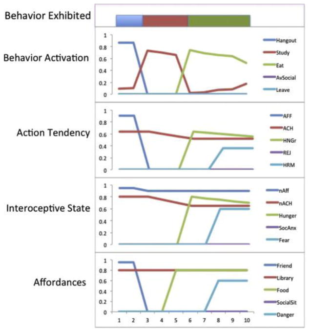
The three factors we focused on in building our model are: (1) environmental affordances, (2) interoceptive states, and (3) competition between alternative possible action tendencies and actions, as illustrated in Figure 1. The environmental affordances we examined were Friend, Library, Food, Social situation, and Danger. The interoceptive states were need for affiliation (nAFF), need for achievement (nACH), hunger (HNGr), social anxiety (SocAnx) and fear (Fear). The action tendencies were Affiliation, Achievement, Satisfy hunger, Avoid rejection, and Avoid harm. And the behaviors were to Hangout, Study, Eat, Avoid social interactions, and Leave.

Figure 1.

From Read, Smith, Droutman, and Miller (2017, Figure 5). “Results of simulation of the role of 3 factors over time. Affordances and Interoceptive State line graphs represent the inputs to Action Tendency in the network at each time step, where time is on the x axis. The Action Tendency line graph represents the result of multiplying Affordances by Interoceptive State and the resulting activation for each corresponding Action Tendency. The Behavior Activation line graph represents the resultant activation of the different behavior nodes in the Behavior Layer, after competition between the nodes in the layer. The Action colored bar represents the winning Behavior, at each time point. (For interpretation of the references to colour in this figure legend, the reader is referred to the web version of this article.)”

Read, Smith, Droutman, and Miller (2017) showed in their neural network simulations that variations in these 3 factors produced variability “under the skin” within a virtual personality (VP), and this underlying personality dynamic resulted in a VP’s variability in exhibited behavior over time. Furthermore, Read, Smith, Droutman, and Miller (2017), were also able to exhibit individual differences within this extended model. For example, variability in time to feeling satiated (e.g., by food) produced differences in time spent in an activity (e.g., eating versus studying), all else held constant (Figure 2). Alternatively, individuals may vary in their sensitivity to threat, with resultant individual differences in chronic outcomes likely. For example, if VP2 has higher threat sensitivity than VP1, VP2, given the situations possible in the simulation, is more likely to leave when there is a danger and stop studying compared to another VP with lower chronic sensitivity to threat. (Figure 3).

Figure 2.

(see From Read, Smith, Droutman, and Miller (2017, Figure 6). “Impact of slower rates of satiation on behavior choice [Compared to Figure 1]. Affordances and Interoceptive State line graphs represent the inputs to Action Tendency in the network at each time step, where time is on the x axis. The Action Tendency line graph represents the result of multiplying Affordances by Interoceptive State and the resulting activation for each corresponding Action Tendency. The Behavior Activation line graph represents the resultant activation of the different behavior nodes in the Behavior Layer, after competition between the nodes in the layer. The Action colored bar represents the winning Behavior, at each time point. (For interpretation of the references to colour in this figure legend, the reader is referred to the web version of this article.)”

Figure 3.

From From Read, Smith, Droutman, and Miller (2017, Fig 7.) “Simulation of greater sensitivity or gain to threat [Compared to Figure 1]. Affordances and Interoceptive State line graphs represent the inputs to Action Tendency in the network at each time step, where time is on the x axis. The Action Tendency line graph represents the result of multiplying Affordances by Interoceptive State and the resulting activation for each corresponding Action Tendency. The Behavior Activation line graph represents the resultant activation of the different behavior nodes in the Behavior Layer, after competition between the nodes in the layer. The Action colored bar represents the winning Behavior, at each time point. (For interpretation of the references to colour in this figure legend, the reader is referred to the web version of this article.)”

4. Developing The Theory That Led To The Read, Smith, Droutman, & Miller (2017) Model

A clear theoretical idea of the process or phenomena one intends to model is the key starting point for building a neural network model (or any computational model). Building a neural network model will not take the place of non-existent or sloppy theory. Once the theory has been specified, one needs to be quite clear on: (1) the inputs to the model, (2) the nature of the mediating elements and how they are represented, (3) the processes operating on the elements, and (4) the output of the model. All of these things need to be established before one can build the model. While one’s theoretical model might change in the process of building the neural network model, as some theoretical issues are clarified, one should not use the model building process as the start of one’s theoretical development.

In the current model of within subject variability in personality related behavior, we first had to clearly lay out our theoretical assumption about how to think about personality, how to think about situations, and how to think about how those two things are combined to result in behavior over time in different situations. Without a specific, clear idea of how to think about these two concepts, it is impossible to implement them in a neural network (or any kind of computational) model.

First, following our earlier work (Miller & Read, 1987, 1991b, 1991a; Read et al., 2010; Read & Miller, 1989), we argue that an important component of personality traits is the person’s underlying motives and that individual differences are largely based on individual difference in the chronic importance or activation of these motives. Read, Droutman, and Miller (2017) simulated an “army” of virtual personalities, where the resultant VP data simulated across individuals showed how structured motivational systems could produce the Big Five personality structure. A central distinction is between approach and avoidance motivational systems. There is considerable theoretical and empirical justification for arguing for universal approach and avoidance motivational systems(C. Carver, 2006; C. S. Carver & White, 1994) with an approach system governing reward and the avoid system governing punishment sensitivity(Gray, 1982; Gray & McNaughton, 2000). Moreover, there is considerable work suggesting that individual differences in these two motivational systems are related to two major dimensions of personality: Extraversion and Neuroticism. Thus, based on these and related theoretical assumption, to build the model one needs to explicitly represent the different motives and to organize them into two motivational systems.

Second, we have long argued (Miller & Read, 1987, 1991b, 1991a; Read et al., 2010; Read & Miller, 1989; Y. Yang, Read, & Miller, 2006, 2009; Yu Yang et al., 2014) that an important component of a situation is the goals or motives that can be achieved in that situation (its affordances). Sherman et al. (2015) found considerable between subject variability in situational affordances and also demonstrated that situational affordances vary considerably over time, with within-person variability greater than between subject variability. These situational affordances will activate their corresponding motives. Thus, different situational affordances need to be explicitly represented as part of the inputs to the model.

Following from these analyses of person and situation, person-situation interactions can be viewed in terms of the interaction between individuals’ active motives and the motive affordances of the situations in which they find themselves. These person-situation interactions should be captured by how the situational affordances are connected to or “wired” to the relevant motives. One must provide an explicit account of how these two elements interact.

Third, we have recently added an additional component to our theoretical model, bodily or interoceptive state, which is critical in understanding an individual’s degree of wanting for something. Interoceptive state was added to the Read, Droutman, and Miller (2017) paper in response to work by Bechara (Bechara & Naqvi, 2004) and Berridge (Berridge, 2012; Berridge & O’Doherty, 2013) that supported the claim that wanting for something is a multiplicative function of both cue strength (i.e., the strength of the affordance) and the animal’s cue-relevant bodily state. Therefore, the strength of wanting for food (or social interaction) depends on one’s current state such as hunger (or loneliness) as well as the cue strength of the food (or attractiveness of the other).

For example, WANTING food would be the result of a multiplicative function of how attractive a food is and how hungry we are. Something like this multiplicative rule needs to be implemented in the network model. Further, the degree of wanting will also be influenced by chronic differences in the importance of the relevant motive, which also has to be explicitly represented.

Fourth, we propose that competition among different WANTINGS and among different behaviors plays an important role in behavior. Many times we want multiple things, but we can’t pursue all of them at once. And we typically have to behave in a largely serial fashion. This process of competition needs to be part of the model.

Finally, an important part of the conceptualization task is specifying the dynamics that may produce emergent change over time. That is, “why (and how) does an organism’s need for food or social contact vary over time?” It is clear that as an individual behaves over time their behavior can lead to satiation of needs: as we eat our hunger goes down, as we hang out with friends our need for social affiliation goes down. Conversely, being alone for a while can lead to increases in need for social affiliation. Thus, the impact of behavior on internal bodily state must be taken into account.

Further, behavior can lead to changes in the situation; such as the consummation and reduction in the availability of goal objects, e.g., as we eat the amount of food goes down. Or conversely, moving into a new situation can make new affordances available and others unavailable. Thus, the effect of behavior on the environment must also be part of the model.

How changes in behavior are expected (given research and theory) to impact components of the model must be carefully conceptualized (with a process diagram specifying links between components, and preferably with hypothesized mathematical functions) at this point (e.g., this much of a change in x will produce this much of a change in y). Thus, conceptualizing the model requires the ability to “think dynamically” about persons and situations and how the key underlying components (e.g., affordances, action tendencies, bodily state) might change over time as well as the implications of those changes for what might happen next in the system.

What does it mean to “think dynamically”? An example may best help explain this. Personality psychologists are quite comfortable with the thought, “personality motive x₁ predicts behavior y₁” or even that there might be a moderator operating -- this happens under z₁ circumstance but not z₂ circumstance. Here, the x, y, and z are described in a fairly static way. When we think descriptively and in a fairly static way, the situation and its features (and affordances) are not presumed to be changing and competing for our attention (and thereby affecting changing motive activations). Such a static model cannot properly describe ways that our decisions and actions change the situational features, which in turn affect our now current motive activations (and competition among them) in driving decisions and actions. However, when we think about how to model ongoing social interactions, including the two-way causal links typically present between an individual and their situation during a social interaction – e.g., during a conversation – then we start thinking more dynamically. A better model of psychological systems must describe change and flux in the underlying competing motives guiding behavior and how they are influenced by what’s happening and changing within our bodies and in the world around us.

Once your theoretical assumptions are clearly laid out, it is usually important to develop a concrete instantiation or example of your model. For example, if you intend to take the above theoretical model and turn it into a neural network model of within subject variability in personality related behaviors over time and situations, it is important to create what one might think of as a model system, such as a college student behaving over the course of a day. In many cases building a purely abstract model wouldn’t make a great deal of sense to one’s reader (or even to oneself) and even when it does, a concrete example makes it easier to think about what is going on.

Here you would identify the typical kinds of situations the student might encounter, the affordances of those situations, relevant motives, relevant bodily states and the behaviors that might be enacted in the service of those motives. Based on our past experience in building models, we suggest that one should not be exhaustive but should only be detailed enough to provide a convincing model. Too much complexity makes a model difficult to build, debug, and comprehend.

4.1 The STUDENT Model

We demonstrate our multiplicative model of human motivation, in the context of a ‘day in the life of a college student’ as a way to set out a concrete example of human motivation in everyday life. Here, we could identify a set of motives that could plausibly explain behavior over the course of a day. Of course, the model is necessarily reductionist and excludes a number of complexities that would be present in real life, but we believe the model explains a substantial portion of behavioral patterns in a way that explains individual differences and changes in behavior over time. We settled on several needs: hunger, achievement, social affiliation, social anxiety, and harm avoidance. In a simple model, each of these needs can be matched one-to-one with commensurate situational affordances – food, a study environment (e.g., a library), friends, a potential partner, and danger. Similarly, these can all be mapped to resultant behaviors: Eat, study, hangout, avoid socializing, and leave. To demonstrate this in a compelling way, we present a dynamic model where behavior changes as a response to changes in needs and situations over time.

In this section, we describe how to plan the representation of a model in clear forms that can be implemented using computer software. We will take the concepts from our student model example described in the previous section, and discuss how we can translate those into a model representation. In the previous section, we identified several concepts necessary for the model: affordances (situations), interoceptive state (needs), action tendencies, and resulting behavior. We also described how a multiplicative relationship exists between situations and needs to produce action tendencies and resulting behavior, and how approach and avoid systems, as reward and punishment sensitivity, work together to produce behaviors. Additionally, to represent qualitatively different human needs, situations, and behaviors, we need a way to represent each of them within the system.

In order to plan a model for this system, we start with the core concepts, represented symbolically, and extend the model with each additional feature we wish to integrate.

In our student model of motivation, the core concept, a multiplicative relationship between needs, situations, and behaviors, can be represented symbolically,

$$\mathbf{b}=\mathbf{n}\times \mathbf{s}$$

where b, n, and s are vectors representing behavior, needs, situations, respectively. These must be vectors because, as described above, we model multiple behaviors, needs, and situations. We have stipulated that there is a one-to-one relationship between behaviors, needs, and situations – one need combines with only one particular situation to produce one particular need, so the multiplicative relationship could be represented as simple vector multiplication.

Behaviors change both remaining needs and the environment: eating helps to satiate hunger, and running from danger can reduce risk in a given situation. Even though strictly speaking, these are changes outside of a psychological model, we need to take them into account if we wish to dynamically represent needs, situations, and behaviors. Furthermore, these effects can only be measured over time; eating now only reduces hunger after ingestion of food, so a dynamic, time series model is necessary. So in the model, we represent each value with respect to a particular point in time, and describe how performing a behavior at a particular moment will change the experienced bodily state in the next moment (satiation):

$$n[t+1]=n[t]-r_n$$

and change situational features:

$$s[t+1]=s[t]-r_s$$

where r is the satiation or consumption rate at each point in time¹ t. As described in the previous section, the dynamic approach illustrated here, where we can calculate bodily state and situational features at different time points, allows us to cleanly illustrate how behaviors arise from different situations and states over time, and how an organism can move from one activity to the next. By functioning as a simulation of human behavior, the model can represent a human phenomenon such as declining marginal utility, and resolve a number of psychological controversies, such as reconciling the concept of personality with critiques that center on context as the key to differences between individuals’ behavioral patterns. In our dynamic model, stable individual differences in behavioral patterns can arise from simple individual differences like variations in various psychological needs as well as continuous variations in environmental situations.

As described above, in this model, we also wish to represent how personality structures defined by approach and avoid tendencies systematically change behavior. With the needs we have chosen to model, we can make the simplifying assumption that each need and consequent behavior is associated with either approach or avoid motivation. To do this, we can represent approach and avoid action tendencies, activated by needs and situations that compete to produce behavior, replacing the first equation with the following set of equations:

$$\begin{gathered} {\mathbf{a}}_{+}={\mathbf{n}}_{+}\times {\mathbf{s}}_{+} \\ {\mathbf{a}}_{-}={\mathbf{n}}_{-}\times {\mathbf{s}}_{-} \\ {\mathbf{b}}_{+}={\mathbf{a}}_{+}+{\mathbf{a}}_{-} \end{gathered}$$

With small modifications, such as adding a weight to each of approach and avoid parameters a₊, and a₋, we can calculate relative influences of approach and avoid orientations.

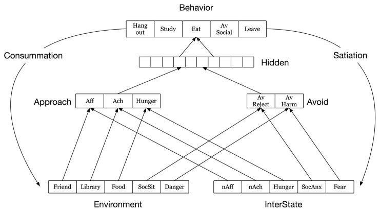
With these mathematical representations, we have, in principle described all of the framework necessary to run the model analytically. It is also critical to develop a visual representation of the elements and how they are connected or “wired together” (shown here in Figure 4), using software for developing flow charts or organization charts, such as the drawing package in PowerPoint or packages such as OmniGraffle on the Mac or Visio on Windows. It is much easier to build and modify these models in software designed for this purpose, than in a neural network package that is not optimized for drawing flowcharts. We have also found these kinds of visual representations to be quite helpful in clarifying one’s theoretical assumptions and in trying out alternative possibilities before make the greater commitment to actually building and then running the model.

Figure 4.

Structure of the model to be represented.

We can then use the conceptual analysis to this point and the visual diagram to plan our network. We need the following layers in the network. For the inputs, we need a Situation or Environment layer to represent the motive affordances in the Environment, where each node corresponds to a different affordance and an Interoceptive state (InterState) layer to represent the bodily state, where each node represents the current level of a different bodily state. These two layers then send activation over a set of weights to separate Approach and Avoid layers, where the nodes in each layer represent the degree of Wanting for each object or action. The layers need to be able to calculate a multiplicative result from the inputs from the Environment layer and the Interoceptive state layer. To insure that the Wanting for a specific thing is only a function of the corresponding nodes from the Environment and Interoceptive state layers, we need to make sure that there are one to one connections from each affordance and bodily state node to their corresponding Wanting node. There are separate layers for the Approach and Avoid system to represent the idea that they are separate motivational systems and relatively independent from each other, whereas there is considerable competition within each of the layers. After the Approach and Avoid layers, there is a Hidden layer that takes the inputs from the two layers and calculates a conjunctive representative from those inputs. Finally, there is a Behavior layer that takes the inputs from the Hidden layer and calculates the activation for each behavior node, which is a function of the inputs from the Hidden layer and the degree of competition among the behaviors. That is, there are six planned layers.

In addition to this network, we also need to think through how to capture the role of changes in both bodily state (InterState) and the Environment in subsequent processing in the network. Both bodily state and the Environment will change over time: for example, if you haven’t eaten for a while you get hungry or people may enter and leave the environment. Further, one’s actions can change these things: you eat and get less hungry, you leave the scene and people are no longer around. In the current example, we do not provide details of how that is implemented in emergent as that takes several pages of programming code “behind the scenes” to capture how bodily state and the environment can change with the passage of time and in response to the actor’s behavior. However, these “behind the scenes” changes play an important role in behavior.

Once this conceptualizing and planning have been done, we can then build the model in the appropriate software, in this case the Leabra architecture (Aisa, Mingus & O’Reilly, 2008) within the emergent neural network modeling system.

4.2 Building the Neural Network

The emergent neural network software package, which includes the Leabra architecture, is available at: https://grey.colorado.edu/emergent/index.php/Main_Page Leabra stands for Local, Error-driven and Associative, Biologically Realistic Algorithm. It is an attempt to build a biologically plausible neural network architecture that is still at a useful level of abstraction and does not try to get down into the specific details about things such as the neurophysiology of individual neurons. Downloads and instructions for Windows, Mac, or Ubuntu are available at this site. This tutorial will make the most sense if the reader first downloads and installs the software and then follows along with her or his own copy. There is also documentation and a number of tutorials, both video and written.

The steps for creating a network for the above model are as follows.

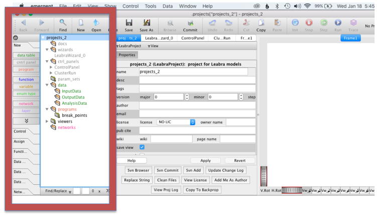
1. Start program and Create new project. From the top menu (Figure 5) select File -> New Project. Select LeabraBlank project template from the popup list and click ‘Ok’. A new project will be created and its structure shown in the left panel. (Figure 6). Click on the project name and its properties will be displayed in the middle panel where you can change name and other descriptive information (Figure 6).

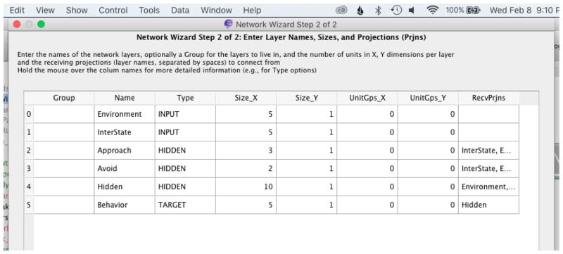
2. Use the wizard to configure model layers and projections. Click on LeabraWizard_0 in the left panel (Figure 6), wizard information will appear in the middle panel (Figure 7). Scroll down and click on Standard Network. In the Wizard Step 1 window that opens set the number of layers to 6 (which follows from our earlier planning and the diagram we developed) and press ‘OK’. The Network Wizard Step 2 window (Figure 8) will then open that allows configuring the network layers and their projections. Edit the layer configuration as shown in Figure 8

   You use this window to Name each layer, indicate its Type (defined shortly), give the Size of the layer (x * y nodes), and the layer(s) from which the layer receives projections (RecvPrjns column). (UnitGps_X and UnitGps_Y can be ignored for now). The Type of the layer is very important as it indicates whether it is a layer that is responsible for input (INPUT), whether it is an output layer that receives a teaching signal (TARGET), or whether it is a layer that does internal processing (HIDDEN). Different types of layers do different kinds of processing so it is important to be accurate in specifying the correct type.

   While configuring the layers, make sure that the following projections are set up in the RecvPrjns column, which indicates where the connections come from: “Approach” and “Avoid” layers receive projections from “Environment” and “InterState” (partially hidden in the figure), the “Hidden” layer receives from all 5 other layers (partially hidden in the figure) and the “Behavior” layer receives from “Hidden”. In setting up the projections make sure that you use the Names you defined in the Name column and not the Type. Once you are finished click OK, which is not visible in Figure 8, but which is lower on the figure.

3. Use the LeabraWizard to create Input/Output tables. Go back to LeabraWizard_0 (Figure 7) and click on StandardData. In the resulting dialog box set number of patterns to your desired number. This will create the DataTables with the desired number of rows that will hold the training and testing stimuli (InputData), as well as the outputs of various statistics during training and testing (OutputData).

4. Use the LeabraWizard to create Training programs and separate Testing programs. Create Training Programs by clicking on StandardPrograms in the LeabraWizard_0 (Figure 7) to create training programs, and then click on Programs button and select Test Prog to create testing programs. The training programs are a set of programs that are used to apply training instances to the network, settle the networks, and then record various statistics from the network, such as the activations for the Behavior layer or the error of prediction, into the OutputDataTables. The testing programs are a separate set of programs for testing the network after it has learned.

5. Adjust layer position on the network graph. It will be helpful to adjust the layer position on the network graph (Right panel) (Figure 9) to better represent the layer’s functionality. To do so you can either move the layers directly on the graphic panel or click on the layer you want to move and adjust the coordinates (that will be displayed in the middle panel). For example click on the Avoid layer and change the x, y, z coordinates (pos abs line) to (10, 0, 2), to set it on the same level with the Approach layer. To move layers directly, first press the red arrow in the top right corner of graphic panel which will activate interaction mode; you will now be able to move the layers by dragging on the ‘handle’ (light purple arrows that now appear on the front left corner of each layer).

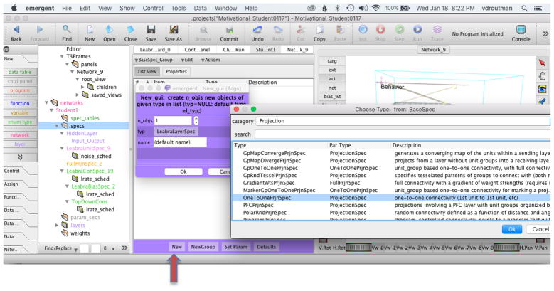
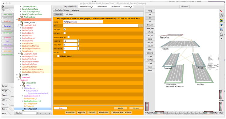
6. Change Projection Type. Next we will change projection type from the input layers (Environment and InterState) to Approach and Avoid from Full projection to One-to-One projection (Full projection, which connects each node in one layer to each node in the other layer is the default). One-to-One projections connect each node in the sending layer to only one node in the receiving layer. We do this so that activation from each Affordance (e.g., food) node will only be multiplied by the activation from the corresponding Interstate (e.g., Hunger) node. We will first create two custom projection specs, one to Approach and one to Avoid layers. In the left most panel select specs and click ‘New’ button on bottom of the middle panel (Figure 10). Click on the type, in the selection window choose category ‘Projection’ and type ‘OneToOnePrjnSpec’ and press ‘Ok’. In the resulting dialog box (Figure 11) change name to ‘PrjToApproach’, make sure that recv start and send start are set to 0, and press Apply. These indices will ensure that the connections start with the first node (0) in the sending layers (Environment and InteroState) and the first node (0) in the receiving layer (Approach). Counting typically starts with 0 in emergent. Create another OneToOne projection ‘PrjToAvoid’ and set recv start to 0 and send start to 3 (you can do this by right clicking on the PrjToApproach and selecting ‘Duplicate’ option, then adjusting the name and send start). This setup insures that the last 2 nodes (3 & 4, starting from 0) on the Environment and InterState layers project to the corresponding nodes in the Avoid layer. Overall this setup insures that there is a one to one relationship such that each unit from the input layers can only send activation to one specific unit on the Approach or Avoid layers.

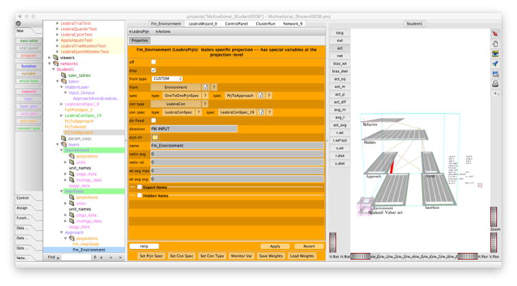
   Now change projection specs for the Avoid and Approach layers to the new projection specs we just created. To do so select the projection to Approach from Environment either by clicking on it on the graphical panel or on the left most panel scroll to the Approach layer and select Fm_Environment projection. In the Properties (central) panel (Figure 12) set the type to OneToOnePrjnSpec and select PrjToApproach spec. Repeat this process to set Fm_InterState spec and both specs to Avoid layer.

7. Modify Approach and Avoidance Layers. In order to achieve ‘multiplicative-like’ projection from input layers to Approach and Avoid layers we will create a custom layer spec for the two layers with fixed inhibition set relatively high. Among other things, the layer spec controls how much inhibition there is among the nodes in the layer. High inhibition will insure that a node can only become activated if it receives large amounts of activation from both inputs. Thus, it will behave as if there is a multiplicative (or gating function) between the affordances in the Environment and the InterState. In the navigation (left) panel (Figure 13) locate the Spec section of the network, select on Input_Output under HiddenLayer; on the bottom of the properties (middle) panel click on the ‘New Child’ button. Leave child_type as default LeabraLayerSpec and change the name to ApproachAvoidLayer and press ‘Ok’. Set the new child spec as follows. On the field labeled “lay inhib” set gi to 2 and fb to 2. This will increase the level of inhibition in the layer. Now change the layer spec on Approach and Avoid layers to the newly created ApproachAvoidLayerSpec.

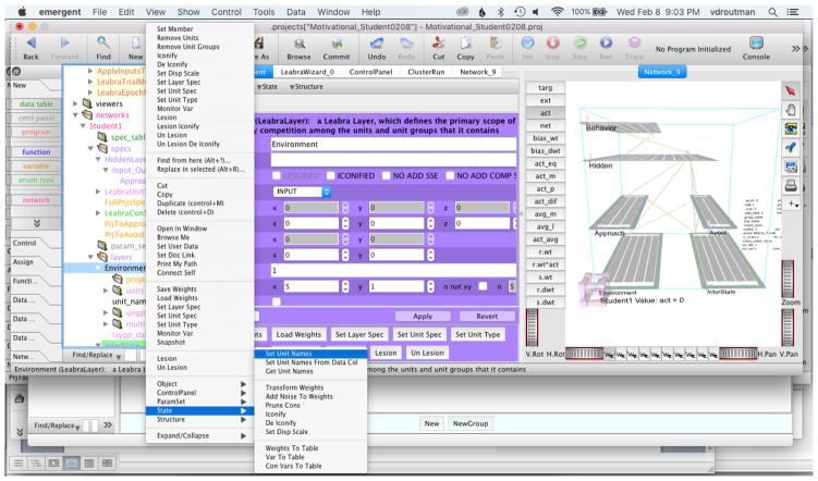
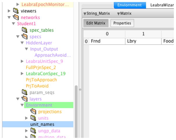
8. Name units. Find the layers in the navigation (left) panel and right-click (or Control-click for the Mac) on the name of the layer for which you want to assign unit names (Figure 14). For instance, right click or Control click on the Environment layer. A menu will appear and near the bottom of the menu will be a choice “State”. Choose that and then in the next menu Choose “Set Unit Names.” In the resulting dialog box, click on the “force_use_unit names” check box and then click on “OK”. Once you have done that, click on the disclosing triangle next to the Environment layer name (Figure 15). You will see “unit_names.” Click on “unit_names” and you will then see a data table in the middle panel. You can enter names for each node in the corresponding cells.

   Once you have entered the names, to make the names appear on the network diagram in the right hand panel you need to do two things: (1) go to the tree browser in the left hand panel and click on the name of the network. In this example, it will be Student1. You will see a dialog box in the middle panel that has a number of options. At the bottom of the panel, you will see a number of buttons. Click the one that says “Build” to build the network. (2) Then in the middle panel (Figure 16), click on the last tab, which will bring up a panel that controls the display characteristics of the network (Network_9 in this example). In the resulting dialog box in the middle panel, set “Net Unit Txt.” to ‘Names.’ The Unit names you entered should now display on the network diagram in the right-hand panel.

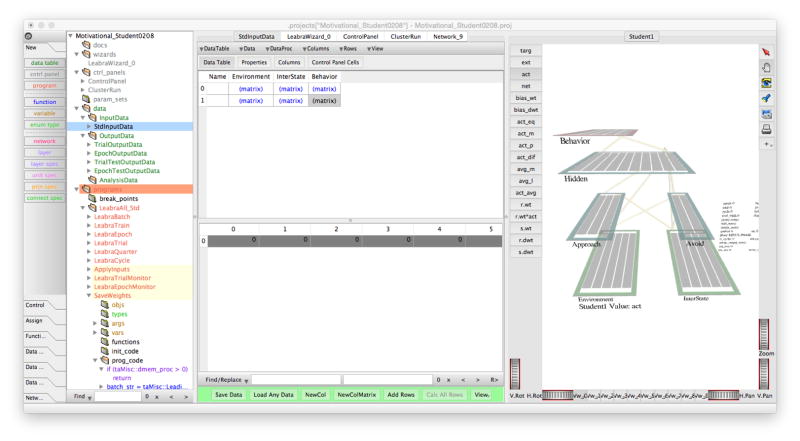
9. Enter data into InputDataTable. At this point you can then enter data into the Input Data Table for training and testing purpose. Go to the left browser window and go up to InputData (Figure 17). Under that you will see StdInputData. Click on that and you should see a spreadsheet in the middle panel. If you click on one of the cells, you will see a set of cells in the bottom of the panel. You can enter data manually here or you can have the program read in data from a properly formatted data file, such as a csv file.

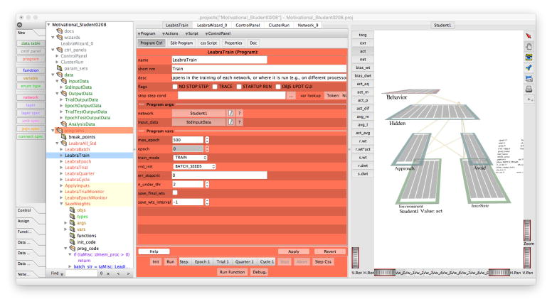
10. Run the program. Once you have the data entered you can then go to the left panel browser to run the program. In the Program list, click on LeabraTrain program (Figure 18). In the dialog box in the middle panel you can now run your program. In the dialog box are several options for controlling things like the number of passes through training and which data files to read from. At the bottom of the dialog box are buttons that say Run and Init. Pressing the Init button will initialize your network and programs. Clicking Run, will start training the network.

11. More information. More detail about the program and its interface can be found on the tutorials page, which has a number of video and text tutorials: https://grey.colorado.edu/emergent/index.php/Tutorials and on the documentation page: https://grey.colorado.edu/emergent/index.php/Using_emergent

Figure 5.

Create New Project

Figure 6.

Initial project window

Figure 7.

Wizard information window

Figure 8.

Layer configuration window

Figure 9.

Initial Network Configuration graph, right panel

Figure 10.

Creating OneToOne projection spec.

Figure 11.

Set up new OneToOne projection spec

Figure 12.

Assign new projection specs for the projections to the Approach and Avoid layer.

Figure 13.

Creating custom layer spec for Approach and Avoid layers.

Figure 14.

Setting program to use unit names

Figure 15.

Entering unit names.

Figure 16.

Set unit names to display.

Figure 17.

Setting up the Input Data Table

Figure 18.

Running the program

5. Conclusion

5.1 Testing The Model Against Data

Currently, we are planning to test the model against real world data by collecting longitudinal data over a few weeks from undergraduate students using ecological momentary assessments (EMA) using well established procedures and insuring that we have reliable measures of the constructs used in the current example. For example, we would include assessments of variables that we would want students to record over time (e.g., relevant motives; relevant behaviors; relevant interoceptive states; etc.) that we will need to run our model. Here our model is not intended to literally be diagnostic of a given student’s sequence of behavior at a given time, but rather to illustrate that individuals may have a great deal of within person variability in their behavior over time and yet exhibit quite a bit of between subject variability as well. So our “fit” is a fairly loose criterion here. However, one could have a more specified model with a much tighter fit to a specific pattern of real-life behavioral outcomes expected via the model. For example, one might expect that where individuals have fewer activated and competing motives we might see more consistency in behavior across situations as well as stability (given similar situational patterns) over time. Or, when situational features are changing more, and/or these are more competitive, we might expect less cross-situational consistency in behavior and where habits are dependent on situational constraints, less stable exhibition of habit related behavior over time. Our computational models, with unexpected behavioral pattern outcomes especially, can also guide the questions to ask of real-life behavioral patterns. Needless to say, computational models such as these provide a way to develop a theoretical model against which to generate and test predictions in increasingly more complex observed patterns of ongoing, dynamic, “big data” in the future.

Although we probably cannot do precise model fitting, we can also use the model to generate some specific predictions. For example, we can explicitly test the idea that measured bodily states predict the strength of action tendencies and behavior and we can further test whether there is a multiplicative or some other kind of interactive relationship between situational affordance and interoceptive state in predicting motivated behavior.

5.2 Constraints and Limitations

In every model one builds one must be cognizant of the assumptions, constraints, and limitations one is “building in.” In the model we built we chose to simplify considerably what wasn’t a focus of the modeling effort. So for example, there was one link between an environmental feature and a motivational state. In real life, an environmental feature might concurrently send activation to a number of motives. If that was the focus of interest, a model could be built to examine the implications of that for behavior choice patterns. Researchers always make simplifying assumptions, and have resultant constraints and limitations as a result. But, with modeling it is necessary to be more consciously, and explicitly, aware of these decisions.

5.3 Next Steps

So what are the next steps to take if you are interested in learning more about constructing a neural network model of a psychological process? We have several suggestions. Assuming you haven’t already downloaded and installed the emergent software, we suggest that you do so. Once you have done that, there is a considerable amount of documentation about emergent at https://grey.colorado.edu/emergent/index.php/Main_Page, including video tutorials and written documents. In addition, there is a free textbook available on the website at https://grey.colorado.edu/CompCogNeuro/index.php/CCNBook/Main, which takes a cognitive neuroscience approach to a number of different aspects of cognitive processing and is an excellent introduction to the Leabra neural network architecture. Available with the book are a number of excellent example programs that provide models of a number of cognitive phenomena in areas such as perception, attention, working memory, episodic and semantic memory, and language. In addition, there is a voluminous literature on neural network models, but some good overview textbooks are the original PDP Handbooks(McClelland, Rumelhart, & PDP Research Group, 1986; Rumelhart, McClelland, & PDP Research Group, 1986) and a textbook by Bechtel and Abrahamsen (2002)).

In addition to the suggested readings and exercises, another critical thing is to actually build models. Just as you never learn statistics until you analyze data (preferably your own), you don’t really learn to model until you start building your own models. You can start by trying to replicate already existing models, but ultimately you need to start building your own model(s). Our advice is to start with a relatively simple model and as your model building skills improve move onto more sophisticated models. Avoid starting with a complex model, as this is a recipe for frustration and discouragement. Start with success and build from there. You will encounter enough barriers as you move toward more sophisticated and complicated models.

References

- Aisa B, Mingus B, O’Reilly R. The Emergent neural modeling system. Neural Networks. 2008;21(8):1146–1152. doi: 10.1016/j.neunet.2008.06.016. [DOI] [PubMed] [Google Scholar]
- Bechara A, Naqvi N. Listening to your heart: interoceptive awareness as a gateway to feeling. Nature Neuroscience. 2004;7(2):102–103. doi: 10.1038/nn0204-102. [DOI] [PubMed] [Google Scholar]
- Bechtel W, Abrahamsen A. Connectionism and the mind: parallel processing, dynamics and evolution in networks. 2. Malden, Mass: Blackwell; 2002. [Google Scholar]
- Berridge KC. From prediction error to incentive salience: mesolimbic computation of reward motivation. European Journal of Neuroscience. 2012;35(7):1124–1143. doi: 10.1111/j.1460-9568.2012.07990.x. [DOI] [PMC free article] [PubMed] [Google Scholar]
- Berridge KC, O’Doherty JP. From Experienced Utility to Decision Utility. In: Glimcher PW, Fehr E, editors. Neuroeconomics, Second Edition. Decision Making and the Brain. Academic Press; 2013. pp. 325–341. [Google Scholar]
- Carver C. Approach, Avoidance, and the Self-Regulation of Affect and Action. Motivation and Emotion. 2006:105–110. [Google Scholar]
- Carver CS, White TL. Behavioral inhibition, behavioral activation, and affective responses to impending reward and punishment: The BIS/BAS scales. Journal of Personality and Social Psychology. 1994;67:319–333. [Google Scholar]
- Fleeson W. Toward a structure-and process-integrated view of personality: Traits as density distributions of states. Journal of Personality and Social Psychology. 2001;80(6):1011. [PubMed] [Google Scholar]
- Fleeson W, Gallagher P. The implications of Big Five standing for the distribution of trait manifestation in behavior: fifteen experience-sampling studies and a meta-analysis. Journal of Personality and Social Psychology. 2009;97(6):1097. doi: 10.1037/a0016786. [DOI] [PMC free article] [PubMed] [Google Scholar]
- Gray JA. The neuropsychology of anxiety: An enquiry into the functions of the septo-hippocampal system. Oxford: Clarendon press; 1982. [Google Scholar]
- Gray JA, McNaughton N. The neuropsychology of fear and anxiety. Oxford: Oxford University Press; 2000. [Google Scholar]
- McClelland JL, Rumelhart DE PDP Research Group. Parallel distributed processing: Explorations in the microstructure of cognition: Volume 2: Psychological and Biological Models. Vol. 2. Cambridge, Mass: MIT Press; 1986. [Google Scholar]
- Miller LC, Read SJ. Why am I telling you this?: Self-disclosure in a goal-based model of personality. In: Derlega VJ, Berg J, editors. Self-disclosure: Theory, research, and therapy. Plenum Press; 1987. [Google Scholar]
- Miller LC, Read SJ. Inter-personalism: Understanding persons in relationships. In: Jones W, Perlman D, editors. Perspectives in Interpersonal Behavior and Relationships. Vol. 2. England: Kingsley Publishers; 1991a. pp. 233–267. [Google Scholar]
- Miller LC, Read SJ. On the coherence of mental models of persons and relationships: A knowledge structure approach. In: Fletcher GJO, Fincham F, editors. Cognition in close relationships. Hillsdale, N. J: Erlbaum; 1991b. pp. 69–99. [Google Scholar]
- Read SJ, Droutman V, Miller LC. Virtual Personalities: A Neural Network Model of the Structure and Dynamics of Personality. In: Vallacher RR, Read SJ, Nowak A, editors. Computational Social Psychology. New York: Routledge; 2017. pp. 15–37. [Google Scholar]
- Read SJ, Miller LC. Inter-personalism: Toward a goal-based theory of persons in relationships. Goal Concepts in Personality and Social Psychology. 1989:413–472. [Google Scholar]
- Read SJ, Miller LC. Virtual personalities: A neural network model of personality. Personality and Social Psychology Review. 2002;6(4):357–369. [Google Scholar]
- Read SJ, Monroe BM, Brownstein AL, Yang Y, Chopra G, Miller LC. A Neural Network Model of the Structure and Dynamics of Human Personality. Psychological Review. 2010;117:61–92. doi: 10.1037/a0018131. [DOI] [PubMed] [Google Scholar]
- Read SJ, Smith B, Droutman V, Miller LC. Virtual Personalities: Using Computational Modeling to Understand Within-Person Variability. Journal of Research in Personality. 2017;69:237–249. doi: 10.1016/j.jrp.2016.10.005. [DOI] [PMC free article] [PubMed] [Google Scholar]
- Rumelhart DE, McClelland JL PDP Research Group. Parallel Distributed Processing. Explorations in the Microstructure of Cognition: Volume 1: Foundations. Cambridge MA: MIT/Bradford Press; 1986. [Google Scholar]
- Sherman RA, Rauthmann JF, Brown NA, Serfass DG, Jones AB. The Independent Effects of Personality and Situations on Real-Time Expressions of Behavior and Emotion. Journal of Personality and Social Psychology. 2015 doi: 10.1037/pspp0000036. [DOI] [PubMed]
- Yang Y, Read SJ, Denson TF, Xu Y, Zhang J, Pedersen WC. The key ingredients of personality traits situations, behaviors, and explanations. Personality and Social Psychology Bulletin. 2014;40(1):79–91. doi: 10.1177/0146167213505871. [DOI] [PubMed] [Google Scholar]
- Yang Y, Read SJ, Miller LC. A taxonomy of situations from Chinese idioms. Journal of Research in Personality. 2006;40(5):750–778. [Google Scholar]
- Yang Y, Read SJ, Miller LC. The concept of situations. Social and Personality Psychology Compass. 2009;3(6):1018–1037. [Google Scholar]