Abstract
Purpose:
Magnetic resonance spectroscopy imaging (MRSI) has shown great promise in the detection and monitoring of neurologic pathologies such as tumor. A necessary component of data processing includes the quantitation of each metabolite, typically done through fitting a model of the spectrum to the data. For high-resolution volumetric MRSI of the brain, which may have ~10,000 spectra, significant processing time is required for spectral analysis and generation of metabolite maps.
Methods:
A novel deep learning architecture that combines a convolutional neural network with a priori models of the spectrum is presented. This architecture, a convolutional encoder – model decoder (CEMD), combines the strengths of adaptive and unbiased convolutional networks with models of magnetic resonance and is readily interpretable.
Results:
The CEMD architecture performs accurate spectral fitting for volumetric MRSI in patients with glioblastoma, provides whole-brain fitting in one minute on a standard computer, and handles a variety of spectral artifacts.
Conclusion:
A new architecture combining physics domain knowledge with convolutional neural networks has been developed and is able to perform rapid spectral fitting of whole-brain data. Rapid processing is a critical step toward routine clinical practice.
Keywords: MRSI, spectroscopic imaging, MR spectroscopy, brain, spectral analysis, machine learning, deep learning
Introduction
Proton magnetic resonance spectroscopic imaging (MRSI) is an imaging modality capable of generating high-resolution 3D maps of cerebral metabolites concentrations in vivo (1–3). Previous studies have shown that altered metabolism identified regions of occult tumor that are not visible in contrast-enhanced T1w MRI (3–5). Studies have assessed the potential of using MRSI to guide radiation therapy (RT) in patients with glioblastomas (6–9), and an ongoing multisite clinical study is prospectively boosting radiation based on this technique (NCT03137888, “Spectroscopic MRI-Guided Radiation Therapy Planning in Glioblastoma”) (10). To utilize volumetric MRSI for clinical studies, maps of the individual metabolite distributions must be created by quantifying the metabolite resonance peaks, a process known as spectral fitting. Several spectral fitting algorithms have been established, including ones that operate in both the time and frequency domain of the acquired data (11,12). Common amongst these techniques is the incorporation of prior knowledge, which includes information on the resonance frequencies of metabolites of interest and lineshapes. Several parametric spectral analysis methods have developed (13–19), all of which rely on iterative optimization procedures to find the model parameters that best match the data. However, these methods do not scale well to volumetric spectroscopic imaging, which can contain on the order of 10,000 spectra in a whole-brain scan. One method for processing of whole-brain MRSI is the FITT program of the Metabolite Imaging and Data Analysis System (MIDAS) (20,21), which uses iterative time-frequency parametric modelling methods for spectral analysis (15). This algorithm is typical of the parametric spectral analysis approaches that have been widely applied to MRS. As with other parametric spectral analysis methods, spectral fitting with MIDAS is computationally-intensive, requiring 40–50 minutes on a high-end multicore workstation. However, if MRSI is to be integrated into clinical protocols it is critical that all processing be done within a few minutes, ideally on board the scanner computer. This would enable rapid quality checks of the final maps to see if the scan needs to be repeated before the patient leaves and to be sent for clinical review in a timely manner.
Machine learning has proven to have exceptional utility in medical imaging, including MRSI (22–27). Hiltunen et. al. described an artificial neural network (ANN) architecture that could predict metabolite peak areas from magnitude spectra in patients with gliomas (26); Das et. al. presented a multi-layer perceptron (MLP) for quantifying metabolite concentrations from synthetically generated spectra and phase-encoded 2D MRSI using results from LCModel as data for supervised training, achieving accurate predictions of metabolite concentrations (28); and Bhat et. al. used an unsupervised neural network for analysis of phase-corrected 2D MRSI data (27). While these methods provide measures of metabolite concentrations, it is difficult to contextualize why the MLP or ANN produced a given output. A concept in machine learning that correlates well to curve fitting is the idea of the encoder-decoder, or autoencoder. Autoencoders are a type of unsupervised learning neural network that seek to find a compressed encoding of input data such that the input data can be accurately reconstructed from this parsimonious encoding (29,30). The autoencoder consists of two independent neural networks: an encoder, that transforms the input data into a lower dimensional space; and a decoder, that reconstructs the original input data from the lower dimensional representation (Supporting Information Figure S1). The encoder and decoder are concurrently trained to minimize reconstruction error, with the constraint that the interim representation has significantly lower dimension than the input, and thus only important “features” of the data are maintained. This process is highly analogous to parameterized curve fitting, wherein a model (the decoder) uses relatively few parameters to reconstruct a denoised version of raw data. With autoencoders, both the encoding and decoding models are neural networks (a cascade of convolution, pooling, matrix multiplication and summation operations) such that higher-order non-linear features can be extracted from the inputs. The model parameters of these neural networks can be optimized using gradient descent techniques to minimize reconstruction error. Generally, the only constraint on the autoencoder is the size of the lower dimensional representation, and as such, this low-rank representation is not readily interpretable.
To leverage the feature-learning capabilities of autoencoders while maintaining the interpretability of parameters given domain knowledge about MRS, a novel spectral fitting algorithm was developed that utilized a convolutional neural network encoder with a model-based decoding of the spectrum. We evaluated this method for fitting of singlet resonances in MRSI of the brain. We also implemented a software pipeline for rapid generation of metabolite maps of interest. Metabolite maps generated using this system were then compared with those produced by existing parametric spectral fitting methods.
Methods
Image Acquisition and Processing
Volumetric echo planar spectroscopic imaging (EPSI) scans were performed on four healthy subjects and six subjects with newly diagnosed glioblastoma who were enrolled in an ongoing clinical trial (NCT03137888). Scans were conducted at 3T (Siemens Prisma) with a 32-channel head coil (Siemens Healthineers, Erlangen, Germany). For the subjects with glioblastoma, data were obtained following surgical resection but prior to radiation therapy and chemotherapy, as previously described (23). Briefly, T1-weighted (T1w) magnetization-prepared rapid gradient echo pulse (TR = 1900 ms, TE = 3.52 ms, 256 x 256 × 160 matrix, flip angle (FA) = 9°) and whole-brain 3D EPSI (TR = 1551 ms, TE = 50 ms, 64 × 64 × 32 matrix, FA = 71°) sequences with generalized autocalibrating partially parallel acquisitions (GRAPPA) acceleration were obtained during the same scanning session, oriented at a +15 degree tilt in the sagittal plane from the anterior commissure-posterior commissure line (31). For the EPSI/GRAPPA sequence, an oblique saturation band was placed in the sagittal plane from the optic chiasm to the cerebellum. A medium TE of 50ms was used to reduce the impact of lipid contamination and emphasize the signal of metabolites of interest in subjects with brain tumors: choline (Cho), creatine (Cr), and N-acetylasparate (NAA). MIDAS (20,21) was used to perform the following preprocessing and volume reconstruction steps: spatial reconstruction, B0 field correction using simultaneously-acquired intracellular water signal, co-registration of the T1w and metabolite volumes, lipid suppression, and water suppression. The initial processing also created a mask covering the brain volume, but excluding voxels for which the water linewidth was greater than 18 Hz, as calculated using the T2* map. A total of 102,005 spectra were obtained and separated into three data subsets: 85,661 for training; 8,192 for validation; and 8,192 for testing.
For assessing generalizability, additional data from subjects with newly-diagnosed glioblastoma that were scanned at Emory University, the University of Miami and the Johns Hopkins University, were evaluated. The same sequences and parameters as above were used, with the exception that studies at the University of Miami were carried out on a 3T Siemens Skyra with a 20-channel head coil.
Convolutional Encoder – Model Decoder
The goal of spectral fitting for an input spectrum, , is to find a parameter set, such that when these parameters are used in a spectral model, g(θ), the result is a noise-free approximation of the input:
| #[1] |
Mathematically, this can be represented as the following optimization task:
| #[2] |
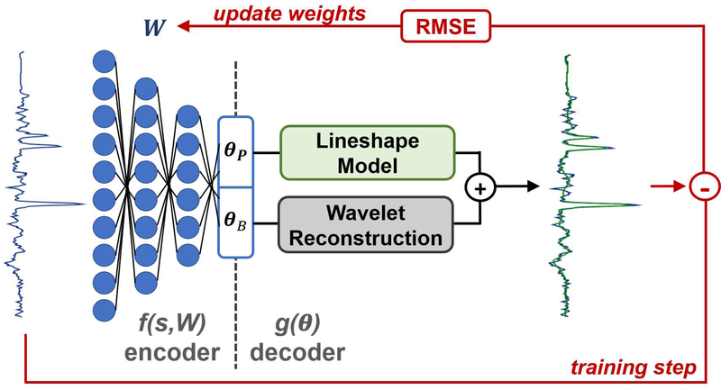
In this context, the task of finding θ is the encoding step while the function g(θ) is the decoding step. In this work, we define the convolutional encoder – model decoder (CEMD) architecture. The CEMD architecture is graphically depicted in Figure 1. The encoding step in CEMD is a convolutional neural network (CNN) composed of sequential layers of convolution, pooling, and rectification (32,33). Each of these layers is has parameterized weights that can collectively be referred to as W; therefore, the CNN with weights W can be conceived of as applying a series of transformations that perform the encoding function defined by f(s,W) = θ. Training identifies W to minimize the error defined Equation 2. In the context of spectral fitting, a fixed spectral model is used as the decoder (Equation 1) to generate a fitted version of the input spectrum. The overall training objective can be stated as:
| #[3] |
Figure 1.
Schematic of the convolutional encoder – model decoder (CEMD) architecture, which utilizes a convolutional neural network (CNN) to learn a low-rank representation of input spectra and uses known models for the baseline and peak components of spectra to train the CNN.
A key point in this optimization is that it requires no “ground truth” or “true” fitted spectra for CNN training. It is an unsupervised learning task requiring only a set of spectra, , to train the CNN weights with the goal of minimizing the residual error between the input data and fitted spectra.
The decoder was based on previously described parametric analyses that model a spectrum as having two components: i) metabolite resonances that are explicitly defined, and ii) a baseline composed of all metabolites and macromolecules not explicitly defined (14,15). Metabolite resonances were modeled using the Lorentzian-Gaussian lineshape model:
| #[4] |
For each metabolite, m, the metabolite model required six parameters: peak amplitude Am, resonance frequency ωm, zero and first order phases (ϕ0 and ϕ1), and Gaussian and Lorentzian decay constants (Ta and Tb). The three major singlet resonances at TE = 50 ms were modeled: Cho, Cr, and NAA. Note that this formulation returns the relative concentrations of each metabolite, not the peak area. A constraint was placed such that all three metabolites have the same zero- and first-order phase shifts and linewidths, such that only the resonance frequency and amplitude needed to be independently determined. Since the expected resonance frequency, defined as ωm,0, is known a priori from a library of chemical resonances, only a shift in frequency from the expected, Δωm, needed to be calculated. Thus, for these three metabolite singlet resonances, a total of 10 parameters were needed:
| #[5] |
The baseline component was defined by wavelet reconstruction, using a set of coarse (34) third-order Coiflets (35) as the wavelet kernels and four levels of dyadic upsampling to convert 32 coarse coefficients (θB) into the baseline signal. In order to enable automated computation of gradients for training the CNN in TensorFlow (36), wavelet reconstruction was implemented as a series of linear matrix operations. At each level, the output of the previous iteration, were first dyadically upsampled (37). Dyadic upsampling on a vector y was implemented as augmentation of its transpose with a vector of zeros of the same size, followed by vectorization and transposition:
| #[6] |
| #[7] |
| #[8] |
The upsampled vector was then convolved with the Coiflet low-frequency reconstruction kernel, Coif3low (35):
| #[9] |
The central 2p elements of y′low were used as the input for the next level of wavelet reconstruction. The CEMD encoder therefore needed to calculate 42 coefficients, 10 for the metabolite resonances and 32 for the baseline, which are passed to the decoder to create the fitted spectrum.
A more detailed representation of the CEMD architecture is shown in Supporting Information Figure S1. Only the real component of the complex input spectrum () was passed through a CNN during the encoder to produce a low-rank representation that directly corresponded to the 42 spectral model parameters. The decoder then applied the metabolite resonance and baseline models to the low-rank representation and created the fitted spectrum (). The training set consisted of N=85,661 frequency domain spectra each consisting of 512. The mean and standard deviation of the amplitude, μtrain and σtrain, were computed across the entire set, and each input spectrum, , was normalized as:
| #[10] |
While CEMD followed an encode-decode scheme, it consisted of two serial encoder-decoder stages. First, the normalized spectrum, , was passed through a CNN that computed the 32 coarse wavelet coefficients, θB. This CNN consisted of 13 convolution layers, with max-pooling after the 4th, 8th, and 13th layers, followed by two fully-connected (FC) layers (32,38). An estimate of the baseline, , was made from the decoder using the wavelet reconstruction technique described in Equations 5–9. Next, the baseline was subtracted from the input spectrum:
| #[11] |
The baseline-subtracted spectrum, , was passed through a second CNN consisting of just 6 fully-connected layers that computed the metabolite resonance peak parameters, θP. An estimate of the metabolite resonances, , was made by the decoder using Equation 4. Next, the baseline and resonance peak estimates were added together to produce an estimate of the fitted spectrum, The root-mean-squared error (RMSE) of the input and fitted spectrum was used to update the weights of the encoder CNN, and was calculated as:
| #[12] |
CEMD was developed in the Python programming language using the TensorFlow 1.3 (Google LLC, Mountain View, CA) library, and trained using TensorFlow’s Adam optimizer (39) on a high-end workstation with two Titan X graphical processing units (GPUs; Nvidia Corporation, Santa Clara, CA).
In each epoch of training, spectra in the training data set were run through CEMD to produce fitted spectra, RMSE for each spectrum was calculated, and gradient backpropagation was performed to update the encoder weights. Then, the spectra in the validation set were run through the CEMD and the validation loss was calculated as the sum of RMSEs. Training continued through multiple epochs until the validation loss converged. Once the autoencoder was trained and the CNN weights finalized, the testing set was used to determine final statistics of CEMD performance. The RMSE was calculated for each spectrum in the testing set, and the mean and standard deviation were reported. Once training of the CEMD encoder weights was complete, the encoder can be applied to spectra to compute the relative concentration of each metabolite resonance based on the parameters in the encoder output, θP.
Whole-brain Mapping
A software pipeline to perform CEMD fitting on whole-brain MRSI and to generate volumetric metabolite and ratios maps was developed. Only voxels within the region defined from the brain mask were analyzed, for both the CEMD and MIDAS fitting. While training of the CNN required a GPU, the final CEMD was implemented on a central processing unit (CPU) architecture consisting of a four-core CPU. To assess the utility of generated volumetric for radiation treatment planning, the Cho/NAA ratio map was computed for 10 subjects with glioblastoma fitted by CEMD and an existing parametric analysis method implemented in MIDAS. Spectral fitting in MIDAS used the METAFIT option, which applies three applications of fitting (the FITT program). First, B0 and phase corrections are performed, prior to applying a spatial smoothing and fitting of a higher-SNR copy of the data. Using the initial values from this intermediate result a final spectral analysis is performed on the original spectra. After fitting, voxels were excluded from both sets of results based on spectral outlier filters, namely those having values that are more than four standard deviations from the mean value within the brain.
Identification of abnormal Cho/NAA regions was determined from the results of each fitting method using the largest single connected component of voxels that had a Cho/NAA at least twofold increased compared to the mean value in contralateral normal-appearing white matter; this particular threshold was previously determined to be optimal for identifying high-risk regions for disease recurrence (3,10,40). The identified regions from each result were compared using the Dice similarity coefficient (DSC) (41) and a Z test was performed for each subject using the logit transform of the DSC (42).
Results
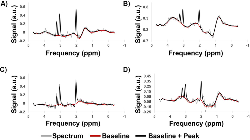
Training time for the CEMD was approximately 4 hours using TensorFlow on a workstation with two Nvidia Titan X GPUs. The testing set achieved a mean RMSE of fit of 5.0% normalized to the amplitude of the largest peak in each spectrum in the testing set, with a standard deviation of 0.6%. Sample spectra from the testing set are shown in Figure 2, with the baseline (red) and peak + baseline (black) fit overlaid on the input spectra (gray). CEMD can handle a variety of baseline effects, varying from a relatively flat baseline near the peaks of interest (Figure 2A) to major shifts that can occur at frequencies in the region of lipid or metabolites (Figure 2B). Phases can also be determined by the model (Figure 2C-D). Even if the signal-to-noise ratio is poor, due to partial volume effects, magnetic field inhomogeneity, or receiver coil sensitivity, CEMD can identify and fit the peak and baseline components.
Figure 2.
Example spectra generated by CEMD, showing the real components of the computed baseline (red) and baseline + peak (black) fits overlaid on top of spectra (gray). Four different types of baseline and phase shifts are shown to indicate that CEMD is able to handle a range of input spectra. a.u. = arbitrary units.
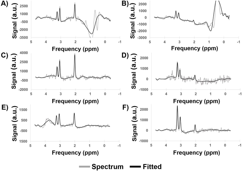
Sample spectra from three subjects with glioblastoma, not included in the training, testing, or validation sets, are shown in Figure 3. In patients with glioblastoma, voxels within the region of active tumor exhibit an increase in Cho and a concomitant decrease in NAA (3). The CEMD-fitted spectra (black) are overlaid on the input spectra (gray). Subject one (Figure 3A,B) was scanned at Emory University; subject two (Figure 3C,D) was scanned at the University of Miami; and subject three (Figure 3E,D) was scanned at the Johns Hopkins University. All three subjects were scanned using the protocol defined in the Methods section, and data were preprocessed in MIDAS as described. Spectra in the left column (Figure 3A,C,E) are from voxels in the contralateral normal-appearing hemisphere, while spectra in the right column (Figure 3B,D,F) are taken from voxels in regions of tumor.
Figure 3.
Sample spectra (real components) from scans of subjects with glioblastoma. Subject 1 (A,B) was scanned at Emory University; subject 2 (C,D) was scanned at the University of Miami; and subject 3 (E,F) was scanned at Johns Hopkins University. Spectra from regions of healthy tissue (A,C,E) and tumor (B,D,F) are shown. a.u. = arbitrary units.
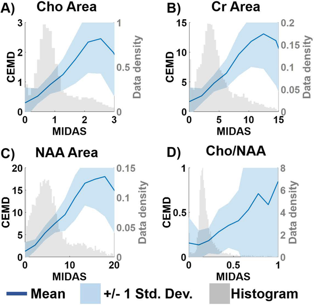
Correlations between the metabolite concentrations and the Cho/NAA ratio, calculated by CEMD and MIDAS for the testing set are shown in Figure 4. The solid blue lines plot the mean value between the two fitting techniques for each bin of values, and the shaded blue region indicates +/− 1 standard deviation. Overlaid in light gray are the histograms for the distribution of metabolite values computed by MIDAS. The variance of CEMD predictions compared to MIDAS is inversely correlated with the number of training samples available. While the two algorithms are linear in the regions where most of the data are present, CEMD has greater uncertainty at the tail end of the histograms where there were fewer training data.
Figure 4.
A comparison of the metabolite values and the Cho/NAA ratio computed by MIDAS and CEMD on the training set of spectra. The gray histogram shows the distribution of MIDAS calculations; the dark blue line indicates the mean values of CEMD and MIDAS in each histogram bin; the shaded blue region indicates the +/− 1 standard deviation of CEMD calculations.
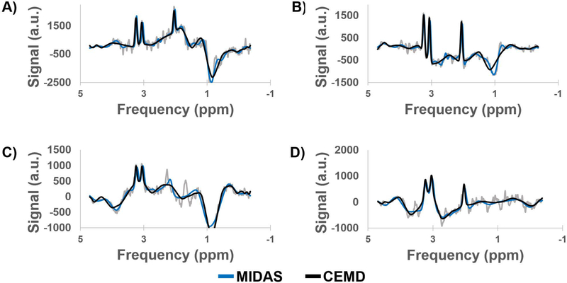
Figure 5 compares the fits by MIDAS (blue) and CEMD (black) for several challenging spectra from subjects with glioblastoma. The first (Figure 5A) depicts a spectrum with a large baseline shift on the right-side of the NAA peak. The second (Figure 5B) shows a spectrum with a large decline of the baseline on the Cho and Cr peaks but a flat baseline near the NAA peak. The third (Figure 5C) shows a spectrum from a voxel near the inferior rim of the surgical cavity, where partial volume effects reduce the apparent signal-to-noise ratio and where there is an absence of the NAA peak at 2.0 ppm. The fourth (Figure 5D) depicts a spectrum from the bone-cortex interface in the temporal; all peaks have broadened linewidth and the NAA peak is adjacent to large noise and lipid signal. All results show comparable performance for fitting of the metabolite peaks with some differences in the baselines.
Figure 5.
A comparison of the fits produced by MIDAS (blue) and CEMD (black) on several challenging spectra taken from patients with glioblastoma. a.u. = arbitrary units.
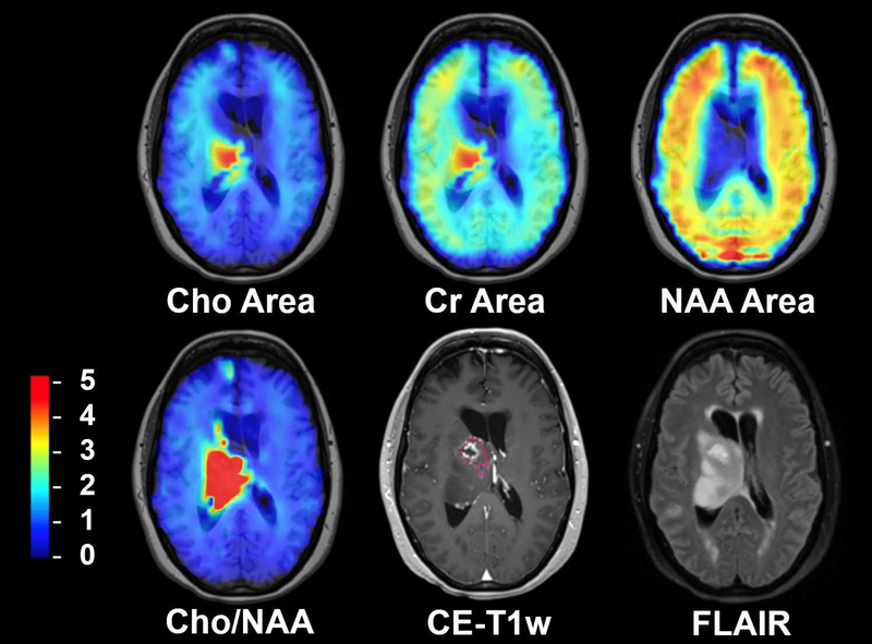
Results of the CEMD analysis for studies of a subject with glioblastoma, not included in the training set, are shown in Figure 6, which shows the individual metabolite maps, the Cho/NAA ratio map, and corresponding contrast-enhanced T1-weighted (CE-T1w) and fluid-attenuated inversion recovery (FLAIR) MRI volumes. Superimposed on the CE-T1w image is a contour drawn by a neuroradiologist to indicate contrast enhancing tissue and the surgical cavity, regions that would normally be targeted for high dose radiation therapy.
Figure 6.
An example of whole-brain metabolite maps generated by CEMD for a patient with a midline glioblastoma in comparison with standard imaging. The Cho/NAA volume indicates the presence of metabolically active tumor around the resection cavity extending beyond the contrast-enhancing lesion. Color bar corresponding to relative Cho/NAA values (compared to contralateral normal-appearing white matter) for Cho/NAA image; arbitrary units for metabolite maps. Pink contour indicated neuroradiologist-segmented contrast-enhancing tissue around the resection cavity.
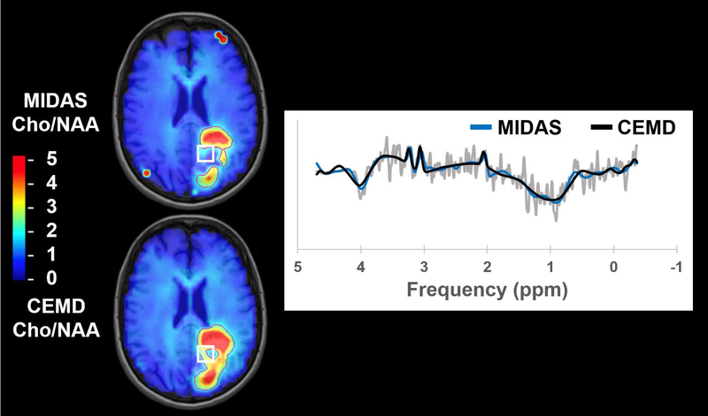
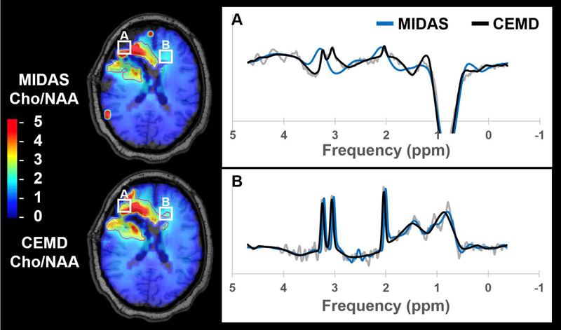
Cho/NAA abnormality volumes were contoured for CEMD and MIDAS fitting and the results are shown in Table 1, which includes subject-wise execution time, abnormality volumes, and DSC. The mean execution time for whole-brain spectral fitting was 20.6 +/− 2.8 sec using the CEMD. As a representative example, the execution time for CEMD on Subject 6 was broken down as follows: 2.7 seconds to load 11,702 spectra from disk into memory; 17.0 seconds to load the CEMD encoder model and to process all spectra; 3.3 seconds to create volumetric maps for each metabolite and the Cho/NAA ratio and to write these maps to disk. On average, CEMD-derived lesion volumes are larger by 1.2 cm3 (P = 0.83 using a two-tailed paired T test) and in several subjects encapsulated the contours produced from the MIDAS analysis. The mean DSC between CEMD and MIDAS was 0.72 +/− 0.13. In Figure 7 and Figure 8, Cho/NAA volumes computed by MIDAS and CEMD for Subjects 9 and 1, respectively, were qualitatively compared; the contours indicate a twofold increase in Cho/NAA compared to contralateral white matter. Isolated bright spots are artifacts due to fitting errors and were not contoured. A spectrum from an area where the two algorithms had different values of Cho/NAA (white box) is shown for each subject, with CEMD fit (black) and MIDAS fit (blue) overlaid on the spectrum (gray). Discrepancies occur either due to the calculated ratio being just above or below the 2x threshold (Figure 8B), or in areas of minimal or poor signal quality and therefore the uncertainties in the measurements must be considered to be very high.
Table 1.
Subject-wise comparison of the execution times for CEMD and the twice elevated Cho/NAA volumes generated by CEMD and MIDAS.
| Subject | CEMD Time (sec) | 2x Cho/NAA Vol. (cm3) | Volume Difference (cm3) | DSC | Z Test P Value | |
|---|---|---|---|---|---|---|
| CEMD | MIDAS | |||||
| 1 | 17.8 | 57.9 | 56.7 | 1.2 | 0.84 | 0.047 |
| 2 | 26.3 | 31.9 | 35.1 | −3.2 | 0.56 | 0.410 |
| 3 | 18.1 | 72.2 | 76.0 | −3.8 | 0.87 | 0.026 |
| 4 | 21.0 | 35.9 | 39.9 | −4.1 | 0.65 | 0.265 |
| 5 | 17.4 | 23.0 | 39.6 | −16.7 | 0.64 | 0.277 |
| 6 | 23.0 | 5.9 | 4.0 | 1.8 | 0.59 | 0.366 |
| 7 | 19.0 | 105.2 | 134.1 | −28.8 | 0.86 | 0.037 |
| 8 | 20.4 | 86.9 | 60.0 | 26.9 | 0.75 | 0.141 |
| 9 | 20.1 | 54.9 | 22.8 | 32.1 | 0.57 | 0.385 |
| 10 | 23.1 | 37.7 | 30.7 | 7.0 | 0.81 | 0.072 |
| Mean | 20.6 | -- | -- | 1.2 | 0.72 | -- |
| Std. Dev | 2.8 | -- | -- | 18.1 | 0.13 | -- |
Figure 7.
A comparison of the Cho/NAA volumes generated by MIDAS and CEMD in a subject with glioblastoma. Contours indicate Cho/NAA values greater than two-fold the value in contralateral normal appearing white matter. The spectrum shown comes from the highlighted voxel (white box).
Figure 8.
A comparison of Cho/NAA volumes generated by MIDAS (blue) and CEMD (black) in a second subject with glioblastoma, with spectra from the highlighted voxels (white boxes) shown. Contours indicate the isoline for Cho/NAA values greater than two-fold the value in contralateral normal appearing white matter.
Discussion
In recent years, machine learning has seen tremendous advances and has shattered benchmarks in a variety of fields, including medical imaging applications (38). While these deep learning approaches, including CNNs, can outperform less complex models, a key issue is that of interpretability. Several techniques, such as gradient-weighted class activation mapping (43), seek to elucidate some of the internal workings of CNNs and provide insight as to why the CNN predicted a particular output. Even so, this is always done in a retrospective fashion after the CNN has already been trained, and thus insights cannot be used to modify the algorithm. It is difficult to incorporate a priori domain knowledge into deep learning because these techniques are fundamentally data-driven rather than model or knowledge driven. However, recent work has suggested that the incorporation of domain knowledge may be able to improve the performance of deep learning models (44,45).
In this work, a deep learning approach to spectral fitting that incorporates a priori spectral information was developed and evaluated. Spectral fitting is the computational bottleneck in processing of volumetric MRSI, largely because the existing methods are based on iterative algorithms. The CEMD is an unsupervised deep learning architecture that incorporates spectral models to generate an encoding of spectral parameters, which is advantageous because it does not require any “ground truth” spectral quantitation for training. The predictions of the CEMD have contextual meaning, and the CEMD was trained to make these predictions within the constraints of an explicitly defined spectral model. Once trained, the CEMD performs spectral fitting on volumetric data in under one minute using standard computer hardware. The order of magnitude improvement in fitting time can greatly benefit the clinical adoption of whole-brain MRSI. This architecture could be implemented on scanner computers, enabling real-time reconstruction and review of data without the need for offloading of data to more specialized computer systems. Fitted data and metabolite volumes could then easily be sent to a clinical PACS systems in a streamlined fashion.
Incorporation of knowledge of the spectral model imposes constraints that are important for the assessment of spectra. Bhat et. al. previously incorporated spectral models in an unsupervised neural network; however, their model was limited in requiring baseline-corrected spectra as input to their neural network (27). CEMD simultaneously computes the baseline and peak components of the spectrum and correctly identifies singlets in challenging spectra such as those in Figure 5. The spectrum in Figure 5C indicates the loss of the NAA resonance at 2.0 ppm. It is necessary for a fitting model understand where the NAA resonance should be and not attempt to model other peak-like shapes (e.g. at 2.3 ppm and 1.7 ppm) as NAA. For spectra where asymmetric broadening of peaks occurs, the spectral lineshape model dictates that a symmetric peak should be fit (Figure 5D). In these cases, CEMD performed on par with traditional parametric analysis algorithms such as that incorporated in MIDAS.
For this study only the real part of the complex spectral data was used as input for CEMD and in the cost function for updating the CNN weights, though a complex spectral model (Equation 4) was used in the decoder. We note that the phase correction terms were accurately reported. It is speculated that this occurs through an observation from the asymmetry of the lineshape (46). An initial implementation of CEMD using the full complex spectral data found reduced performance (mean fit RMSE of 38%), potentially due to the increased number of parameters in the encoder that would need to be trained.
While the CEMD was trained using data obtained on a single 3T scanner, this study has demonstrated generalizability to data acquired on other instruments using the same acquisition parameters (Figure 3); however, this study has not evaluated the extension to other pulse sequence parameters. If studies are to be performed using different acquisition schemes, such as with shorter TE, CEMD would have to be retrained. However, training does not require many subjects because of the ~10,000 spectra in each study. The CEMD could be adapted, e.g. changing the number and type of layers in the encoder and number of coefficients in the decoder models, for more resonances, of multiplets of resonances, or of metabolites whose resonance peaks are not readily separable (gluatamate and glutamine). In general, because the autoencoder scheme does not rely on any external “ground truth” data, it can be readily adapted and optimized for different complexities of fitting.
In this work, a comparison between this new fitting paradigm and an existing iterative parametric optimization method was performed. The results in Figure 4 show the correlation between the two algorithms’ estimation of Cho, Cr, and NAA resonances and the Cho/NAA ratio on the same set of spectra. In spectroscopy, the acquired spectral signal amplitude is uncalibrated, and additional methods are required to apply a signal normalization procedure. Ratios, such as Cho/NAA, do not require calibration; however, they are more unstable when the denominator is low. As seen in Figure 4D, both CEMD and MIDAS fitting have high uncertainty for high Cho/NAA values that represent low NAA regions. While individual metabolite resonance maps are shown in Figure 6 to assess the ability of CEMD to perform whole-brain fitting, the Cho/NAA maps are used as the main comparison between CEMD and an existing parametric analysis (MIDAS) in Table 1. CEMD achieves a Dice coefficient of 0.72 when compared to MIDAS. A key observation is that CEMD can produce similar Cho/NAA volumes to MIDAS while never being trained to do so; thus, it independently achieves similar results, which highlights the power of unsupervised learning techniques.
Qualitatively, as seen in Figures 7 and 8, CEMD produces similar spatial distributions of the Cho/NAA ratio as MIDAS in subjects with glioblastoma. Both algorithms identify the region of brain with an elevated ratio, though occasionally with different contour shape and size when selecting voxels with a Cho/NAA abnormality greater than 2x contralateral NAWM (Table 1). These differences hold when adjusting this threshold on two sample cases, one from a subject with high DSC conformality and another with low DSC conformality (Supporting Information Table S1). The study for Subject 9 has poor DSC; reviewing spectra in which the two fitting algorithms produced different values of Cho/NAA reveals that these discordant fits occur in regions of low spectral SNR surrounding the rim of the surgical cavity. Two possible reasons underlying this discordance are speculated. The first is highlighted in Figure 7, in which CEMD estimates a slightly lower value for the NAA resonance peak compared to MIDAS, and therefore estimates a Cho/NAA above the 2x threshold. A similar discrepancy in the Cho/NAA value can be observed in Subject 1 in the contralateral extension of the CEMD contour in Figure 8B. While using a threshold of a twofold increase in Cho/NAA compared to NAWM has been previously established to identify a high probability of tumor, a voxel having a value just below the threshold does not mean the voxel is tumor-free. Ultimately, when using MRSI for therapeutic guidance or diagnosis, clinician insight is needed.
A second reason for discordance between the two algorithms is apparent in a voxel from Subject 1, shown in Figure 8A. CEMD has a tendency to overfit spectra with low SNR that occur near tissue interfaces, where magnetic field inhomogeneities and partial volume effects can cause large distortions. The highlighted voxel is deemed to be artifactual and should in fact have been removed. In general, results corresponding to low SNR data, as shown in Figures 7 and 8, can be excluded by post-processing that takes into account the uncertainty of the fit via metrics such as Cramér-Rao lower bounds (13,47). This is especially important when calculating metabolite ratios. One limitation of the current implementation of the CEMD fitting is that it does not include an estimate of the uncertainties of the fit and this needs to be further investigated, although our previously-described artifact filter may also be used for this purpose (23). While CEMD was built for spectral fitting for rapid turnaround time, for research purposes in which a more thorough analysis of spectral quantitation is desired, existing software such as MIDAS can be used.
Conclusion
In this work, a machine learning approach to spectral fitting is described that can perform sub-minute calculation of relative metabolite concentrations in MRSI of the brain. A convolutional encoder-model decoder technique has been implemented that explicitly incorporates a standard parametric spectral model with the power of unsupervised feature-learning to produce fast spectral fittings that are constrained by the standard model. This is a powerful paradigm that does not require a priori ground truth and relies upon previously-used spectral lineshape and baseline models to optimize the underlying convolutional neural network parameters. The CEMD architecture is shown to produce accurate fitting of a variety of spectra acquired from multiple scanners in patients with glioblastoma, including correctly fitting challenging spectra with low SNR, partial volume effects, baseline shifts, phase shifts, and dropout of one or more metabolite resonances. The CEMD can fit whole-brain data on a standard multicore computer without the need for expensive workstations or GPUs, in less than one minute. With this new autoencoder-based neural network, the largest computational bottleneck in processing MRSI can be overcome, bringing improved performance that will support the implementation of MRS for more widespread clinical use.
Supplementary Material
Supporting Information Figure S1. Detailed schematic of the CEMD architecture. CEMD features two serial encoder-decoder steps, the first which computes the baseline, and the second which fits resonance peaks on the baseline-subtracted spectrum. FC = fully connected.
Acknowledgements
The authors would like to thank the following individuals for their support in data collection: Peter B. Barker, Michal Povazan, Michael K. Larche, Robert L. Smith III, Samira Yeboah, Sarah Basadre, Pooya Mobadersany, and Mohamed Amgad. This work was supported by National Institutes of Health grants: U01 EB028145, R01 CA214557, R01 EB016064, and F30 CA206291.
References
- 1.Law M, Cha S, Knopp EA, Johnson G, Arnett J, Litt AW. High-grade gliomas and solitary metastases: differentiation by using perfusion and proton spectroscopic MR imaging. Radiology 2002;222(3):715–721. [DOI] [PubMed] [Google Scholar]
- 2.Soares DP, Law M. Magnetic resonance spectroscopy of the brain: review of metabolites and clinical applications. Clin Radiol 2009;64(1):12–21. [DOI] [PubMed] [Google Scholar]
- 3.Cordova JS, Shu H-KG, Liang Z, Gurbani SS, Cooper LAD, Holder CA, Olson JJ, Kairdolf B, Schreibmann E, Neill SG, Hadjipanayis CG, Shim H. Whole-brain spectroscopic MRI biomarkers identify infiltrating margins in glioblastoma patients. Neuro Oncol 2016;18(8):1180–1189. [DOI] [PMC free article] [PubMed] [Google Scholar]
- 4.Stadlbauer A, Buchfelder M, Doelken MT, Hammen T, Ganslandt O. Magnetic resonance spectroscopic imaging for visualization of the infiltration zone of glioma. Central European Neurosurgery 2011;72(02):63–69. [DOI] [PubMed] [Google Scholar]
- 5.Chronaiou I, Stensjøen AL, Sjøbakk TE, Esmaeili M, Bathen TF. Impacts of MR spectroscopic imaging on glioma patient management. Acta Oncologica 2014;53(5):580–589. [DOI] [PubMed] [Google Scholar]
- 6.Ken S, Vieillevigne L, Franceries X, Simon L, Supper C, Lotterie J-A, Filleron T, Lubrano V, Berry I, Cassol E. Integration method of 3D MR spectroscopy into treatment planning system for glioblastoma IMRT dose painting with integrated simultaneous boost. Radiation Oncology 2013;8(1):1. [DOI] [PMC free article] [PubMed] [Google Scholar]
- 7.Nelson SJ, Graves E, Pirzkall A, Li X, Antiniw Chan A, Vigneron DB, McKnight TR. In vivo molecular imaging for planning radiation therapy of gliomas: an application of 1H MRSI. Journal of Magnetic Resonance Imaging: An Official Journal of the International Society for Magnetic Resonance in Medicine 2002;16(4):464–476. [DOI] [PubMed] [Google Scholar]
- 8.Pirzkall A, McKnight TR, Graves EE, Carol MP, Sneed PK, Wara WW, Nelson SJ, Verhey LJ, Larson DA. MR-spectroscopy guided target delineation for high-grade gliomas. International Journal of Radiation Oncology* Biology* Physics 2001;50(4):915–928. [DOI] [PubMed] [Google Scholar]
- 9.Cordova JS, Kandula S, Gurbani S, Zhong J, Tejani M, Kayode O, Patel K, Prabhu R, Schreibmann E, Crocker I, Holder CA, Shim H, Shu H-K. Simulating the Effect of Spectroscopic MRI as a Metric for Radiation Therapy Planning in Patients with Glioblastoma. Tomography : a journal for imaging research 2016;2(4):366–373. [DOI] [PMC free article] [PubMed] [Google Scholar]
- 10.Gurbani S, Mellon E, Weinberg B, Schreibmann E, Maudsley AA, Sheriff S, Barker PB, Kleinberg L, Cooper LAD, Shu H-K, Shim H. A Feasibility Study of Radiation Therapy Dose Escalation Guided by Spectroscopic Magnetic Resonance Imaging in Patients with Glioblastoma. 2018; Paris, FR: p Abstract #1155. [Google Scholar]
- 11.Mierisová Š, Ala‐Korpela M. MR spectroscopy quantitation: a review of frequency domain methods. NMR in Biomedicine: An International Journal Devoted to the Development and Application of Magnetic Resonance In Vivo 2001;14(4):247–259. [DOI] [PubMed] [Google Scholar]
- 12.Vanhamme L, Sundin T, Hecke PV, Huffel SV. MR spectroscopy quantitation: a review of time‐domain methods. NMR in Biomedicine: An International Journal Devoted to the Development and Application of Magnetic Resonance In Vivo 2001;14(4):233–246. [DOI] [PubMed] [Google Scholar]
- 13.Provencher SW. Automatic quantitation of localized in vivo1H spectra with LCModel. NMR Biomed 2001;14(4):260–264. [DOI] [PubMed] [Google Scholar]
- 14.Young K, Soher BJ, Maudsley AA. Automated spectral analysis II: application of wavelet shrinkage for characterization of non-parameterized signals. Magn Reson Med 1998;40(6):816–821. [DOI] [PubMed] [Google Scholar]
- 15.Soher BJ, Young K, Govindaraju V, Maudsley AA. Automated spectral analysis III: application to in vivo proton MR spectroscopy and spectroscopic imaging. Magn Reson Med 1998;40(6):822–831. [DOI] [PubMed] [Google Scholar]
- 16.Stefan D, Di Cesare F, Andrasescu A, Popa E, Lazariev A, Vescovo E, Strbak O, Williams S, Starcuk Z, Cabanas M. Quantitation of magnetic resonance spectroscopy signals: the jMRUI software package. Measurement Science and Technology 2009;20(10):104035. [Google Scholar]
- 17.Wilson M, Reynolds G, Kauppinen RA, Arvanitis TN, Peet AC. A constrained least-squares approach to the automated quantitation of in vivo 1H magnetic resonance spectroscopy data. Magnetic Resonance in Medicine 2010;65(1):1–12. [DOI] [PubMed] [Google Scholar]
- 18.Lam F, Liang ZP. A subspace approach to high‐resolution spectroscopic imaging. Magnetic resonance in medicine 2014;71(4):1349–1357. [DOI] [PMC free article] [PubMed] [Google Scholar]
- 19.Reynolds G, Wilson M, Peet A, Arvanitis TN. An algorithm for the automated quantitation of metabolites in in vitro NMR signals. Magnetic Resonance in Medicine 2006;56(6):1211–1219. [DOI] [PubMed] [Google Scholar]
- 20.Maudsley AA, Domenig C, Govind V, Darkazanli A, Studholme C, Arheart K, Bloomer C. Mapping of brain metabolite distributions by volumetric proton MR spectroscopic imaging (MRSI). Magn Reson Med 2009;61(3):548–559. [DOI] [PMC free article] [PubMed] [Google Scholar]
- 21.Sabati M, Sheriff S, Gu M, Wei J, Zhu H, Barker PB, Spielman DM, Alger JR, Maudsley AA. Multivendor implementation and comparison of volumetric whole-brain echo-planar MR spectroscopic imaging. Magn Reson Med 2015;74(5):1209–1220. [DOI] [PMC free article] [PubMed] [Google Scholar]
- 22.Kyathanahally SP, Mocioiu V, Pedrosa de Barros N, Slotboom J, Wright AJ, Julià‐Sapé M, Arús C, Kreis R. Quality of clinical brain tumor MR spectra judged by humans and machine learning tools. Magnetic resonance in medicine 2018;79(5):2500–2510. [DOI] [PubMed] [Google Scholar]
- 23.Gurbani SS, Schreibmann E, Maudsley AA, Cordova JS, Soher BJ, Poptani H, Verma G, Barker PB, Shim H, Cooper LAD. A convolutional neural network to filter artifacts in spectroscopic MRI. Magnetic Resonance in Medicine 2018;80(5):1765–1775. [DOI] [PMC free article] [PubMed] [Google Scholar]
- 24.Pedrosa de Barros N, McKinley R, Knecht U, Wiest R, Slotboom J. Automatic quality control in clinical (1)H MRSI of brain cancer. NMR Biomed 2016;29(5):563–575. [DOI] [PubMed] [Google Scholar]
- 25.Pedrosa de Barros N, McKinley R, Wiest R, Slotboom J. Improving labeling efficiency in automatic quality control of MRSI data. Magn Reson Med 2017. [DOI] [PubMed] [Google Scholar]
- 26.Hiltunen Y, Kaartinen J, Pulkkinen J, Häkkinen A-M, Lundbom N, Kauppinen RA. Quantification of Human Brain Metabolites from in Vivo1H NMR Magnitude Spectra Using Automated Artificial Neural Network Analysis. Journal of Magnetic Resonance 2002;154(1):1–5. [DOI] [PubMed] [Google Scholar]
- 27.Bhat H, Sajja BR, Narayana PA. Fast quantification of proton magnetic resonance spectroscopic imaging with artificial neural networks. Journal of Magnetic Resonance 2006;183(1):110–122. [DOI] [PMC free article] [PubMed] [Google Scholar]
- 28.Das D, Coello E, Sekuboyina A, Schulte RF, Menze BH. Direct Estimation of Model Parameters in MR Spectroscopic Imaging using Deep Neural Networks. 2018; Paris, FR: p Abstract #3852. [Google Scholar]
- 29.Liou C-Y, Huang J-C, Yang W-C. Modeling word perception using the Elman network. Neurocomputing 2008;71(16):3150–3157. [Google Scholar]
- 30.Hinton GE, Salakhutdinov RR. Reducing the dimensionality of data with neural networks. Science 2006;313(5786):504–507. [DOI] [PubMed] [Google Scholar]
- 31.Griswold MA, Jakob PM, Heidemann RM, Nittka M, Jellus V, Wang J, Kiefer B, Haase A. Generalized autocalibrating partially parallel acquisitions (GRAPPA). Magnetic Resonance in Medicine: An Official Journal of the International Society for Magnetic Resonance in Medicine 2002;47(6):1202–1210. [DOI] [PubMed] [Google Scholar]
- 32.Goodfellow I, Bengio Y, Courville A. Deep Learning: MIT Press; 2016. 800 p. [Google Scholar]
- 33.Wei Dai CDSQJLSD. Very Deep Convolutional Neural Networks for Raw Waveforms. 2016.
- 34.Donoho DL, Johnstone IM. Adapting to Unknown Smoothness via Wavelet Shrinkage. J Am Stat Assoc 1995;90(432):1200–1224. [Google Scholar]
- 35.Daubechies I Ten lectures on wavelets: Siam; 1992.
- 36.Abadi M, Barham P, Chen J, Chen Z, Davis A, Dean J, Devin M, Ghemawat S, Irving G, Isard M. Tensorflow: a system for large-scale machine learning. 2016. p 265–283.
- 37.Strang G, Nguyen T. Wavelets and filter banks: SIAM; 1996.
- 38.LeCun Y, Bengio Y, Hinton G. Deep learning. Nature 2015;521(7553):436–444. [DOI] [PubMed] [Google Scholar]
- 39.Kingma DP, Ba J. Adam: A Method for Stochastic Optimization. 3rd International Conference for Learning Representaitons San Diego, CA, USA2015. [Google Scholar]
- 40.Gurbani SS, Schreibmann E, Sheriff S, Holder CA, Cooper LAD, Maudsley A, Shim H. Rapid Internal Normalization of Spectroscopic MRI Maps Using a Gaussian Mixture Model. 2017; Denver, CO. p TU-AB-601–610. [Google Scholar]
- 41.Dice LR. Measures of the amount of ecologic association between species. Ecology 1945;26(3):297–302. [Google Scholar]
- 42.Zou KH, Warfield SK, Bharatha A, Tempany CMC, Kaus MR, Haker SJ, Wells WM, Jolesz FA, Kikinis R. Statistical Validation of Image Segmentation Quality Based on a Spatial Overlap Index: Scientific Reports. Academic radiology 2004;11(2):178–189. [DOI] [PMC free article] [PubMed] [Google Scholar]
- 43.Selaraju R, Das A, Vedantam R, Cogswell M, Parikh D, Batra D. Grad-CAM: Why did you say that? Visual Explanations from Deep Networks via Gradient-based Localization. CoRR 2016;abs/1610.02391. [Google Scholar]
- 44.Vo K, Pham D, Nguyen M, Mai T, Quan T. Combination of Domain Knowledge and Deep Learning for Sentiment Analysis. 2017. Springer; p 162–173. [Google Scholar]
- 45.Yu T, Jan T, Simoff S, Debenham J. Incorporating prior domain knowledge into inductive machine learning.
- 46.Heuer A A new algorithm for automatic phase correction by symmetrizing lines. Journal of Magnetic Resonance (1969) 1991;91(2):241–253. [Google Scholar]
- 47.Jiru F, Skoch A, Klose U, Grodd W, Hajek M. Error images for spectroscopic imaging by LCModel using Cramer-Rao bounds. MAGMA 2006;19(1):1–14. [DOI] [PubMed] [Google Scholar]
Associated Data
This section collects any data citations, data availability statements, or supplementary materials included in this article.
Supplementary Materials
Supporting Information Figure S1. Detailed schematic of the CEMD architecture. CEMD features two serial encoder-decoder steps, the first which computes the baseline, and the second which fits resonance peaks on the baseline-subtracted spectrum. FC = fully connected.


