Abstract
Brain-machine interfaces (BMIs) have been widely used to study basic and translational neuro-science questions. In real-time closed-loop neuroscience experiments, many practical issues arise, such as trial-by-trial variability, and spike sorting noise or multi-unit activity. In this paper, we propose a new framework for change-point detection based on ensembles of independent detectors in the context of BMI application for detecting acute pain signals. Motivated from ensemble learning, our proposed “ensembles of change-point detectors” (ECPDs) integrate multiple decisions from independent detectors, which may be derived based on data recorded from different trials, data recorded from different brain regions, data of different modalities, or models derived from different learning methods. By integrating multiple sources of information, the ECPDs aim to improve detection accuracy (in terms of true positive and true negative rates) and achieve an optimal trade-off of sensitivity and specificity. We validate our method using computer simulations and experimental recordings from freely behaving rats. Our results have shown superior and robust performance of ECPDS in detecting the onset of acute pain signals based on neuronal population spike activity (or combined with local field potentials) recorded from single or multiple brain regions.
Keywords: Brain machine interface, Change point detection, Ensemble learning, Population codes, Acute Pain, Poisson linear dynamical system, Support vector machine, Event-related potential
1. Introduction
An important problem in closed-loop neuroscience experiments is to quickly identify abrupt changes in neural ensemble spike activity induced by external stimuli or internal change in brain states. Although the univariate or multivariate change-point detection problem has been widely studied, most of studies have been limited to continuous or discrete time series with assumed probability distributions (Aminikhanghahi & Cook 2017, Xie et al. 2013, Kopepcke et al. 2016, Pillow et al. 2011). In neuroscience experiments, changes are reflected in the neuronal ensemble spike activity and local field potential (LFP), which may directly relate to the change in behavior or attention. In real-time closed-loop brain-machine interface (BMI) applications, the challenge is how to design online detection algorithms that can quickly and reliably detect these changes (Hu et al. 2017). Previously, we have designed and tested several algorithms in an off-line setting (Chen et al. 2017a, Chen et al. 2017b). However, for online BMI applications, we need to consider several important issues: first, the limited sample size for training a complex model; second, the nonstationarity of data induced by the irregular animal behavior; third, the spike sorting noise and multiu-nit activity that affect the overall signal-to-noise ratio (SNR) (Goodman & Johnson 2008, Fraser et al. 2009); and fourth, the mixed selectivity of neuronal tuning. The first issue involves non-global optimization in model estimation, especially in the presence of a large number of neurons and shorter recording duration. In this paper, we aim to address the remaining three issues in the application of detecting pain signals from neuronal ensemble spike activity.
Pain is a common experience in life, but pain mechanisms in the brain remain poorly understood. In patients, pain remains defined by verbal reports. The challenge is to identify the most relevant brain areas or neural ensembles underlying pain behavior. Identification of such neural ensembles could effectively provide a “neural code” for pain. A number of human neuroimaging studies identify several brain regions that respond to pain stimuli, including the anterior cingulate cortex (ACC) and primary somatosensory cortex (S1) (Vogt 2005, Perl 2007, Bushnell et al. 2013, Vierck et al. 2013). Neurophysiological recordings of ACC and S1 from rodent experiments also confirm these findings (Kuo & Yen 2005, Zhang et al. 2011, Chen et al. 2017a, Zhang et al. 2017). Detection of pain signals from neural recordings has direct clinical applications. First, it can be used for assessment of anesthetic drugs for pain management. Second, it can be used for pain treatment. This demand-based pain neuromodulation de-pends critically on timely identification of the pain sig-nal and ultrafast neuromodulation. Optogenetic stim-ulations have provided an effective way for neuromoduation in rodent experiments (Daou et al. 2013, Lee et al. 2015, Gu et al. 2015, Iyer et al. 2016, Copits et al. 2016). Importantly, a BMI for achieving closed-loop pain control requires timely and precise detection of pain signals. This has motivated us to use animal models to study the pathophysiology of pain (Xu & Brennan 2011, Zhang et al. 2017).
Ensemble learning, in either supervised or unsupervised form, is an active research topic in machine learning (Kittler et al. 1998, Liu & Yao 1999, Dietterich 2000, Kuncheva 2004, Raykar et al. 2010). In short, ensemble learning is aimed to combine a set of possibly “weak” learners (predictors, classifiers, detectors, etc.) to form a more accurate “meta learner” in decision making. In unsupervised ensemble learning, the decision is made without the labeled data (Parisi et al. 2014, Jaffe et al. 2015). To date, unsupervised learning methods have not been widely adopted in BMI applications. Unlike supervised learning methods, unsupervised learning methods do not required many labeled examples for training, and thus are less prone to overfitting. In our current application of interest, it is worthy emphasizing several key differences from the standard methods in the literature. First, in ensembles of unsupervised classifiers, the samples are independent, identically distributed (i.i.d.); whereas the samples in our application are temporal correlated multivariate time series. Second, in traditional ensemble learning, the predictors or classifiers are often derived from different models; whereas in our application, the detectors may be drawn from the same model family. Third, a new consensus decision rule can be derived based on the detection results derived from two simultaneously recorded brain regions.
The detection performance in BMI applications is assessed by detection latency and accuracy. While the issue of detection speed has been treated elsewhere (Hu et al. 2018), here we focus our investigation on detection accuracy (sensitivity and specificity), indicated by false positive (FP) and false negative (FN) rates. In the context of detecting pain signals, a great challenge arises when neurons show mixed tuning selectivity in response to pain (noxious) stimuli and non-pain (non-noxious) stimuli. Therefore, we aim to design a robust and reliable strategy to detect pain signals under various experimental conditions.
To meet this research goal, we propose a generic ensemble detection framework for detecting acute pain signals. Specifically, a set of independent “weak” change-point detectors are constructed from independent ob-servations or trials, from which we construct a meta detector with custom decision rules to improve detection accuracy. The individual change-point detectors are derived from either unsupervised or supervised learning. We validate our method using computer simulations and in vivo experimental recordings from freely behav-ing rats. Through computer simulations, we systematically investigate the impact of cell specificity, mixed selectivity of neuronal tuning, SNR, and trial-by-trial variability on the performance of ensembles of change-point detectors (ECPDs). In an experimental investigation for detecting acute pain signals, our contribution includes three aspects of innovations: (i) integrating multiple models trained by preceding trials; (ii) integrating multiple brain regions from S1 and ACC population spikes, using either single or multiple models; and (iii) integrating information from ensemble spikes and LFP based on multiple brain regions.
2. Materials and Methods
2.1. Animal Behavior and Physiological Recordings
All experimental studies were performed in accordance with the New York University School of Medicine (NYU-SOM) Institutional Animal Care and Use Committee and the National Institutes of Health (NIH) Guide for the Care and Use of Laboratory Animals to ensure minimal animal use and discomfort. Male Sprague-Dawley rats were used in all experiments. Several types of noxious and non-noxious stimuli were used in our investigations. One type of acute thermal pain stimulus was delivered by a blue (473 nm diode-pumped solid-state) laser with varying laser intensities (50–250 mW) (Chen et al. 2017a, Zhang et al. 2017). Another type of acute mechanical pain stimulus was a pin prick. The intertrial intervals between consecutive laser stimulations varied between 1 to 2 minutes.
Animals freely explored in a plastic chamber of size 38 × 20 × 25 cm3. One video camera (120 frame per second) was used to continuously record the animal behavior. A common characterization of an animal’s pain behavior is its latency to paw withdrawal, and the duration of paw licking (Cheppudira 2006). We con-structed custom tetrode or stereotrode arrays, or used bundled silicon probes to record neural activity from the rat ACC or S1 areas, or simultaneously from both regions. Using a Plexon (Dallas, TX) data acquisition system, the spikes were thresholded from high-passed (>300 Hz) local field potentials. Similar to the real-time BMI setup, the spikes were further sorted online based on spike waveform features such as peak amplitude, energy, and principal components. We used all sorted units, including all putative pyramidal neurons and interneurons, in our subsequent analysis. According to the unit response property, we define three classes of units: Class 1 consists of pain-modulated units, Class 2 consist of non-pain-modulated units, and Class 3 consists of non-response units. In our empirical observations (Chen et al. 2017a), the proportion of Class 1 units varies in each recording session (15–20%).
The experimental recordings from 3 rats selected for our current study are summarized in Table 1. The 50 mW laser stimulation and van Frey are negative controls (for assessing FP), whereas 150 or 250 mW laser stimulation and pin prick are positive controls (for assessing TP).
Table 1.
Summary of experimental recording sessions. Two numbers in the 4th column are referred to the numbers of trials associated with simulation of two laser intensities or two stimuli, respectively.
| Session | Region | Pain stimulus | # trials | # units | Electrode |
|---|---|---|---|---|---|
| 1 | ACC | 50/150 mW laser | 25/25 | 32 | stereotrode (32 channels) |
| 2 | ACC | 50/150 mW laser | 25/25 | 34 | stereotrode (32 channels) |
| 3 | S1 | 50/250 mW laser | 30/30 | 43 | silicon probe (32 channels) |
| 4 | S1 | 50/250 mW laser | 30/30 | 36 | silicon probe (32 channels) |
| 5 | ACC+S1 | 50/250 mW laser | 18/19 | 10+7 | tetrode (32 channels) |
| 6 | ACC+S1 | pin prick/von-frey | 20/24 | 12+9 | tetrode (32 channels) |
| 7 | ACC+S1 | 50/250 mW laser | 20/20 | 28+24 | silicon probe (64 channels) |
2.2. Model-based Method for Change-point Detection
Our model-based method for change-point detection is based on state space analysis (Chen 2015, Chen et al. 2017a). Let yk = [y1,k, . . . , yC,k]⊤ denote a C-dimensional population vector, with each element consisting of the neuronal spike count within the k-th time bin or the interval [(k−1)Δ, kΔ) (where is the temporal bin size). The latent univariate variable zk ∈ ℝ represents an un-observed common input that drives neuronal ensemble spiking activity.
2.2.1. Poisson linear dynamical system
Pain is an abstract and emotional experience, and thus pain signals are hidden and evolve dynamically in time. We consider a latent variable model known as Poisson linear dynamical system (PLDS) to link the pain stimulus to neural activity (Chen et al. 2017a), where the spike activity of a population of C neurons are assumed to be drawn from the following generative model:
| (1) |
| (2) |
where the univariate (latent) variable zk represents the hidden common input that drives the neuronal population firing rate. The dynamics of the latent variable is governed by Eq. (1), which describes a first-order autoregressive (AR) model (0 < |a| < 1) driven by a zero-mean Gaussian noise process ∈k ∈ N (0, σ2∈). The parameters c and d are unconstrained. Based on maximum likelihood estimation, we use an expectation-maximization (EM) algorithm to estimate the unknown state variables z1:T and parameters Θ = {a, c, d, σ∈} from a set of observations y1:T. Details are referred to previously published materials (Macke et al. 2015, Chen et al. 2017a)
2.2.2. Online recursive filtering
In online BMI applications, once the model parameters are identified, we use a recursive (forward) filter to estimate the latent state variable (Chen et al. 2017a, Chen et al. 2017b):
| (3) |
| (4) |
| (5) |
| (6) |
| (7) |
where Qk|k = Var[ˆzk|k] denotes the filtered state variance. In our online filtering algorithm, we set the initial condition zˆ0|0 = 0 and Q0|0 from the pretrained model.
2.2.3. Criterion for change-point detection
The change of ensemble spike activity is defined with respect to a predefined baseline, which is often referred to as a short relatively stationary duration (e.g., 4–5 s) before the stimulus presentation. From the online estimate zˆk|k, we compute the Z-score with respect to the baseline: and convert it to probability (Chen & Wang 2016, Chen et al. 2017a):
| (8) |
The Z-score during the baseline is called Zbaseline. The criterion of Z-score change is determined by a statistical threshold θ0 depending on the significance level. When P= 0.05, θ0 = 1.65; when P = 0.01, θ0 = 2.33; when P= 0.001, θ0 = 3.08. Therefore, it is concluded that a change-point occurs when Z-score−CI > θ0 or Z-score+ change-point occurs when Z-score−CI > θ0 or Z-score+ CI < −θ0, where the CI denotes the confidence interval derived from the posterior variance of .The algebraic sign of the Z-score is irrelevant due to the sign ambiguity of in model estimation.
Therefore, the estimated PLDS model defines a single model-based detector for change points. Unless specified otherwise, we use P < 0.05 as the significance criterion.
2.3. Ensembles of Change-point Detectors
In our application, the above-described PLDS model defines a single detector for change points. Given N independent detectors, at any moment, from Eq. (8) we can derive a probability of significance change from each detector. In general, assume that the j-th detector produces a probability of change at time k: P(ωj,k|y0:k) with a prior probability Pj, then based on the “product rule”, the joint decision rule for ωk ∈{0,1} (1 denotes a change and 0 no change) can be formulated mathematically as follows:
| (9) |
In the case of using non-informative priors, Pj is set to be equal among N detectors.
Alternatively, we can use ensemble averaging of independent models based on the “sum rule”:
| (10) |
where {αj } denotes a set of weights associated with each expert. The joint decision is constructed by a lin-ear combination of experts. Identification of the weights can be achieved by supervised learning using labeled data. However, when the labeled data are limited, this approach is impractical in BMI applications.
Similar to classification (Kittler et al. 1998), we may design different decision rules for detection, such as the greedy rule and majority vote rule. The greedy rule claims a change point as long as one detector predicts the change. The majority vote rule states the class ωk = 0/1 that receives the largest number of votes is selected as the consensus or majority vote, assuming equal prior probabilities. Such a group decision based on the ensembles of change-point detectors (ECPDs) is known as the committee decision.
In our experimental context, we have a set of in-dependent model detectors. By using a majority vote rule, we expect to improve the robustness and accuracy of change-point detection.
2.4. Combining Two Brain Regions
Among many brain regions, the S1 and ACC are two of the most studied areas for nociceptive and pain perception (Kuo & Yen 2005, Vogt 2005, Bushnell et al. 2013). The S1 encodes the sensory component of pain, whereas the ACC encodes the aversive component of pain. However, neither of these areas is pain-specific; they may encode other sensory or emotional responses to non-noxious (somatosensory or sensory) stimuli (Urien et al. 2018). In our preliminary investigations, we found that S1 and ACC populations have different degrees of sensitivity and specificity for encoding pain stimuli (Chen et al. 2017a). In general, S1 tends to have high sensitivity for noxious stimuli, but it can also cause false alarms for non-noxious stimuli. On the other hand, ACC tends to have mixed selectivity or conjunctive coding for a va-riety of stimuli related to emotion, nociception and anticipation. Therefore, it is important to design specific rules for detecting acute pain based on their response properties. The optimality of the rule may depend on the experiment and specific simultaneously recorded S1 and ACC ensemble spike activities.
In addition to Eqs. (9) and (10), we consider an unsupervised learning method without labeled data. Specifically, we employ a decision rule based on a time-varying cross-correlation function (CCF) between the Z-scores Zk from two brain regions
| (11) |
where 0 < ρ < 1 is a forgetting factor, 0.5 ≤ m, n ≤ 1 are the scaling exponents (default value: 0.5). The smaller the forgetting factor ρ, the smoother the CCF curve. The purpose of scaling exponent is to control the impact of high/low Z-score values. For instance, a smaller exponent will magnify the impact of Z-score smaller than 1, while reducing the impact of a higher Z-score. Equation (11) assumes that when two Z-score traces follow a consistent trend, the CCF will increase in absolute value, and otherwise will stay at the baseline level. Since the Z-score estimate has uncertainty, we use the lower or upper bound of Zk—the choice depends on the algebraic sign: we use its lower bound for a positive Zk and use its upper bound for a negative Zk.
Similarly, we can compute the Z-score of CCF relative to the same baseline. We also track the CCF area above the threefold SD of baseline statistics. The area value will accumulate as long as the CCF is above the threshold, and will reset to 0 when the CCF is below the threshold. When the accumulated area value exceeds a predefined threshold θ, we declare the change point. The choice of θ depends on m, n and ρ. As expected, changing the threshold will affect the sensitivity and specificity of detection accuracy.
2.5. Size of Buffering Window
In online ensemble detection, a practical issue is how long we need to wait between different detection de-cisions? For an ensemble of N detectors, assuming the first moment that a detector crosses the significant threshold is time k, we need to make a joint decision within a buffering window [k + τ] based on the remaining N − 1 detectors. Naturally, there is a trade-off between the de-tection latency and accuracy wherein—increasing the duration of buffering window increases the accuracy in ensemble detection, but decreases the detection speed.
In the case of single-region ensemble detection, we optimize the buffering window size τ depending on the brain region (S1 or ACC) and the total number of units. Based on our empirical studies, a general rule of thumb is when the number of units is large we will use a small τ, and we will use a smaller τ in the S1 than in the ACC. In the case of double-region ensemble detection (based on the CCF), we set 0 ≤ τ ≤ 4 (i.e., up to 200 ms).
2.6. Integration of Spikes and LFP
In addition to neural ensemble spike activity, LFPs also provide important information about the pain signal, in both time and frequency domains. Unlike spikes, LFPs represent the aggregate subthreshold activity of neurons in a localized area and are relatively stable over time (Buzsaki et al. 2012). Theta (4–11 Hz) and gamma (30–100 Hz) oscillations play an important role in sensory processing; theta and gamma activities in the S1 and ACC have been shown to be involved in pain perception in rodents and humans (Gross et al. 2007, Taesler & Rose 2016, Harris-Bozer & Peng 2016, Peng et al. 2017). Our preliminary investigation has shown that the theta and high-gamma bands of LFP in the rat ACC contain information that distinguishes noxious from non-noxious stimuli (Zhang et al. 2018). In addition, pain-evoked event-related potentials (ERPs) have been suggested as a possible biomarker for pain. ERPs can be triggered by evoked or spontaneous pain, which are associated with behaviors such as paw withdrawal, paw licking, and tail flicking (Cheppudira 2006, Deuis et al. 2017). Therefore, detecting pain-evoked ERPs from LFP recordings provides a read out of neurophysiological signature for pain signals.
Here, we formulate the detection problem of ERPs as an outlier detection or one-class classification problem (Scholkopf & Smola 2001), where the training samples are generated from the band-passed (2–20 Hz) ERP trace using a fixed-duration window. We apply discretewavelet transform (DWT) (Mallat 2008) to extract important ERP features, and further train these features with a one-class support vector machine (SVM). The ERP training samples are collected from independent datasets. To extract the low-dimensional ERP feature, we employ the compact orthogonal Daubechies (D4) wavelet, which has nonlinear phase responses. The number of decomposition levels is determined based on the dominant frequency components of the ERP (3–5 Hz, with corresponding mean period 250 ms). We use the LibSVM MATLAB toolbox (www.cise.ntu.edu.tw/∼colin/libsvm/) and employed the radial basis function (RBF) kernel. In addition, we impose an amplitude threshold criterion (>3 SD of raw LFP baseline) in ERP detection.
In an online setting, we use a 250-ms moving window to predict the pain-evoked ERP. Once the SVM detector is constructed for the LFP signal, we apply a similar strategy of ECPDs and integrate the informa-tion from both spikes and LFP.
3. Empirical Experimental and Computational Observations
3.1. Mixed Selectivity of S1 and ACC Neuronal Responses to Noxious and Non-noxious Stimuli
In our preliminary experiments, we have obtained empirical observations about the single S1 and ACC neu-ronal responses to pain (e.g., laser stimulation, pin prick) or non-noxious (e.g., touch, van Frey of 2 g) stimuli. For convenience, we define three classes of neurons: neu-rons that respond to pain stimuli (Class 1), neurons that respond to non-pain stimuli (Class 2), and neu-rons that respond to neither stimulus (Class 3). Among the Class 1, units that significantly increase firing rates in response to pain stimuli are classified as positively-modulated units, and units that significantly decrease firing rates in response to pain stimuli are referred to as negatively-modulated units.
In our tested datasets, we have also observed units from subsets of S1 or ACC neurons that respond to both pain and non-pain stimuli (i.e., these units belong to both Class 1 and Class 2). See Fig. 1 for two representative examples of neuronal responses for spike rasters and peristimulus time histogram (PSTH). When neurons respond to non-pain stimuli, there is usually a higher degree of trial-by-trial variability (e.g., Fig. 1B, right panel) compared to their pain stimulus responses.
Fig. 1.
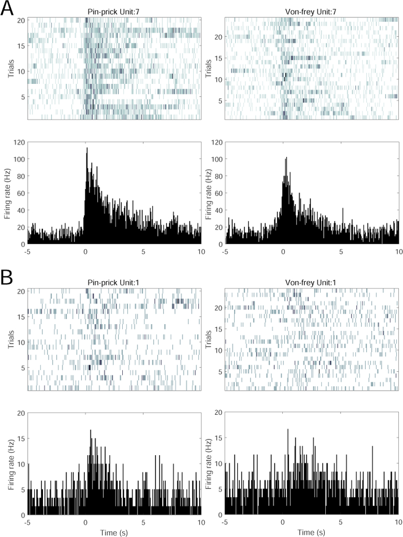
Examples of single S1 and ACC neuronal responses to noxious (pain) stimulus (pin prick) and non-noxious stimulus (von Frey, 2g). (A) One S1 unit’s spike raster (top) and peri-stimulus time histogram (PSTH, bottom) to pin prick (left) and van Frey (right). (B) One ACC unit’s spike raster and PSTH to pin prick and van Frey.
3.2. Trial Variability in Population Response to Pain Stimuli
At both single cell and population levels, neuronal re-sponses may be highly variable between trials within the same recording session (Chen et al. 2017a). As an illustrated example, we trained a total of 25 PLDS models based on 25 trials of pain stimulus (150 mW laser stimulation, 10 s per trial; Session 1 in Table 1). To test trial variability, we then apply each model to all 25 pain stimulus trials to detect the change points induced by pain stimuli, yielding a binary 25-by-25 matrix, with 1 and 0 representing true positive (TP) and false negative (FN), respectively (Fig. 2). A high percentage of 1’s in the matrix entries imply that the robustness of the model despite the data non-stationarity. In this example, 74% of entries in the TP/FN matrix show TPs and 72% of entries in the FP/TN matrix show TNs. Across each column of the TP/FN matrix in Fig. 2A, the majority of entries show agreement in TPs, justifying the use of majority rule. Notably, the entries of the banded upper diagonal (containing models trained from previ-ous 3 trials) are predominantly TPs. If a model is very poor, it will fail most good trials (e.g., the 7th row of TP/FN matrix). Similarly, we use the trained models to test non-pain stimulus trials (50 W laser stimulation) and report the FP/TN (Fig. 2B). Across each column of the FP/TN matrix, the majority of entries also show agreement in TNs.
Fig. 2.
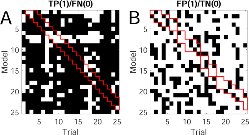
(A) Detection results of the true positive (TP) matrix. Each entry of the matrix denote the detection re-sult from one model (row) applied to one trial (column). Black/white color denotes TP/FN. (B) Detection results of the false positive (FP) matrix. Black/white color denotes FP/TN. In both panels, the red banded diagonal marks the results using models trained from previous 3 trials.
Note that in an online BMI setting, we can only use previously trained models to test the current trial. As such, this predicted detection performance will be less accurate than the off-line detection result (i.e., estimated from the current trial), and the trial-by-trial variability will inevitably affect the predicted detection performance.
3.3. Constraints on Computing Time and Data
For online BMI experiments, we often train the model on the fly based on previous trials. For a fixed model size, it costs more CPU time to train the model with more data or trials (Fig. 3A). Typically, it CPU time scales linearly with the size of training samples. Therefore, with real-time constraint on CPU and memory storage, it is more desirable to train each model with small number of trials. Our proposed strategy of ECPDs uses multiple models, each trained with one single experimental trial.
Fig. 3.
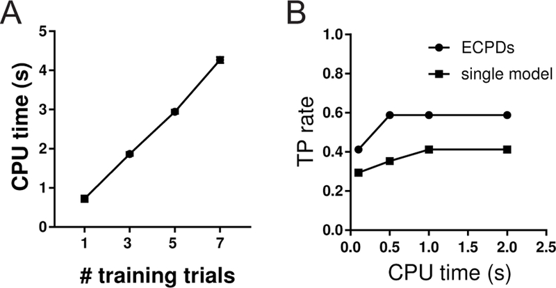
(A) CPU time scales linearly with the number of training data/trials. Here a total of 50 EM iterations are run for model estimation of 28 rat ACC units (from Session 7). (B) Comparison of TP between single-model and ensemble detection with a fixed CPU time constraint in model training.
In addition, with a fixed computing time constraint or the same amount of training time, the ECPDs may produce better detection performance (e.g., TP, FN or AUROC) than the single-model detection trained with multiple experimental trials (Fig. 3B). Therefore, the constraints on computing and memory resources in online BMI experiments favor the ensemble detection strategy.
4. Results
4.1. Computer Simulations
4.1.1. Setup 1: Impact of trial variability and SNR
First, we investigate the impact of trial-by-trial variability on model estimation and detection. We generate population spike trains of C = 24 units using a PLDS model with assumed ground truth. Each trial lasts 10 s and consists of 4 pain-modulated units (all positively modulated), with randomly generated vector c and d in Eq. (2). The values c and d are set within a predefined range to keep the Poisson spike count at each time bin less than 8. The duration of pain stimulus is 2 s. To cre-ate trial variability, we simulate different configurations where the specified number of coefficients in vector c as-sociated with the pain-modulated neurons vary across trials. Without the loss of generality, we define
Class 1: pain-modulated unit index ∈ {1, 2, 3, 4}
Class 2: non-pain-modulated unit index ∈ {5, 6}
Class 3: non-responsive unit index ∈ {7, 8, . . . , }
In the remaining computer simulations, we will use this terminology to distinguish the three classes of neurons.
For the TP experiment, we train n = 100 mod-els using all 100 randomly generated trials. Next, we apply all models to detect changes in all trials, yield-ing a n × n matrix for each dataset. We compute the average detection results based on either single detector or ECPDs using the majority vote. In this case, the testing set and training set are identical. The de-tailed results are summarized in Table 2 and Fig. 4A. As seen in the table, at nearly all configurations, the ECPDs based on the majority vote improves the detec-tion accuracy in TP. In the case of low trial variability (Datasets 1–4), the single model already achieves a good performance, so the difference between the single model and ensemble methods is small. In the medium (Datasets 5–10) and high (Datasets 11–14) variability trials, we see varying degrees of improvement in the en-semble method. Generally, the degree of improvement is greater in the presence of higher trial-by-trial vari-ability. In an extreme condition where all Class-1 units are varying across trials (i.e., the highest trial variability for Class-1 units), the performance of single model drop dramatically, and the performance of ensemble method is even worse. For Dataset 15 (the extreme high trial variability), the TP rate of ensemble detection is worse than that of the single-model detection due to lack of “consistency” across trials, implying a very low SNR. In addition, among all 400 trials of high variability (Datasets 11–14), about 75% of trials benefit from the majority vote rule (i.e., number of models detect-ing TP is greater than 50), whereas 25% of trials fail, consistent with the averaged TP rate (i.e., the mean of 51%, 69%, 84%, 84%) in Table 1. Furthermore, these 400 high-variability trials are tested from 100 trained models, change points of 288 trials can be detected by more than 50 models (Fig. 4B), suggesting the beneficial use of majority vote rule. Put together, this finding implies that ensemble detection may improve the TP rate in the context of online experiment.
Table 2.
Summary of simulation experiments (setup 1, C = 24). The smaller the number of invariant Class-1 units, the higher trial-variability within a specific data set. Datasets 1–4: low trial variability; Datasets 5–10: medium trial variability; Datasets 11–14: high trial variability. Each dataset consists of 100 Monte Carlo trials.
| Dataset | #invariant Class-1 units |
invariant Class-1 units |
TP (single) |
TP (ensemble) |
|---|---|---|---|---|
| 1 | 3 | 1, 2, 3 | 95% | 98% |
| 2 | 3 | 1, 2, 4 | 93% | 94% |
| 3 | 3 | 1, 3, 4 | 96% | 96% |
| 4 | 3 | 2, 3, 4 | 95% | 95% |
| 5 | 2 | 1, 2 | 75% | 86% |
| 6 | 2 | 1, 3 | 79% | 87% |
| 7 | 2 | 1, 4 | 85% | 88% |
| 8 | 2 | 2, 3 | 87% | 93% |
| 9 | 2 | 2, 4 | 77% | 81% |
| 10 | 2 | 3, 4 | 84% | 86% |
| 11 | 1 | 1 | 52% | 51% |
| 12 | 1 | 2 | 56% | 69% |
| 13 | 1 | 3 | 67% | 84% |
| 14 | 1 | 4 | 75% | 84% |
| 15 | 0 | 46% | 34% |
Fig. 4.
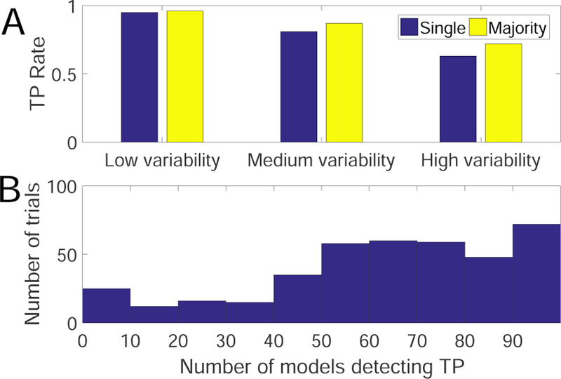
Result of simulation setup 1. (A) Comparison of average performance between the single detector and ECPDs using the majority vote under low (with 3 invariant units), medium (with 2 invariant units) and high (with 1 invariant unit) trial-by-trial variability. (B) Histogram of the number of high-variability trials (Datasets 11–14, 400 trials in total) that can be detected as TPs. Each trial is tested with 100 trained models. The trials that benefit from the majority vote are located within the right half of distribution (i.e., support > 50).
To investigate the impact of noise on change-point detection, following the simulation setup 1, we add in-dependent Poisson noise to population spike activity across time and units. We vary the noise variance or equivalently the SNR = 10 log10 son mean is equal to variance), where the SNR is as-sumed constant across trials. We repeat the experiment in simulation setup 1 and compare the TP rate be-tween the single-model detector and ECPDs. As seen in Fig. 5, ECPDs outperform the single-model detector at medium and high trial variabilities with varying SNRs; however, the superiority of ensemble learning is lost in the presence of high trial variability together with very low SNR (i.e., −5 dB and 0 dB). Therefore, ensem-ble detection has a poor performance due to the high trial-variability in both “signal” and “baseline”, since a higher variance in baseline will decrease the Z-score and make it harder to cross the significance threshold. Put together, this finding implies that ensemble detection may work robustly for a wide range of practical BMI conditions, given varying degrees of trial variability and medium-to-high SNR.
Fig. 5.
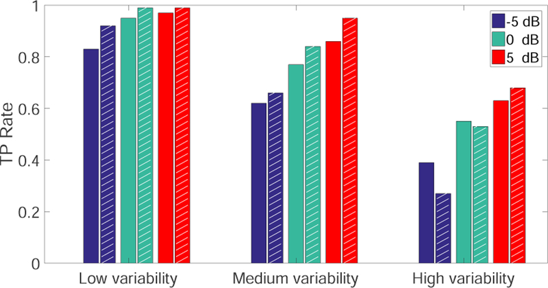
Comparison of the average TP rate between the single model detector and ECPDs (shaded bars) under different SNR levels and trial-by-trial variabilities (computer simulation setup 1).
4.1.2. Setup 2: Impact of mixed selectivity
Next, we use a similar setup but with fewer units (C = 12) to assess the FP rate in change point detection. In the training trials, it is assumed that two Class-2 units fire in response to a presumed non-painful stimulus (0.5 s duration) during the baseline with probability q, and these two Class-2 units do not overlap with the four Class-1 units mentioned above. We vary the probability q ∈ {0.1, 0.25, 0.5, 1} and simulate n = 100 training and testing trials. In the testing trials, we generate pop-ulation spike responses with only “positive” responses from these two Class-2 units, whereas the firing rates of remaining 10 units are the same as baseline. We train 100 models from all training trials and test them on all 100 testing trials, from which the FP rate is computed using either single detector or ECPDs. As seen in Table 3, ECPDs significantly reduce the FP rate based on the majority vote for a wide range of q values lower than 1. An example is shown in Fig. 6. In an extreme condition when q = 1, the model cannot distinguish between Class-1 and Class-2 neuronal responses, resulting in degraded performance in ensemble detection. This finding implies that ensemble detection may potentially reduce the FP rate in the presence of Class-2 units given a “noisy” baseline.
Table 3.
Summary of simulation experiments (setup 2, C = 12). A higher probability q implies a lower SNR in the baseline period among the training trials. Each dataset consists of 100 Monte Carlo trials.
| Dataset | prob. q | TP (single) |
FP (single) |
FP (ensemble) |
|---|---|---|---|---|
| 16 | 1.0 | 85% | 44% | 25% |
| 17 | 0.5 | 85% | 27% | 0% |
| 18 | 0.25 | 84% | 16% | 0% |
| 19 | 0.1 | 84% | 9% | 0% |
Fig. 6.
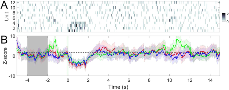
An example of simulation setup 2. (A) Simulated spike count observations of C = 12 units. The first 10-s sample points define the a training trial, whereas the last 10-s samples define a test trial that consists of a non-pain stimulus during [10, 11] s. (B) The Z-score trace derived from the PLDS model trained from 3 preceding trials (n−1, red; n − 2, green; n − 3, blue). In this example, only 1 out of 3 models detects FP. Shaded area denotes the baseline for computing the Z-score. Horizontal dashed lines denote the ±1.65 threshold.
4.2. Neuroscience Experiments for Detecting Acute Pain Signals
Furthermore, we validate our approach using experimental recordings from freely behaving rats under the experimental protocol described in Section 2.1. To assess the detection performance, we compute the TP and FP rates, as well as the AUROC (area under receiver operating characteristic) statistic. For computing the TP/FP statistics, we use the data within the period [0, 3] s, where 0 denotes the laser or stimulus onset.
4.2.1. Detection from single ACC or S1 region
In single-model detection, we use the model trained from one preceding trial to predict the current trial. For ECPDs we use three models trained from three preced-ing pain-stimulus trials to predict the current trial. Figure 7 shows a noxious stimulus example from the ACC recording, and Figure 8 shows a non-noxious stimulus example from the S1 recording. Results of all single-region recording sessions are summarized in Table 4. It is seen from the table that the ECPDs improves the AU-ROC statistic compared to the single-model detector. For the TP and FP statistics, the performance of ensemble detection either improves or remains unchanged, which may depend on the recording region, the number and characteristic of the units.
Fig. 7.
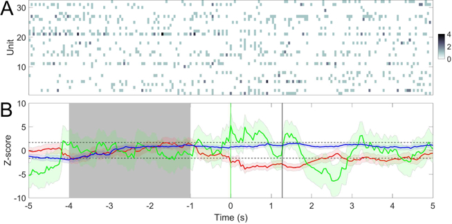
(A) Spike count observations of C = 32 ACC units (session 1). Time 0 denotes the onset of 150 mW laser stimulation. (B) Z-score statistics derived from PLDS models trained from 3 preceding trials (n − 1, red; n − 2, green; n − 3, blue). In this example, 2 out of 3 models detect the change. Shaded area denotes the baseline period ([−4, −1] s) for computing the Z-score. Vertical red and black lines denote the laser onset and paw withdrawal, respectively. Horizontal dashed lines denote the ±1.65 threshold.
Fig. 8.
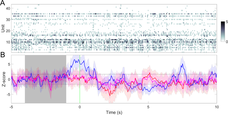
(A) A trial example of spike count observations from C = 43 S1 units (session 3). Time 0 denotes the onset of 50 mW laser stimulation. (B) Z-score statistics derived from PLDS models trained with 3 preceding trials. Model trained from the preceding trials (n − 1, red; n − 2, blue; n − 3, magenta). In this example, 1 out of 3 models detects FP. Shaded area denotes the baseline period ([−4, −1] s) for computing the Z-score. Horizontal dashed lines denote the ±1.65 threshold.
Table 4.
Comparison of AUROC, TP and FP statistics for change-point detection based on a single brain region. The TP and FP rates are computed using a significance threshold θ0 = 1.65 (i.e., P < 0.05).
| AUROC | TP | FP | |||||||||||||
|---|---|---|---|---|---|---|---|---|---|---|---|---|---|---|---|
| Session | 1 | 2 | 3 | 4 | 1 | 2 | 3 | 4 | 1 | 2 | 3 | 4 | |||
| Method | |||||||||||||||
|
single ensemble |
0.79 | 0.78 | 0.97 | 0.93 | 77% | 70% | 100% | 92% | 33% | 27% | 24% | 19% | |||
| 0.85 | 0.91 | 0.98 | 0.94 | 77% | 78% | 100% | 100% | 13% | 9% | 24% | 15% | ||||
4.2.2. Detection from joint ACC and S1 regions
Next, we focus on simultaneous recordings of ACC and S1 ensemble spike activity (Sessions 5–7 in Table 1). We compare seven detection methods: (i) Single ACC or S1 detector trained from previous 1 trial; (ii) Single ACC or S1 detector trained from previous 3 trials; (iii) Single detector with merged ACC and S1 activity trained from the previous 1 trial; (iv) Single detector with merged ACC and S1 activity trained from the previous 3 trials; (v) Ensemble of 3 detectors associated with model (i) and (iii); (vi) Two detectors (ACC+S1) based on the CCF criterion; (vii) Ensemble of 3 or 9 detectors as-sociated with model (vi). Note that by using the same amount of data, models (ii) and (iv) are compared with model (v) to determine whether the result improvement is due to the ensemble strategy or due to the use of more data.
Single vs. double brain region detection.
We first illus-trate the benefit of using the CCF between the ACC and S1 activities based on two single models derived from each area separately. Specifically, integrating in-formation from these two brain regions improves the TP rate. One example of using 150 mW laser stim-ulation is shown in Fig. 9. In this example, we track the area above the CCF threshold and determine the change point based on a predefined threshold (Fig. 9D). The optimal value of threshold θ is determined empiri-cally from the data (typically 1.5–2), depending on the trade-off between sensitivity and specificity. Moreover, integrating double-region information also reduces the FP rate. An example of such using 50 mW laser stim-ulation is shown in Fig. 10. In this example, the area above the ACC threshold is very small (Fig. 10D).
Fig. 9.
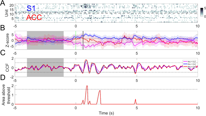
(A) A trial example of rat ACC and S1 population spike count observations with 150 mW laser stimulation. (B) Z-score curves derived from ACC (green), S1 (blue) and their merged activities (magenta). Horizontal dashed lines denote the ±1.65 threshold. Vertical red and black lines denote the laser onset and paw withdrawal, respectively. (C) Z-scored CCF derived from both regions based on different values of forgetting factor ρ; m = n = 0.5. Horizontal dashed lines indicate the mean±3SD threshold computed from the CCF during baseline (shaded area). (D) Tracking the area of CCF outside of the mean±3SD threshold in panel C (ρ = 0.6). Dashed line indicates θ = 1.6.
Fig. 10.
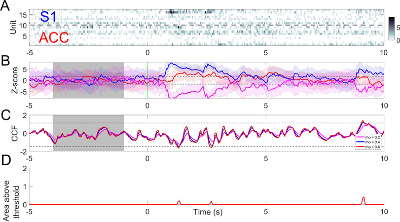
(A) A trial example of rat ACC and S1 population spike count observations with 50 mW laser stimulation at time 0. (B) Z-score curves derived from ACC (green), S1 (blue) and their merged activity (magenta). Horizontal dashed lines denote the ±1.65 threshold. (C) Z-scored CCF derived from both regions based on different values of the forgetting factor ρ; m = n = 0.5. Horizontal dashed lines indicate the mean±3SD threshold computed from the CCF during baseline (shaded area). (D) Tracking the area of CCF curve above the mean±3SD threshold in panel C (ρ = 0.6).
Single-model vs. ensemble detection on double regions.
Furthermore, we investigate if using additional models from each region may further boost the detection per-formance or enhance the robustness (as assessed by the AUROC statistic). For S1 and ACC regions, assuming each region produces N = 3 models trained by three preceding trials, we may have two possible options. The first option is to pair S1 and ACC models within indi-vidual trials, yielding three CCFs. The second option is to consider all possible pairs within and between trials, yielding a total of N 2 = 9 CCFs. We compare the AU-ROC statistics between the single-model and ensemble detection methods, using single regions only or double regions. In the ensemble method, we also compare the ECPDs using either 3 or 9 ensembles in detection. The results are summarized in Tables 5 and 6. In all results, we set the forgetting factor ρ = 0.6, m = n = 0.5. As seen in the table, the ECPDs strategy by combin-ing ensemble detection and double-region CCFs signif-icantly improves the ROC performance compared to the single-model or ensemble detection using one region alone. The benefit of ensemble detection using double-region recordings for reducing the FP rate is illustrated in Fig. 11.
Table 5.
Comparison of AUROC statistics for change-point detection based on double-region recordings (Sessions 5 and 6). The best result in each column is shown in bold font. Cases 1–4 are based on single-region detection; Cases 5–10 are based on double-region detection. Cases 6,9,10 are based on our proposed ensemble detection approach, with increasing complexity. Case 6 treats ACC+S1 as a single region, whereas Cases 9 and 10 treat ACC and S1 separately. Cases 8 and 9 are based on the same amount of training data; Cases 5 and 7 are based on the same amount of training data.
| Case | Session | 5 | 6 | 7 |
|---|---|---|---|---|
| Region | ||||
| 1 | ACC (single, 1 trial) | 0.66 | 0.63 | 0.61 |
| 2 | ACC (single, 3 trials) | 0.76 | 0.67 | 0.58 |
| 3 | S1 (single, 1 trial) | 0.74 | 0.59 | 0.58 |
| 4 | S1 (single, 3 trials) | 0.74 | 0.61 | 0.66 |
| 5 | ACC+S1 (merged, single w/ 1 trial) | 0.78 | 0.59 | 0.65 |
| 6 | ACC+S1 (merged, ensemble of 3 models) | 0.78 | 0.61 | 0.75 |
| 7 | ACC+S1 (single, each w/ 1 trial) | 0.84 | 0.67 | 0.67 |
| 8 | ACC+S1 (each w/3 trials) | 0.89 | 0.69 | 0.64 |
| 9 | ACC+S1 (each w/ensemble of 3 models) | 0.91 | 0.70 | 0.81 |
| 10 | ACC+S1 (each w/ensemble of 9 models) | 0.90 | 0.67 | 0.84 |
Table 6.
Comparison of TP and FP statistics (Sessions 5 and 6) based on varying statistical criteria or thresholds. Here, θ0 denotes the Z-score threshold, and θ denotes the threshold for the cumulated area of CCF above the mean±3SD statistic in baseline. In all single detectors, only 1 preceding trial is used to train the model; whereas in all ECPDs, the ensemble of 3 models is used. The optimal choice is shown in bold font.
| Session 5 |
P < 0.05 (θ0 = 1.65) |
P < 0.01 (θ0 = 2.33) |
P < 0.001 (θ0 = 3.08) |
|||
|---|---|---|---|---|---|---|
| TP | FP | TP | FP | TP | FP | |
| ACC (single) | 31% | 27% | 25% | 13% | 13% | 7% |
| ACC (ensemble) | 31% | 7% | 25% | 0% | 13% | 0% |
| S1 (single) | 88% | 40% | 63% | 33% | 50% | 20% |
| S1 (ensemble) | 88% | 40% | 69% | 20% | 63% | 20% |
| ACC+S1 (merged, single) | 88% | 53% | 81% | 33% | 63% | 20% |
| ACC+S1 (merged, ensemble) | 88% | 53% | 81% | 20% | 63% | 20% |
|
θ = 1 |
θ = 1.6 |
θ = 2 |
||||
| TP | FP | TP | FP | TP | FP | |
| ACC+S1 (separate, single) | 63% | 27% | 56% | 13% | 56% | 13% |
| ACC+S1 (separate, ensemble) | 75% | 13% | 75% | 7% | 63% | 7% |
| Session 6 |
P < 0.05 (θ0 = 1.65) |
P < 0.01 (θ0 = 2.33) |
P < 0.001 (θ0 = 3.08) |
|||
| TP | FP | TP | FP | TP | FP | |
| ACC (single) | 41% | 14% | 24% | 5% | 18% | 5% |
| ACC (ensemble) | 29% | 10% | 18% | 5% | 12% | 0% |
| S1 (single) | 100% | 67% | 71% | 50% | 59% | 42% |
| S1 (ensemble) | 100% | 57% | 71% | 48% | 53% | 48% |
| ACC+S1 (merged, single) | 100% | 71% | 71% | 52% | 53% | 38% |
| ACC+S1 (merged, ensemble) | 100% | 71% | 76% | 48% | 47% | 43% |
| θ = 1 | θ = 1.6 | θ = 2 | ||||
| TP | FP | TP | FP | TP | FP | |
| ACC+S1 (separate, single) | 71% | 48% | 65% | 43% | 59% | 38% |
| ACC+S1 (separate, ensemble) | 76% | 43% | 71% | 38% | 65% | 33% |
| Session 7 |
P < 0.05 (θ0 = 1.65) |
P < 0.01 (θ0 = 2.33) |
P < 0.001 (θ0 = 3.08) |
|||
| TP | FP | TP | FP | TP | FP | |
| ACC (single) | 59% | 35% | 41% | 35% | 24% | 24% |
| ACC (ensemble) | 59% | 6% | 35% | 6% | 24% | 6% |
| S1 (single) | 24% | 12% | 6% | 0% | 6% | 0% |
| S1 (ensemble) | 18% | 6% | 6% | 0% | 0% | 0% |
| ACC+S1 (merged, single) | 58% | 35% | 47% | 35% | 35% | 18% |
| ACC+S1 (merged, ensemble) | 53% | 24% | 35% | 12% | 18% | 0% |
|
θ = 1 |
θ = 1.6 |
θ = 2 |
||||
| TP | FP | TP | FP | TP | FP | |
| ACC+S1 (separate, single) | 76% | 53% | 71% | 47% | 71% | 47% |
| ACC+S1 (separate, ensemble) | 88% | 29% | 65% | 24% | 53% | 18% |
Fig. 11.
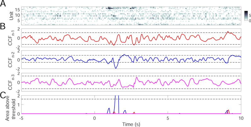
A trial example of ensemble detection based on simultaneous ACC and S1 recordings. (A) population spike count observations with 50 mW laser stimulation at time 0. (B) Z-scored cross-correlation function (CCF) based on trained models from preceding 3 (N − 1, n − 2 and n − 3) trials. In all examples, ρ = 0.6, m = n = 0.5. Horizontal dashed lines indicate the mean±3SD threshold. (C) The area of three CCF curves above their respective mean±3SD thresholds in baseline. Color matches the color from respective models in panel B. In this example, only 1 out of 3 models detects FP.
Result comparison on AUROC, TP and FP.
From Table 5, for both single or ensemble detection, it is noted that using more data generally improves the AUROC performance. In the case of single region (S1 or ACC), adding more trials in single detectors has a comparable performance with the ECPDs. However, in the case of double regions, the ECPDs is consistently better than the single detector based on the same amount of data. Overall, the best AUROC performance is produced by the ECPDs using double regions (i.e., the last two rows of Table 5). The second optimal performance is given by two single detector models (ACC+S1, separate de-coding, each with 3 trials), which is consistently better than the result of one single detector model (ACC+S1, merged decoding).
When comparing the AUROC performance using the same amount of data, the proposed ECPDs still have advantage for the sake of real-time BMI applications. From a computational point of view, our proposed ensemble detection strategy requires a model up-date based on the previous 1 trial, whereas the double-region single detector strategy would requires a model update based on the previous 3 trials. From a memory point of view, our ensemble strategy requires storing 2 models and updating 1 model with single-trial recordings, which is preferred compared with updating a single model using 3-trial recordings previously stored.
In terms of TP and FP, several points in Table 6 are noteworthy:
-
–
When the number of S1 or ACC units is small, the single-model detection performance using one brain region alone is rather poor. Generally, the S1 has higher sensitivity and FP rates; the ACC has lower TP rates. In addition, the TP or FP performance of ensemble detection shows little change or may even degrade.
-
–
The single-model detection based on double-region recordings generally improves the TP and FP rates compared with their single-region counterparts.
-
–
For double-region recordings, ensemble detection fur-ther improves the single-model detection in TP and FP rates, achieving a good trade-off between high TP and low FP rates.
-
–
In general, if the TP/FP rate of single-model detec-tors is greater than 50%, then the ensemble detec-tion will further improve the TP/FP rate. However, if the TP/FP of single-model detectors is very poor at the first place (e.g., <50%), then the ensemble de-tection will mostly likely degrade the TP/FP rate.
It is also noted that even the best results of Sessions 5 and 6 may be unsatisfactory for the targeted detection goal in BMI experiments. The reason may be due to an insufficient number of recorded units in each region, thereby limiting the detection performance based on the ACC or S1 alone. This reasoning was partially confirmed with the result of Session 7 in Table 6. Mean-while, the results from single-region recording sessions (see Table 5) also show that increasing the unit yield im-proves the overall detection performance of S1 or ACC in all categories.
4.2.3. Selection of free hyperparameters
In the double-region detection rule, several hyperpa-rameters: m, n, ρ (forgetting factor), and θ (threshold) need to be determined. The exponent parameters m and n are used to scale up or down the Z-score value, we suggest using 0.5. The forgetting factor ρ determines the smoothness of CCF curve, but the detection result is robust with respect to a wide range of ρ, we use ρ = 0.6 and find that it works well in all experimental recordings.
The choice of threshold θ determines the TP, FP and AUROC statistics. In practice, we systematically vary θ and select its optimal value based on the ROC curve (the nearest point closest to the upper left corner). Our empirical observations have shown that a threshold be-tween 1.5 and 2 yields good overall performances (see Table 6).
To test the generalization of these hyperparameters, we use the ROC curve to identify the optimal val-ues from one recording session, and then apply them to another recording session. The results are shown in Table 7. Comparing the results in Tables 6 and 7, it is found that the results are similar or nearly identical, suggesting that these parameters are quite robust across different recording sessions.
Table 7.
Testing generalization in cross-section analysis using simultaneous recordings of two brain regions (Sessions 5 and 6). In this case, the optimal hyperparameters θ0 and θ are determined from one session (based on the ROC curve) and tested on the other session.
| Session 5→Session 6 |
Session 6→Session 5 |
|||
|---|---|---|---|---|
| TP | FP | TP | FP | |
| ACC+S1 (merged, single) | 100% | 76% | 88% | 53% |
| ACC+S1 (merged, ensemble) | 100% | 71% | 88% | 53% |
| ACC+S1 (separate, single) | 65% | 43% | 56% | 13% |
| ACC+S1 (separate, ensemble) | 71% | 38% | 75% | 7% |
4.3. Detection by integration of spikes and LFP
To illustrate the benefit of integrating multi-modal information from ensemble spikes and LFP, we test our ensemble detection strategy on one recording session (Session 7). To further improve the TP and FP rates, we apply the designed ERP detector independently to the ACC and S1 regions. For a fair comparison, we use only a single model for each region. Combining the SVM detector for ACC/S1 evoked-ERP detection (Section 2.6) with the spike-based CCF detector trained from the previous one trial, we employ the ensemble detec-tion strategy using a majority vote rule (i.e., two out of three detectors). One trial example of 250 mW laser stimulation is illustrated in Fig. 12. As a result, by combining decisions from multiple (spike+LFP) inde-pendent detectors, the TP and FP rates are 88% and 29%, respectively—which are comparable with the re-sults derived from another ensemble detection strategy based on multiple ACC+S1 spike-only models (last row in Table 6). In contrast, the single model-based detec-tion strategy based on spike alone has the TP rate of 76% and FP rate of 53%; on the other hand, LFP-alone detection depends on the exact decision strat-egy, and often suffers from a high false discovery rate during baseline (see Fig. 12C). Notably, in this figural example, detection latency based on evoked-ERPs is improved from 1 s to 800 ms. Therefore, integration of multi-modal information using an ensemble detection strategy may improve not only the detection accuracy but also the detection latency.
Fig. 12.
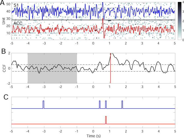
A single-trial example of ensemble detection based on simultaneous ACC and S1 recordings. (A) population spike count observations with 250 mW laser stimulation at time 0. The band-passed (2–20 Hz) LFP traces from the ACC (red) and S1 (blue) are overlaid over the ensemble spike count observations. (B) Z-scored cross-correlation function (CCF) based on single models derived from the previous one trial. ρ = 0.6, m = n = 0.5. Horizontal dashed lines indicate the mean±3SD threshold. Shaded area represents the baseline. Vertical line (∼ 1 s) indicates the time of detection upon reaching the area threshold. (C) Pain-evoked ERP detection using the SVM for the ACC (red) and S1 (blue) areas. Based on the majority vote, the detection latency of pain signals is around 800 ms
5. Discussion and Conclusion
In this paper, we have proposed an ensemble strat-egy of combining independent change-point detectors to achieve an ensemble or committee decision for change-point detection. While the individual detector can be derived from either unsupervised or supervised learning, the generic ensemble detection framework may accommodate multiple trials, multiple brain regions and multiple detection methods based on different signal modalities. The ensemble detection that integrates in-formation from both S1 and ACC regions produce the best detection performance, as validated by several experimental recordings. Depending on the quality of neu-ronal data, we can optimize the free hyperparameters to obtain an optimal trade-off between the detection accuracy and latency, and between the sensitivity and specificity.
For real-time BMI applications, the ensemble detection strategy (for either single or double regions) is appealing from both computational and memory consid-erations, as compared with the single-model detection using the same amount of data. Overall, the ECPDs can improve the robustness of detection at the mini-mum computational and memory cost.
More specifically, several points on the ensemble de-tection strategy are highlighted here:
-
–
ECPDs allow us to use more data given the same amount of training time (Fig. 3).
-
–
Given the same amount of training time, EPCDs outperform single detectors in scenarios with high trial variability (or non-stationarity), low SNR, and mixed selectivity of neuronal responses (Figs. 4–6).
-
–
ECPDs outperform or perform at least as well as single detectors based on based on the same amount training data (Table 5) or less training time (Fig. 3B). This is true for single and double-region decoding.
-
–
ECPDs can be beneficial when integrating neural recordings from spikes and LFP (Fig.12).
5.1. Integration of S1 and ACC for Pain Detection
In the present experiment, we have formulated the de-tection of pain signals as a change-point detection problem. In this context, integrating information from the S1 and ACC for detecting pain signals is critical. Previous neuroimaging and physiological data have suggested that the S1 and ACC are the two most important brain regions in responding pain stimuli. Specifically, S1 encodes the sensory-discriminative component of pain, and ACC encodes the affective-emotional component. Since there is no single brain region with pain-specific or pain-exclusive neuronal responses, it is critical to record two (or more) brain regions with complementary information, where their ensemble spikes and LFPs are both important for detecting pain signals.
5.2. Computational Consideration
For ensemble learning or committee decision, the selec-tion of decision rule is important to the ultimate de-tection accuracy, especially in TP and FP. In BMI ap-plications, we may adapt our choices depending on the SNR or practical need. To improve the online detection speed, we can use the particle filter or sequential Monte Carlo methods (Hu et al. 2018). When Monte Carlo sampling is employed and the number of ensemble de-tectors is large, it may pose a computational challenge in BMI applications. For instance, to train a PLDS model with 50 units and 15-s data points, it often takes around 30 s to run the EM algorithm for 500 itera-tions (written in custom C code, Intel i7–4700 quad-core CPU processor 3.4 GHz and 32 GB RAM). For a further computational speedup, we may consider mod-ern digital signal processing (DSP) technologies with optimized libraries.
There is also a trade-off between the detection accu-racy (FP, FN) and latency. According to our ensemble strategy (for either single or double regions), the detec-tion accuracy is improved at the expense of longer de-tection latency. On the other hand, if we aim to shorten the detection latency (using a shorter observation duration), the FP or FN rate will likely increase. Specifi-cally, we need to optimize the free hyperparameters to achieve the desired performance (section 4.2.3).
5.3. Unit Stability
In chronic neural recordings (e.g., multiple recording sessions within one day), we will encounter non-stationary issues, such as the change in unit firing rate due to neural plasticity or adaptation, electrode drifts, and unit instability. Unit instability issue is referred to the phenomenon that new spike waveforms emerge that do not match previously identified templates, or old units may disappear in a later stage. The current online spike sorting is mostly based on template matching, where the templates are pre-identified during baseline calibration prior to stimulus presentation.
For any disappeared unit that has been assigned with a weighting coefficient in vector c, we can reset the weighting coefficient to 0. For any emerged new units, we either ignore their spikes or merge them with neigh-boring units with the closest waveform (treated as the multiunit activity) and retrain the model parameters.
Currently, we are improving the custom micro drive design (2 × 32 channels, Session 7) and the unit yield (>50 units). The increase in unit yield may also pose more practical considerations in computational speed and unit selection (e.g., removal of non-informative units). With more units simultaneously recorded from the ACC and S1, we expect to further improve the TP and FP rates based on an ensemble detection strategy. In addition, we are developing a software interface to monitor the online-sorted unit activity in BMI experiments.
Acknowledgements
The authors thank Eric J. Robinson for English proofreading. The work was supported by the NSF-CRCNS grant IIS-130764 (Z.C.), NSF-NCS grant #1835000 (Z.C., J.W.), NIH grants R01-NS100016 (Z.C., J.W.), R01-MH118928 (Z.C.) and R01-GM115384 (J.W.), as well as the China’s Natural Science Foundation #31627802 and Funda-mental Research Funds for the Central Universities (Y.C.).
Contributor Information
Zhengdong Xiao, Department of Instrument Science and Technology, Zhejiang University, Hangzhou, Zhejiang 310027, China; Department of Psychiatry, New York University School of Medicine, New York, NY 10016, USA.
Sile Hu, Department of Instrument Science and Technology, Zhejiang University, Hangzhou, Zhejiang 310027, China; Department of Psychiatry, New York University School of Medicine, New York, NY 10016, USA.
Qiaosheng Zhang, Department of Anesthesiology, Perioperative Care, and Pain Medicine, New York University School of Medicine, New York, NY 10016, USA.
Xiang Tian, Department of Instrument Science and Technology, Zhejiang Provincial Key Laboratory for Network Multimedia Technologies, Key Laboratory for Biomedical Engineering of Ministry of Education of China, Zhejiang University, Hangzhou, Zhejiang 310027, China.
Yaowu Chen, Department of Instrument Science and Technology, Zhejiang Provincial Key Laboratory for Network Multimedia Technologies, Key Laboratory for Biomedical Engineering of Ministry of Education of China, Zhejiang University, Hangzhou, Zhejiang 310027, China.
Jing Wang, Department of Anesthesiology, Perioperative Care, and Pain Medicine, New York University School of Medicine, New York, NY 10016, USA.
Zhe Chen, Department of Psychiatry, Department of Neuroscience and Physiology, New York University School of Medicine, New York, NY 10016, USA.
References
- Aminikhanghahi S & Cook DJ (2017). A survey of meth-ods for time series change point detection. Knowledge Information Systems 51(2), 339–367. [DOI] [PMC free article] [PubMed] [Google Scholar]
- Bushnell MC, Ceko M & Low LA (2013). Cognitive and emotional control of pain and its disruption in chronic pain. Nature Review Neuroscience 14, 502–511. [DOI] [PMC free article] [PubMed] [Google Scholar]
- Buzsaki G, Anastassiou CA & Koch C (2012). The origin of extracellular fields and currents—EEG, ECoG, LFP and spikes. Nature Reviews Neuroscience 13, 407–420. [DOI] [PMC free article] [PubMed] [Google Scholar]
- Chen Z, ed. (2015). Advanced State Space Methods in Neural and Clinical Data, Cambridge University Press. [Google Scholar]
- Chen Z & Wang J (2016). Statistical analysis of neuronal population codes for encoding acute pain. In Proceedings of IEEE ICASSP, pp. 829–833.
- Chen Z, Hu S, Zhang Q & Wang J (2017b). Quickest detection for abrupt changes in neuronal ensemble spiking activity using model-based and model-free approaches. In Proceedings of 8th International IEEE/EMBS Conference on Neural Engineering (NER’17), pp. 481–484.
- Chen Z, Zhang Q, Tong APS, Manders TR & Wang J (2017a). Deciphering neuronal population codes for acute thermal pain. Journal of Neural Engineering 14(3), 036023. [DOI] [PMC free article] [PubMed] [Google Scholar]
- Cheppudira BP (2006). Characterization of hind paw licking and lifting to noxious radiant heat in the rat with and without chronic inflammation. Journal of Neuroscience Methods 155, 122–125. [DOI] [PubMed] [Google Scholar]
- Copits BA, Pullen MY & Gereau RW IV (2016). Spotlight on pain: optogenetic approaches for interrogating somatosensory circuits. Pain 157, 2424–2433. [DOI] [PMC free article] [PubMed] [Google Scholar]
- Daou I, Tuttle AH, Longo G, Wieskopf JS, Bonin RP, Ase AR, Wood JN, De Koninck Y, Ribeiroda Silva A, Mogil JS & Sgula P (2013). Remote optogenetic activation and sensitization of pain pathways in freely moving mice. J. Neurosci 33, 18631–18640. [DOI] [PMC free article] [PubMed] [Google Scholar]
- Deuis JR, Dvorakova LS & Vetter I (2017). Methods used to evaluate pain behaviors in rodents. Frontiers in Molecular Neuroscience 10, 284. [DOI] [PMC free article] [PubMed] [Google Scholar]
- Dietterich TG (2000). Ensemble methods in machine learning. In Gayar NE, Kittler J & Roli F, eds, Multiple Classifier Systems, Springer. [Google Scholar]
- Fraser GW, Chase SM, Whitford A & Schwartz AB (2009). Control of a brain-computer interface without spike sorting. Journal of Neural Engineering 6, 055004. [DOI] [PubMed] [Google Scholar]
- Goodman IN & Johnson DH (2008). Information theo-retic bounds on neural prosthesis effectiveness: The importance of spike sorting. In Proc. ICASSP’08, pp. 5204–5207.
- Gross J, Schnitzler A, Timmermann L & Ploner M (2007). Gamma oscillations in human primary somatosensory cortex reflect pain perception. PLoS Biology 5, e133. [DOI] [PMC free article] [PubMed] [Google Scholar]
- Gu L, Uhelski ML, Anand S, Romero-Ortega M, Kim YT, Fuchs PN & Mohanty SK (2015). Pain inhibi-tion by optogenetic activation of specific anterior cingulate cortical neurons. PLoS ONE 10, e0117746. [DOI] [PMC free article] [PubMed] [Google Scholar]
- Harris-Bozer AL & Peng YB (2016). Inflammatory pain by carrageenan recruits low-frequency local field potential changes in the anterior cingulate cortex. Neuroscience Let-ters 632, 8–14. [DOI] [PubMed] [Google Scholar]
- Hu S, Zhang Q, Wang J & Chen Z (2017). A real-time rodent neural interface for deciphering acute pain signals from neuronal ensemble spike activity. In Proc. 51st Asilomar Conf. Signals, Systems, and Computers, pp. 93–97.
- Hu S, Zhang Q, Wang J & Chen Z (2018). Real-time particle filtering and smoothing algorithms for detecting abrupt changes in neural ensemble spike activity. Journal of Neurophysiology 149(4), 1394–1410. [DOI] [PMC free article] [PubMed] [Google Scholar]
- Iyer SM, Vesuna S, Ramakrishnan C, Huynh K, Young S, Berndt A, Lee SY, Gorini CJ, Deisseroth K & Delp SL (2016). Optogenetic and chemogenetic strategies for sustained inhibition of pain. Scientific Reports 6, 30570. [DOI] [PMC free article] [PubMed] [Google Scholar]
- Jaffe A, Nadler B & Kluger Y (2015). Estimating the accuracies of multiple classifiers without labeled data. In AISTAT’15.
- Kittler J, Hatef M, Duin RPW & Matas J (1998). On combining classifiers. IEEE Trans. Patt. Anal. Mach. Intell 20(3), 226–239. [Google Scholar]
- Kopepcke L, Ashida G & Kretzberg J (2016). Single and multiple change point detection in spike trains: comparison of different CUSUM methods. Frontiers in Systems Neuroscience 10, 51. [DOI] [PMC free article] [PubMed] [Google Scholar]
- Kuncheva LI (2004). Combining Pattern Classifiers: Methods and Algorithms, Wiley. [Google Scholar]
- Kuo CC & Yen CT (2005). Comparison of anterior cingulate and primary somatosensory neuronal responses to noxious laser-heat stimuli in conscious, behaving rats. Journal of Neurophysiology 94, 1825–1836. [DOI] [PubMed] [Google Scholar]
- Lee M, Manders TR, Eberle SE, Su C, D’amour J, Yang R, Lin HY, Deisseroth K, Froemke RC & Wang J (2015). Activation of corticostriatal circuitry relieves chronic neuropathic pain. Journal of Neuroscience 35(13), 5247–5259. [DOI] [PMC free article] [PubMed] [Google Scholar]
- Liu Y & Yao X (1999). Ensemble learning via negative correlation. Neural Networks 12(10), 1399–1404. [DOI] [PubMed] [Google Scholar]
- Macke JH, Buesing L & Sahani M (2015). Estimating state and parameters in state space models of spike trains. In Chen Z, ed., Advanced State Space Methods in Neural and Clinical Data, Cambridge University Press. [Google Scholar]
- Mallat S (2008). A Wavelet Tour of Signal Processing: the Sparse Way, 3rd edn, Academic Press. [Google Scholar]
- Parisi F, Strino F, Nadler B & Kluger Y (2014). Ranking and combining multiple predictors without labeled data. Proc. Natl. Acad. Sci. USA 111(4), 1253–1258. [DOI] [PMC free article] [PubMed] [Google Scholar]
- Peng WW, Xia XL, Yi M, Huang G, Zhang Z, Iannetti G & Hu L (2017). Brain oscillations reflecting pain-related behavior in freely-moving rats. Pain 159(1), 106– 118. [DOI] [PMC free article] [PubMed] [Google Scholar]
- Perl ER (2007). Ideas about pain, a historical view. Nat. Rev. Neurosci 8, 71–80. [DOI] [PubMed] [Google Scholar]
- Pillow JW, Ahmadian Y & Paninski L (2011). Model-based decoding, information estimation, and change-point detection techniques for multineuron spike trains. Neural Computation 23(1), 1–45. [DOI] [PubMed] [Google Scholar]
- Raykar VC, Shipeng Y, Zhao LH, Valdez GH, Florin C, Bogoni L & Moy L (2010). Learning with crowds. Journal of Machine Learning Research 11, 1297–1322. [Google Scholar]
- Scholkopf B. & Smola AJ (2001). Learning with Kernels: Support Vector Machines, Regularization, Optimization, and Beyond, MIT Press. [Google Scholar]
- Taesler P & Rose M (2016). Prestimulus theta oscillations and connectivity modulate pain perception. Journal of Neuroscience 36, 5026–5033. [DOI] [PMC free article] [PubMed] [Google Scholar]
- Urien L, Xiao Z, Dale J, Bauer EP, Chen Z & Wang J (2018). Rate and temporal coding mechanisms in the anterior cingulate cortex for pain anticipation. Scientific Reports 8, 8298. [DOI] [PMC free article] [PubMed] [Google Scholar]
- Vierck CJ, Whitsel BL, Favorov OV, Brown AW & Tommerdahl M (2013). Role of primary somatosensory cortex in the coding of pains. Pain 154, 334–344. [DOI] [PMC free article] [PubMed] [Google Scholar]
- Vogt BA (2005). Pain and emotion interactions in subre-gions of the cingulate gyrus. Nat. Rev. Neurosci 6(7), 533– 544. [DOI] [PMC free article] [PubMed] [Google Scholar]
- Xie Y, Huang J & Willett R (2013). Change-point detection for high-dimensional time series with missing data. IEEE Journal of Selected Topics in Signal Processing 7(1), 12–27. [Google Scholar]
- Xu J & Brennan TJ (2011). The pathophysiology of acute pain: animal models. Curr. Opin. Anaesthesiol 24(5), 508– 514. [DOI] [PMC free article] [PubMed] [Google Scholar]
- Zhang Q, Manders T, Tong APS, Yang R, Garg A, Martinez E, Zhou H, Dale J, Goyal A, Urien L, Yang G, Chen Z & Wang J (2017). Chronic pain induces generalized enhancement of aversion. eLife 6, e25302. [DOI] [PMC free article] [PubMed] [Google Scholar]
- Zhang Q, Xiao Z, Hu S, Kulkarni P, Martinez E, Tong A, Garg A, Zhou H, Chen Z & Wang J (2018). Local field potential decoding of the onset and intensity of acute thermal pain in rats. Scientific Reports 8, 8299. [DOI] [PMC free article] [PubMed] [Google Scholar]
- Zhang Y, Wang N, Wang J-Y, Chang J-Y, Woodward DJ & Luo F (2011). Ensemble encoding of nociceptive stimulus intensity in the rat medial and lateral pain systems. Molecular Pain 7, 64. [DOI] [PMC free article] [PubMed] [Google Scholar]


