

Abstract
Magnetic resonance fingerprinting (MRF) is a technique for quantitative estimation of spin- relaxation parameters from magnetic-resonance data. Most current MRF approaches assume that only one tissue is present in each voxel, which neglects intravoxel structure, and may lead to artifacts in the recovered parameter maps at boundaries between tissues. In this work, we propose a multicompartment MRF model that accounts for the presence of multiple tissues per voxel. The model is fit to the data by iteratively solving a sparse linear inverse problem at each voxel, in order to express the measured magnetization signal as a linear combination of a few elements in a precomputed fingerprint dictionary. Thresholding-based methods commonly used for sparse recovery and compressed sensing do not perform well in this setting due to the high local coherence of the dictionary. Instead, we solve this challenging sparse-recovery problem by applying reweighted-𝓁1-norm regularization, implemented using an efficient interior-point method. The proposed approach is validated with simulated data at different noise levels and undersampling factors, as well as with a controlled phantom-imaging experiment on a clinical magnetic-resonance system.
Keywords: Quantitative MRI, magnetic resonance fingerprinting, multicompartment models, parameter estimation, sparse recovery, coherent dictionaries, reweighted 𝓁1 -norm
1. Introduction
1.1. Quantitative magnetic resonance imaging
Magnetic resonance imaging (MRI) is a medical-imaging technique, which has become a key technology for non-invasive diagnostics due to its excellent soft-tissue contrast. MRI is based on the nuclear magnetic resonance phenomenon, in which the nuclear spin of certain atoms absorb and emit electromagnetic radiation. To perform MRI, subjects are placed in a strong magnetic field, which generates a macroscopic net magnetization of the spin ensemble. Radio-frequency (RF) pulses are used to manipulate this magnetization, causing it to precess. As a result, an electro-magnetic signal is emitted, which can be measured and processed. The dynamics of the magnetization are commonly described by the Bloch equation [9]:
| (1.1) |
where ∂/∂t is a partial derivative with respect to time. Mx, My and Mz are functions of time which denote the magnetization along the three spatial dimensions. The Larmor frequency ωz is the frequency at which the spins precess. Magnetic fields, called gradient fields because they vary linearly along different spatial dimensions, are used to modify ωz and select the specific region to be imaged, as well as to encode the magnetization in the Fourier domain (see [57] for more details). The frequencies ωx and ωy are varied over time using RF pulses in order to create a specific spin evolution that makes spin-relaxation effects accessible. This evolution is governed by the time constants T1 and T2, which are tissue specific and serve as valuable biomarkers for various pathologies.
In traditional MRI techniques, a sequence of RF pulses, and hence of frequencies ωx and ωy , is designed so that the resulting signal at each voxel of an image is predominantly weighted by the values of T1 or T2. MR images obtained in this way are qualitative in nature, in contrast to other medical-imaging modalities such as computed tomography or positron emission tomography. The images consist of gray values that capture relative signal intensity changes between tissues, caused by their different T1 and T2 values, which are then interpreted by radiologists to detect pathologies. The specific numerical value at each voxel is typically subject to variations between different MRI systems and data-acquisition settings. As a result, it is very challenging to use data from current clinical MRI systems for longitudinal studies, early detection and progress-tracking of disease, and computer-aided diagnosis.
The goal of quantitative MRI is to measure physical parameters such as T1 and T2 quantitatively, in a way that is reproducible across different MRI systems [23,35,67,71]. Quantitative MRI techniques can be used to extract quantitative biomarkers [53, 56, 63] and synthesize images with standardized contrasts [26, 59]. Unfortunately, existing data-acquisition protocols for quantitative MRI often lead to long measurement times that are challenging to integrate in the clinical work-flow and as a consequence are not widely deployed.
1.2. Magnetic resonance fingerprinting
Magnetic resonance fingerprinting (MRF) [48] is a recently-proposed quantitative MRI technique to measure tissue-specific parameters within scan times that are clinically feasible. In many traditional MRI techniques, the same RF pulse is applied repeatedly, driving the magnetization into a steady state in which the signal has a fixed weighting of T1 and T2 effects. In MRF, the amplitudes of the RF pulses are varied over time to deliberately avoid a steady state of the magnetization, creating a time-dependent signal weighting. This makes it possible to estimate the relaxation times T1 and T2 quantitatively by fitting the corresponding signal model, governed by the Bloch equation (1.1). Unfortunately, it is very challenging to fit this model by directly minimizing the fitting error, as this results in a highly non-convex cost function. Instead, MRF methodology fits the model by comparing the observed time evolution of the magnetization signal to a dictionary of fingerprints, which are precomputed by solving the Bloch equation (1.1) numerically for a range of T1 and T2 relaxation times.
Current MRF methods usually operate under the assumption that only one type of tissue is present in each volume element, called voxel. However, this assumption is violated at boundaries between tissues. As mentioned previously, spatial information in MR signals is typically encoded in the Fourier domain. This domain can only be measured up to a certain cut-off frequency, which results in a limited spatial resolution, typically of the order of a millimeter. Thus, sharp boundaries between different tissues may be blurred, so that voxels close to the boundary contain several tissue compartments (see Figure 1 for a concrete example). Fitting a single-compartment model to data obtained from a voxel with multiple tissues yields erroneous parameter estimates that may not correspond to any of the contributing compartments, a phenomenon known as the partial-volume effect [72]. Consequently, single-compartment MRF methods often do not accurately characterize boundaries between tissues, as discussed by the original developers of MRF [26]. This limitation is particularly problematic in applications that require geometric measurements, such as the diagnostic of Alzheimers disease, where cortical thickness provides a promising biomarker for early detection [40].
Figure 1:
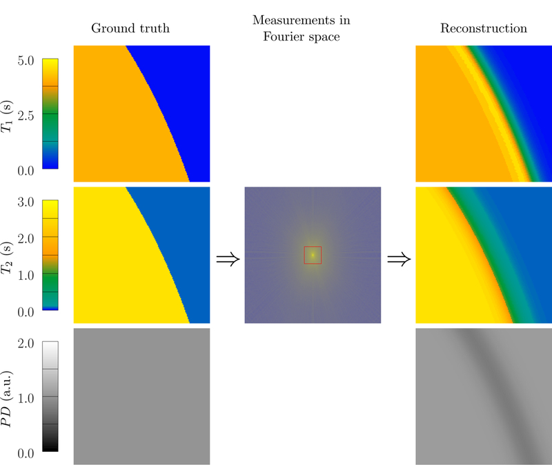
MRF reconstruction of a sharp boundary between two tissue regions with constant proton density (PD) and relaxation times corresponding to gray matter (T1 = 1123 ms, T2 = 88 ms) and cerebrospinal fluid (T1 = 4200 ms, T2 = 2100 ms) [29]. Due to the limited resolution caused by the low-pass measurements depicted by a red rectangle in the image at the center, voxels close to the boundary contain signals from the two tissues. This leads to erroneous parameter estimations near the boundary when using the standard MRF single-compartment reconstruction. A multicompartment model would be required to identify the correct relaxation times of the two contributing compartments.
The cellular microstructure of biological tissues results in multiple tissue compartments being present even in voxels that are not located at tissue boundaries. An important example is white matter in the brain, which contains extra- and intra-axonal water with similar relaxation times, as well as water trapped between the myelin sheets, which has substantially shorter relaxation times [44]. If a disease causes demyelination, the myelin-water fraction, which is the fraction of the proton density in the voxel corresponding to myelin-water, is reduced [45]. Multicompartment models capable of evaluating the myelin-water fraction are therefore useful for the diagnosis of neurodegenerative diseases such as multiple sclerosis [44, 45]. Single-compartment models cannot be applied in such settings because they fail to account for this microstructure, as illustrated in Figure 2.
Figure 2:
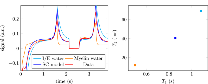
The left image shows the simulated signals corresponding to two different tissues: intra/extra (I/E) axonal water (light blue) and myelin water (orange). The signal in a voxel containing both tissues corresponds to the sum of both signals (red). A single-compartment (SC) model (blue) is not able to approximate the data (left) and results in an inaccurate estimate of the relaxation parameters T1 and T2 even in the absence of noise (right). The MRF dictionary is generated using the approach described in [3], which produces real-valued fingerprints.
It is important to note that the presence of different tissues does not necessarily result in entirely separated compartments within a voxel. In fact, one can observe chemical exchange of water molecules between compartments [1]. However, in the case of tissue boundaries, these effects play a subordinate role due to the macroscopic nature of the interfaces. Similarly, in the case of myelin-water imaging, neglecting chemical exchange is a reasonable and commonly-used assumption in literature [45]. In this work, we consider a multicompartment model that incorporates this assumption. The measured signal at a given voxel is modeled as the sum of the signals corresponding to the individual tissues present in the voxel, as in Ref. [54].
1.3. Related work
Previous works applying multicompartment estimation in the context of myelin-water imaging, applied bi exponential fitting to data obtained from a multi-echo experiment [44,45]. Other works used non-convex optimization to fit a multicompartment model to measurements from a multi-steady-state experiment [24, 25]. In the context of MR fingerprinting, the multicompartment problem has been tackled by exhaustive search in [39]. The work that lies closer to our proposed approach is [54], which also proposes to fit a multicompartment MRF model by solving sparse-recovery problems at each voxel. Ref. [54] reports that solving these sparse-recovery problems using a first order method for 𝓁1-norm minimization does not yield sparse estimates (which is consistent with our experiments, see Figure 6). They instead propose to use a reweighted-least-squares method based on a Bayesian framework to fit the multicompartment parameters to MRF data, which produces superior results, but still does not yield a sparse estimate (see Figure 9 for an example). As a result, the method tends to produce an estimate of a set of possible values for the relaxation times at each compartment, which must be post-processed to produce the parameter estimates. In contrast, we show reweighted-𝓁1-methods tend to yield sparse solutions, which can be used to estimate the relaxation parameters directly (see Section 2.4 for more details).
Figure 6:
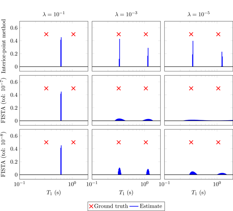
Estimates for the components of an MRF signal obtained by solving problem (2.28) for different values of the parameter λ using an interior point solver solver [36] and an implementation of FISTA [5] from the TFOCS solver [6]. The data are generated by adding i.i.d. Gaussian noise to the two-compartment MRF signal shown in Figure 5 (top left). The signal-to-noise ratio is equal to 100 (defined as the ratio between the 𝓁2 norm of the signal and the noise) or equivalently 40 dB. FISTA is terminated at an iteration k where the relative change in the coefficients falls below the chosen tolerance. It takes between 5 and 10 minutes for a single instance with a tolerance of 10−8 and 20–40 seconds with a tolerance of 10−7. CVX is run with the default precision and requires 2 seconds per instance.
Figure 9:
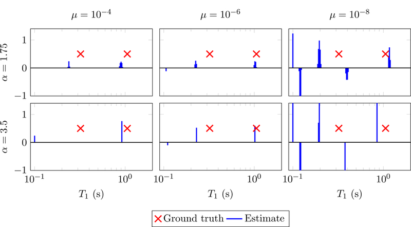
Results of applying the method in [54] to the data used in Figure 6. The underlying gamma distribution is parameterized with α ∈ {1.75,3.5} and β = 0.01 as recommended by the authors. Reconstruction is shown for a range of values of an additional parameter (µ).
Sparse linear models are a fundamental tool in statistics [33,41], signal processing [51] and machine learning [49], as well as across many applied domains [47, 78]. Most works that apply these models to recover sparse signals focus on incoherent measurements [8, 14, 17, 20, 27, 28, 37, 55, 73]. As explained in more detail in Section 2.4, this setting is not relevant to MRF where neighboring dictionary columns are highly correlated. Instead, the present work is more related to recent advances in optimization-based methods for sparse recovery from coherent dictionaries [7, 15,30,31,50, 68, 69]. Related applied work includes the application of these techniques to source localization in electroencephalography [65,80], analysis of positron-emission tomography data [38,42] and radar imaging [61]. In addition, our work combines insights from recovery methods based on reweighting convex sparsity-inducing norms [19, 76] and techniques for distributed optimization [11].
1.4. Contributions
The main contribution of this work is a method for fitting multicompartment MRF models. These models represent the requires solving a sparse linear inverse problem. We combine the following insights to solve this challenging inverse problem both accurately and efficiently:
Fitting the multicompartment model can be decoupled into multiple sparse-recovery problems–one for each voxel– using the alternating-direction of multipliers framework (see Section 2.2).
The correlations between atoms in the dictionary make it possible to compress the dictionary to decrease the computational cost (see Section 2.3).
Thresholding-based algorithms, typically used for sparse recovery and compressed sensing, do not perform well on the multicompartment MRF problem, due to the high correlation between dictionary atoms. However, 𝓁1-norm minimization does succeed in achieving exact recovery in the absence of noise as long as the problem is solved using higher-precision second-order methods (see Section 2.4).
The sparse-recovery approach can be made robust to noise and model imprecisions by using reweighted-𝓁1-norm methods (see Section 2.5).
These reweighted methods can be efficiently implemented using a second-order interior-point solver described in Section 2.6.
We validate our proposed method via numerical experiments on simulated data (see Section 3.1), as well as on experimental data from a custom-built phantom using a clinical MR system (see Section 3.2).
2. Methods
2.1. Multicompartment model
In this work, we consider the problem of estimating the relaxation times T1 and T2 via magnetic-resonance fingerprinting (MRF) [48] in situations where a voxel may contain several tissue compartments. As described briefly in Section 1.1, T1and T2 determine the time evolution of the measured nuclear-spin magnetization signal. MR systems measure the magnetization component that is per-pendicular to the external field, which is usually assumed to be aligned with the z axis [57]. For a voxel which contains only one tissue, the time evolution of this component can be approximated as a function of the values of T1 and T2
| (2.1) |
where the two-dimensional vector is represented as a complex number following the usual convention in the MRI literature. The main insight underlying MRF is that even though the mapping φ cannot be computed explicitly, it can be evaluated numerically by solving the Bloch equations (1.1). This makes it possible to build a dictionary of possible time evolutions or fingerprints for a discretized set of values of T1 and T2. We denote such a dictionary by
| (2.2) |
where t1, t2,...,tn are the times at which the magnetization signal is sampled and are the discretized T1 and T2 values respectively (there are m fingerprints in total). Small variations of T1 and T2 in Eq. (2.1) result in small changes in the magnetization signal. As a result, neighboring columns of D (i.e. fingerprints corresponding to similar T1 and T2 values) are highly correlated.
When several tissues are present in a single voxel, we assume that the different magnetization components combine additively (see the discussion at the end of Section 1.2). In that case, the magnetization vector measured at voxel j is given by
| (2.3) |
where ρ (tissue s) denotes the proton density of tissue s and S the number of tissues in the voxel. If the values of the relaxation times in each voxel are present in the dictionary, the magnetization vector can be expressed as
| (2.4) |
where N is the number of voxels in the volume of interest. The vectors of coefficients are assumed to be sparse and nonnegative: each nonzero entry in corresponds to the proton density of a tissue that is present in voxel j. The nonnegativity assumption implies that the magnetization signal from all compartments has the same complex phase, which is unwound prior to the fitting process. This neglects the effect of Gibbs ringing, due to the truncation of MR measurements in the frequency space (the lobes of the convolution kernel corresponding to the truncation may be negative). However, this issue can be mitigated by applying appropriate filtering, which makes the nonnegativity assumption reasonable in most cases.
Raw MRI data sampled at a given time do not directly correspond to the magnetization signal of the different voxels, but rather to samples from the spatial Fourier transform of the magnetization over all voxels in the volume of interest [46], a representation known as k-space in the MRI literature [74]. Staying within clinically-feasible scan times in MRF requires subsampling the image k-space and therefore violating the Nyquist-Shannon sampling theorem [48]. The k-space is typically subsampled along different trajectories, governed by changes in the magnetic-field gradients used in the measurement process. We define a linear operator that represents the linear operator mapping the magnetization at time ti to the measured data , where d is the number of k-space samples at ti. This operator encodes the chosen subsampling pattern in the frequency domain. The model for the data is consequently of the form
| (2.5) |
where we have ignored noise and model inaccuracies. If the data are acquired using multiple receive coils, the measurements can be modeled as samples from the spectrum of the pointwise product between the magnetization and the sensitivity function of the different coils [62, 66]. In that case the operator Fti also includes the sensitivity functions and d is the number of k-space samples multiplied by the number of coils.
2.2. Parameter Map Reconstruction via Alternating Minimization
For ease of notation, we define the magnetization and coefficient matrices
| (2.6) |
| (2.7) |
so that we can write (2.4) as
| (2.8) |
In addition we define the data matrix
| (2.9) |
and a linear operator ℱ such that
| (2.10) |
Note that by (2.5) the ith column of Y is the result of applying Fti to the ith row of X.
In principle, we could fit the coefficient matrix by computing a sparse estimate such that Unfortunately, this would require solving a sparse-regression problem of intractable dimensions. Instead we incorporate a variable to represent the magnetization and formulate the model-fitting problem as
| (2.11) |
| (2.12) |
| (2.13) |
where R is a regularization term to promote sparse solutions. In order to alternate between updating the magnetization and coefficient variables, we follow the framework of the alternative-direction method of multipliers (ADMM) [11]. Consider the augmented Lagrangian with respect to the constraint (2.12),ℒ
| (2.14) |
where the constant µ > 0 is a parameter and the dual variable Λ is an matrix. ADMM alternates between minimizing the augmented Lagrangian with respect to each primal variable sequentially and updating the dual variable. We now describe each of the updates in more detail. We denote the values of the different variables at iteration l by C(l), X(l) and Λ(l). More details on the implementation can be found in Ref. [2].
Updating
If we fix and Λ, minimizing over is equivalent to solving the least-squares problem
| (2.15) |
This step amounts to estimating a magnetization matrix that fits the data while being close to the magnetization corresponding to the current estimate of dictionary coefficients. The optimization problem has a closed-form solution, but due to the size of the matrices it is more efficient to solve it using an iterative algorithm such as the conjugate-gradients method [64].
Updating
If we fix and Λ, minimizing over decouples into N subproblems. In more detail, the goal is to compute a sparse nonnegative vector of coefficients for each voxel j , such that
| (2.16) |
where the left hand side corresponds to the jth column of . This collection of sparse-recovery problems is very challenging to solve due to the correlations between the columns of D. In Sections 2.4, 2.5 and 2.6 we present an algorithm to tackle them efficiently.
Updating Λ
The dual variable is updated by setting
| (2.17) |
We refer to [11] for a justification based on dual-ascent methods.
2.3. Dictionary compression
As explained in Section 2.1 nearby columns in the dictionary of fingerprints D are highly correlated. In fact, fingerprint dictionaries tend to be approximately low rank [2, 54], which means that their singular values present a rapid decay (see Figure 3 for an example). Consider the singular value decomposition
| (2.18) |
Figure 3:
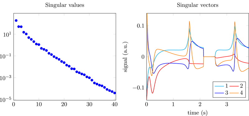
Singular values (left) and corresponding left singular vectors (right) of an MRF dictionary generated using the approach in [3,4].
where the superscript ∗ denotes conjugate transpose. If D is approximately low rank, then its column space is well approximated as the span of the first few left singular vectors (Figure 3 shows some of these singular vectors for a concrete example). Following [2, 54], we exploit this low-rank structure to compress the dictionary. Let denote the rank-k truncated SVD of D, where Uk contains the first k left singular vectors and Σk and Vk the corresponding singular values and right singular vectors. If the measured data follow the linear model , then
| (2.19) |
| (2.20) |
where is a modified linear operator and
can be interpreted as a compressed dictionary with dimensions k × m obtained by projecting each fingerprint onto the k-dimensional subspace spanned by the columns of Uk , which are depicted on the right image of Figure 3. In our experiments, D is well approximated by for values of k between 10 and 15. As a result, replacing by and D by within the ADMM framework in Section 2.2 dramatically decreases the computational cost.
2.4. Sparse estimation via 𝓁1 -norm minimization
In this section, we consider the problem of estimating the tissue parameters at a fixed voxel from the time evolution of its magnetization signal. As described in Section 2.2, this is a crucial step in fitting the MRF multicompartment model. To simplify the notation, we denote the discretized magnetization signal at an arbitrary voxel by (where n is the number of time samples) and the sparse nonnegative vector of coefficients by . In Eq. (2.16), x represents the column of corresponding to the voxel at a particular iteration l of the alternating scheme.
Let us first consider the sparse recovery problem assuming that the magnetization estimate is exact.
In that case there exists a sparse nonnegative vector c such that
| (2.23) |
Even in this simplified scenario, computing c from x is very challenging. The dictionary is overcomplete: there are more columns than time samples because the number of fingerprints m is larger than the number of time samples n. As a result the linear system is underdetermined: there are infinite possible solutions. However, we are not interested in arbitrary solutions, but rather in sparse nonnegative solutions, where c contains a small number of nonzero entries corresponding to the tissues present in the voxel.
There is a vast literature on the recovery of sparse signals from underdetermined linear measurements. Two popular techniques are greedy methods that select columns from the dictionary sequentially [52, 60] and optimization-based approaches that minimize a sparsity-promoting cost function such as the 𝓁1 norm [16, 21, 27]. Theoretical analysis of these methods has established that they achieve exact recovery and are robust to additive noise if the overcomplete dictionary is incoherent, meaning that the correlation between the columns in the dictionary is low [8,14,17,27,28,37,55,73]. Some of these works assume stronger notions of incoherence such as the restricted-isometry condition [17] or the restricted-eigenvalue condition [8].
Recall that the mapping (2.1) between the magnetization signal and the parameters of interest is smooth. As a result, when the parameter space is discretized finely to construct the dictionary, the correlation between fingerprints corresponding to similar parameters is very high. This is illustrated by Figure 4, which shows the correlations between columns for a simple MRF dictionary simulated following [3, 4]. For ease of visualization, the only parameter that varies in the dictionary is T1 (the value of T2 is fixed to 62 ms), so that the correlation in the depicted dictionary has a very simple structure: neighboring columns correspond to similar values of T1 and are, therefore, more correlated, whereas well-separated columns are less correlated. For comparison, the figure also shows the correlations between columns for a typical incoherent compressed-sensing dictionary generated by sampling each entry independently from a Gaussian distribution [18, 27]. In contrast, to the compressed-sensing dictionary, MRF dictionaries are highly coherent, which means that the aforementioned theoretical guarantees for sparse recovery do not apply.
Figure 4:
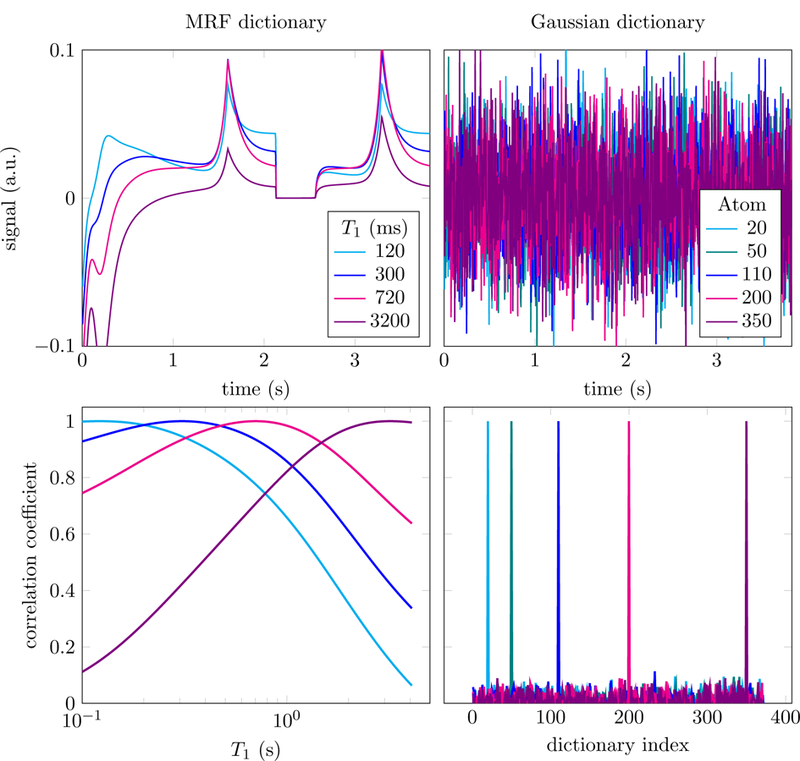
The figure shows a small selection of columns in a magnetic-resonance fingerprinting (MRF) dictionary (top left) and an i.i.d. Gaussian compressed-sensing dictionary (top right). In the MRF dictionary, generated using the approach in [3,4] which produces real-valued fingerprints, each fingerprint corresponds to a value of the relaxation parameter T1 (T2 is fixed to 62 ms). In the bottom row we show the correlation of the selected columns with every other column in the dictionary. This reveals the high local coherence of the MRF dictionary (left), compared to the incoherence of the compressed-sensing dictionary (right).
Coherence is not only a problem from a theoretical point of view. Most fast-estimation methods for sparse recovery exploit the fact that for incoherent dictionaries like the Gaussian dictionary in Figure 4 the Gram matrix D∗D is close to the identity. As a result, multiplying the data by the transpose of the dictionary yields a noisy approximation to the sparse coefficients
| (2.24) |
which can be cleaned up using some form of thresholding. This concept is utilized by greedy approaches such as orthogonal matching pursuit [60] or iterative hard-thresholding methods [10], as well as fast algorithms for 𝓁1-norm minimization such as proximal methods [22] and coordinate descent [34], which use iterative soft-thresholding instead. In our experiments with MRF dictionaries, for which D*y is not approximately sparse due to the correlations between columns (see the second row of Figure 5), these techniques fail to produce accurate estimates. As an example, Figure 5 shows the result of applying iterative hard thresholding (IHT) [10] to an MRF dictionary. The estimated coefficients are sparse, but closer to the maximum of D*y than to the true values. In contrast, the method is very effective when applied in a compressed- sensing setting, where the dictionary is incoherent (see right column of Figure 5).
Figure 5:
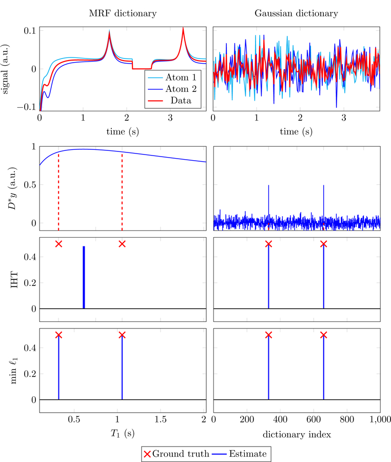
The data in the top row are an additive superposition of two columns from the MRF (left) and the compressed-sensing (right) dictionaries depicted in Figure 4. The correlation between the data and each dictionary column (second row) is much more informative for the incoherent dictionary (right) than for the coherent one (left). Iterative hard thresholding (IHT) [10] (third row) achieves exact recovery of the true support for the compressed-sensing problem (right), but fails for MRF (left) where it recovers two elements that are closer to the maximum of the correlation than to the true values. In contrast, solving (2.27) using a high-precision solver [36] achieves exact recovery in both cases (bottom row).
Recently, theoretical guarantees for sparse-decomposition methods have been established for dictionaries arising in super-resolution [15,31] and deconvolution problems [7]. As in the case of MRF, these dictionaries have very high local correlations between columns. These papers show that although robust recovery of all sparse signals in such dictionaries is not possible due to their high coherence, 𝓁1-norm minimization achieves exact recovery of a more restricted class of signals: sparse signals with nonzero entries corresponding to dictionary columns that are not highly correlated. To be clear, arbitrarily high local correlations may exist in the dictionary, as long the columns that are actually present in the measured signal are relatively uncorrelated with each other. Although this theory does not apply directly to MRF, it suggests that recovery may be possible for multicompartment models where the fingerprints of the tissues present in each voxel are sufficiently different. Indeed, our numerical results confirm this intuition, as illustrated by Figure 5 where 𝓁1-norm minimization achieves exact recovery also for the coherent MRF dictionary. Solving the convex program
| (2.25) |
| (2.26) |
| (2.27) |
makes it possible to successfully fit the sparse multicompartment model, as long as the parameters of each compartment are not too close (see Figure 12). Interestingly, in our experiments we observe that for these dictionaries it is often necessary to use high-precision second-order methods [36] in order to achieve exact recovery. In contrast, fast 𝓁1 -norm minimization algorithms based on soft-thresholding or coordinate descent tend to converge very slowly due to the coherence of the dictionary, even for small-scale problems (see Figure 6).
Figure 12:
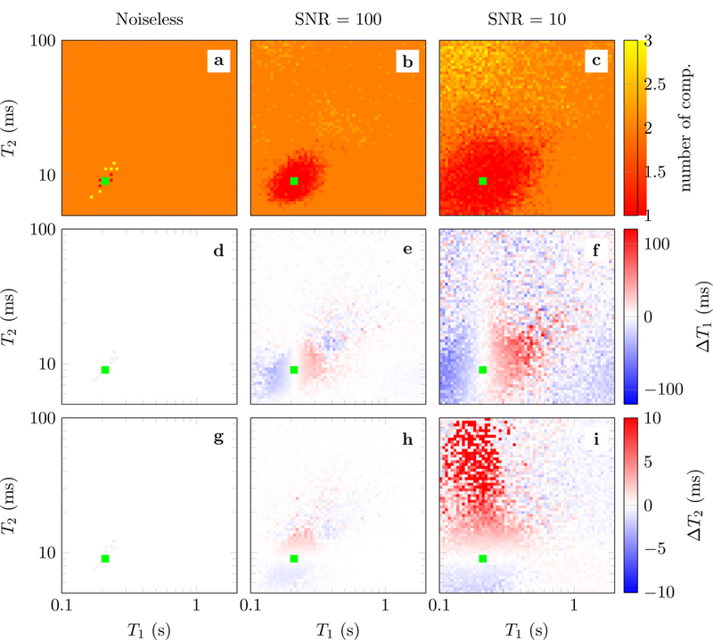
Results of fitting a multicompartment model where one compartment is fixed to T1 = 0.21 s and T2 = 9 ms (marked by the green square), and the second compartment has different T1 (between 0.1 s and 2.0 s) and T2 values (between 5 ms and 100 ms) The proton density of each compartment is fixed to 0.5. The fingerprints are generated following Refs. [3,4]. The data are perturbed by adding i.i.d. Gaussian noise to obtain two different SNRs (second and third columns). The multicompartment model is fit using the reweighting scheme defined in Eq. (2.31) combined with the method in Section 2.6. The heat maps shows the results for each different T1 and T2 value of the second compartment at the corresponding position in T1-T2 space, color-coded as indicated by the colorbars. The first row depicts the number of compartments resulting from the reconstruction (the ground truth is two). The second and third row show the T1 and T2 errors for the first compartment respectively. These errors correspond to the difference between the relaxation times of the fixed compartment (T1 = 0.21 s and T2 = 9) and the closest relaxation time of the reconstructed atoms. The results are averaged over 5 repetitions with different noise realizations.
2.5. Robust sparse estimation via reweighted-𝓁1-norm minimization
In the previous section, we discuss exact recovery of the sparse coefficients in a multicompartment model under the assumptions that (1) there is no noise and (2) the fingerprints corresponding to the true parameters are present in the dictionary. In practice, neither of these assumptions holds: noise is unavoidable and the tissue parameters may not fall exactly on the chosen grid. In fact, the vector x represents a column in at iteration l of the alternating scheme described in Section 2.2 and is therefore also subject to aliasing artifacts. A standard way to account for perturbations and model imprecisions in sparse-recovery problems is to relax the 𝓁1-norm minimization problem (2.27) to a regularized least-squares problem of the form
| (2.28) |
where λ ≥ 0 is a regularization parameter that governs the trade-off between the least-squares data-consistency term and the 𝓁1-norm regularization term. Solving (2.28) to perform sparse recovery is a popular sparse-regression method known as the lasso in statistics [70] and basis pursuit in signal processing [21].
The top row of Figure 6 shows the results of estimating the components of a noisy MRF signal by solving problem (2.28) using a high-precision interior-point method for different values of the parameter λ. For large values of λ, the solution is sparse, but the fit to the data is not very accurate and the true support is not well approximated. For small values of λ, the solution to the convex program correctly locates the vicinity of the true coefficients, but is contaminated by small spurious spikes. Perhaps surprisingly, a popular first-order method based on soft-thresholding called FISTA [5] produces solutions that are quite dense, a phenomenon previously reported in [54]. This suggests that higher-precision solvers may be needed to fit sparse linear models for coherent dictionaries, as opposed to incoherent dictionaries for which low-precision methods such as FISTA are very effective.
Reweighted-𝓁1-methods [19, 76] are designed to enhance the performance of 𝓁1-norm-regularized problems by promoting sparser solutions that are close to the initial estimate. In the case of the MRF dictionary, these methods are able to remove spurious small spikes, while retaining an accurate support estimate. This is achieved by solving a sequence of weighted 𝓁1-norm regularized problems of the form
| (2.29) |
for k = 1, 2, …. We denote the solution of this optimization problem by . The entries in the initial vector of weights ω(1) are initialized to one, so is the solution to problem (2.28). The weights are then updated depending on the subsequent solutions to problem (2.29).
We consider two different reweighting schemes. The first, proposed in [19], simply sets the weights to be inversely proportional to the previous estimate
| (2.30) |
where is a parameter typically fixed to a very small value with respect to the expected magnitudeof the nonzero coefficients (e.g. 10−8) in order to preclude division by zero (see [19] for more details).
Intuitively, the weights penalize the coefficients that do not contribute to the fit in previous iterations, promoting increasingly sparse solutions. Mathematically, the algorithm can be interpreted as a majorization-minimization method for a non-convex sparsity-inducing penalty function [19]. The second updating scheme, proposed in [76] and inspired by sparse Bayesian learning methods [77], is of the form
| (2.31) |
| (2.32) |
| (2.33) |
The parameter precludes the matrix from being singular and can be set to a very small fixed value (e.g. 10−8). The reweighting scheme sets to be small if there is any large entry such that the corresponding columns of the dictionary Di and Dj are correlated. This produces smoother weights than (2.30) providing more robustness to initial errors in the support estimate.
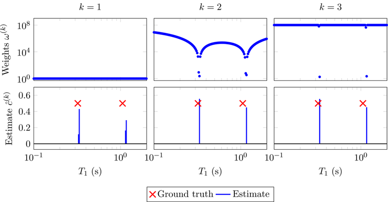
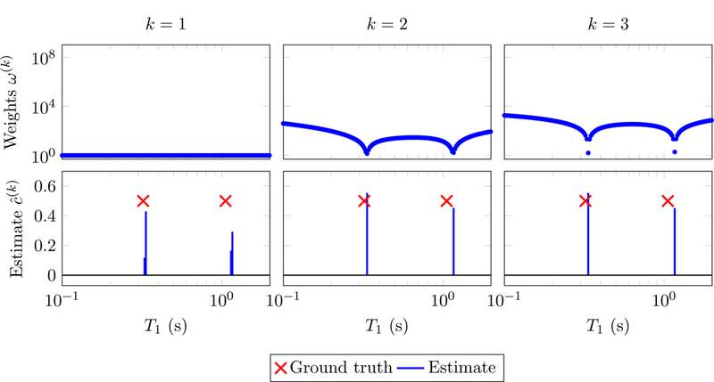
Figures 7 and 8 show the results obtained by applying reweighted-𝓁1-norm regularization to the same problem as in Figure 6. As expected, the update (2.31) yields smoother weights. Convergence to a sparse solution is achieved in just two iterations. The estimate is an accurate estimate of the parameters despite the presence of noise and the gridding error (the true parameters do not lie on the grid used to construct the dictionary).
Figure 7:
Solutions to problem (2.29) (bottom) and corresponding weights (top) computed following the reweighting scheme (2.30), with λ := 10−3 and := 10−8. The data are the same as in Figure 6.
Figure 8:
Solutions to problem (2.29) (bottom) and corresponding weights (top) computed following the reweighting scheme (2.31), with λ := 10−3 and := 10−8. The data are the same as in Figure 6.
Finally, we would like to mention reweighted least-squares, a sparse-recovery method applied to an MRF multicompartment model in [54]. Similarly to the reweighted-𝓁1 norm method given by (2.31), this technique is based on a nonconvex cost function derived by Bayesian principles. The resulting scheme is not as accurate as the reweighting 𝓁1-norm based methods (see Figure 9) and often yields solutions that are not sparse, as reported in [54]. However, it is extremely fast, since it just requires solving a sequence of regularized least-squares problems. Unfortunately, this also means that the nonnegativity assumption on the coefficients cannot be easily incorporated (the intermediate problems then become nonnegative least-squares problems which no longer have closed-form solutions). Developing fast methods that incorporate such constraints and are effective for coherent dictionaries is an interesting topic for future research. In this work, our method of choice for the sparse-recovery problem arising in multicompartment MRF is least squares with reweighted-𝓁1-norm regularization, implemented using an efficient interior-point solver described in the following section.
2.6. Fast interior-point solver for 𝓁1-norm regularization in coherent dictionaries
In this section we describe an interior-point solver for the 𝓁1-norm regularized problem
| (2.34) |
| (2.34) |
which allows us to apply the reweighting schemes described in Section 2.5 efficiently. Interior-point methods enforce inequality constraints by using a barrier function [12,58,79]. In this case we use a logarithmic function that forces the coefficients to be nonnegative. Parametrizing the modified optimization problem with t > 0, we obtain a sequence of cost functions of the form
| (2.35) |
The central path of the interior-point scheme consists of the minimizers of as t varies from 0 to ∞. To find a solution for problem 2.34, we find a sequence of points c(1), c(2), … in the central path by iteratively solving the Newton system
| (2.36) |
where
| (2.37) |
This is essentially the approach taken in [13,43] to tackle 𝓁1-norm regularized least squares. Solving (2.36) is the computational bottleneck of this method. In the case of the MRF dictionary, D∗D is a matrix of rank k, where k is the order of the low-rank approximation to the dictionary described in Section 2.3. As a result, solving the Newton system (2.36) directly is extremely slow for large values of t. Ref. [43] suggests applying a preconditioner of the form
| (2.38) |
combined with an iterative conjugate-gradient method to invert the system. However, in our case the preconditioner is not very effective in improving the conditioning of the Newton system, as shown in Figure 10.
Figure 10:
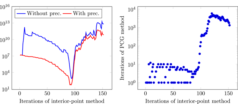
The left image shows the condition number of the matrix in the Newton system (2.36) with and without the preconditioning defined in (2.38), as the interior-point solver proceeds. Preconditioning does not succeed in significantly reducing the condition number, especially as the method converges. The right image shows the number of conjugate-gradient iterations needed to solve the preconditioned Newton system, which become impractically large after 100 iterations. The experiment is carried out by fitting a two-compartment model using a dictionary containing 104 columns.
In order to solve the Newton system (2.36) efficiently, we take a different route: exploiting the low-rank structure of the Hessian by applying the Woodbury inversion lemma, also known as Sherman-Morrison-Woodbury formula. Lemma 2.1 (Woodbury inversion lemma). Assume A and . Then,
| (2.39) |
Setting A := Z, B := D, G := D* and in the lemma yields the following expression for the inverse of the system matrix
| (2.40) |
Since in practice k is very small (typically between 10 and 15) due to the dictionary-compression scheme described in Section 2.3 and Z is diagonal, using this formula accelerates the inversion of the Newton system dramatically.
Figure 11 compares the computational cost of our method based on Woodbury-inversion with a general-purpose convex-programming solver based on an interior-point method [36] and an interiorpoint method tailored to large-scale problems, which applies the preconditioner in Eq. (2.38) and uses an iterative method to solve the Newton system [43]. Our method is almost an order of magnitude faster for dictionaries containing up to 104 columns.
Figure 11:
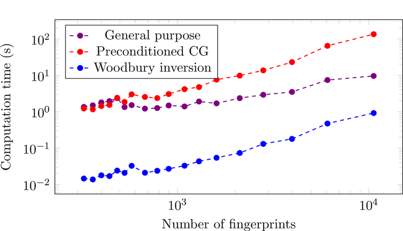
Computation times of the proposed Woodbury-inversion method compared to a generalpurpose solver [36] and an approach based on preconditioned conjugate-gradients (CG) [43]. MRF dictionaries containing different numbers of fingerprints in the same range (T1 values from 0.1 s to 2 s, T2 values from 0.005 s to 0.1 s) were generated using the approach described in Refs. [3,4]. Each method was applied to solve 10 instances of problem (2.34) for each dictionary size on a computer cluster (Four AMD Opteron 6136, each with 32 cores, 2.4 GHz, 128 GB of RAM). In all cases, the interior-point iteration is terminated when the gap between the primal and dual objective functions is less than 10−5.
To conclude, we note that this algorithm can be directly applied to weighted 𝓁1-norm-regularization least squares problems of the form
| (2.41) |
where W is a diagonal matrix containing the weights. We just need to apply the change of variable and . Since the weights are all positive, the constraint is equivalent to .
3. Results
3.1. Numerical simulations
In this section we evaluate the performance of the sparse recovery algorithm described in Sections 2.5 and 2.6 on simulated data.
3.1.1. Single-voxel data
In this section we consider simulated data from a voxel that contains two compartments with equal relative contribution. The parameters of the first compartment are fixed (T1 = 0.21 s, T2 = 9 ms), whereas the parameters of the second compartment vary on a grid (T1 between 0.1 s and 2.0 s and T2 between 5 ms and 100 ms). To make the setting more realistic and incorporate discretization error, the dictionary used for recovery does not match the one used to simulate the data. The data are generated by adding the fingerprints from the two compartments and perturbing the result with i.i.d. Gaussian noise. The signal-to-noise ratio is defined as the ratio between the 𝓁2 norm of the signal and the noise.
Figure 12 shows the error when fitting the multicompartment model using the reweighting scheme defined in Eq. (2.31). The error of the fixed compartment is depicted as a function of the relaxation times of the second compartment. The closer the two compartments are in T1-T2-space, the more correlated their corresponding fingerprints are, which results in a more challenging sparse-recovery problem. In the noiseless case, exact recovery occurs (even without reweighting) except for combination of tissues with almost identical relaxation times. For the noisy data, the algorithm tends to detect the correct number of compartments as long as the relaxation times of the two compartments are sufficiently separated (b, c). When the relaxation times of the two compartments are very similar, the algorithm cannot separate the compartments and returns, as expected, a single compartment (cf. red region around the green square in Subfigure b). Increasing the noise increases the size of this region (c). Within the region, one can observe that the relaxation times of the reconstructed single compartment lie between the two original compartments (e, f, h, i). Outside of the region, where multiple compartments are detected, the observed error is mostly noise-like and increases as the noise level increases (e, f, h, i). In some cases, a spurious third compartment can be observed (b, c).
3.1.2. Boundary estimation
When applying the proposed approach to the numerical experiment sketched in Figure 1, we find that the two contributing compartments are correctly identified (Figure 13). The relaxation times of both compartments are constant over space, in accordance with the ground truth. The proton density, which reflects the relative contributions of each compartment to the signal, exhibits a gradual variation that correctly reflects the effect of the low-pass filtering of the measurements in Fourier space.
Figure 13:
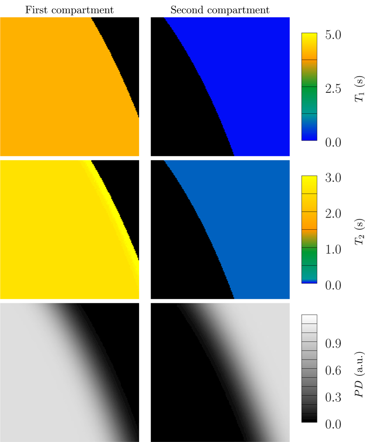
Results of fitting our multicompartment model, using the algorithm described in Section 2.5 and Section 2.6, to the data in Figure 1. The proposed multicompartment reconstruction correctly identifies the relaxation times of the two compartments, as well as their relative contributions, quantified by the proton density (PD) of each compartment. T1 and T2 maps of all voxels with proton density less than 0.01 are depicted in black. Since the simulated data do not contain noise, we set the regularization parameter λ to a very small value (10−8. The reweighting parameter is set to 10−10.
3.1.3. Simulated phantom
In this section we evaluate our methods on a numerical phantom that mimics a realistic MRF experiment with radial Fourier, or k-space sampling. The numerical phantom has 16 different 19×19 voxel regions. The voxels in each region consist of either one or two compartments with relaxation times in the same range as biological tissues such as myelin-water (A), gray matter (B), white matter (C), and cerebrospinal fluid (C). Figure 14 depicts the structure of the phantom along with the corresponding relaxation times. For each compartment, a fingerprint was calculated with Bloch simulations utilizing the flip-angle pattern described in [4] (see Fig. 3k). These fingerprints are then combined additively to yield the multicompartment fingerprints of each voxel. The data correspond to undersampled k-space data of each time frame, calculated with a non-uniform fast Fourier transform [2,32] with 16 radial k-space spokes per time frame. The fingerprints consist of 850 time frames, and the trajectory of successive time frames are rotated by 16 times the golden angle with respect to each other [75]. Noise with an i.i.d Gaussian distribution was added to the simulated k-space data to achieve different signal-to-noise ratios.
Figure 14:
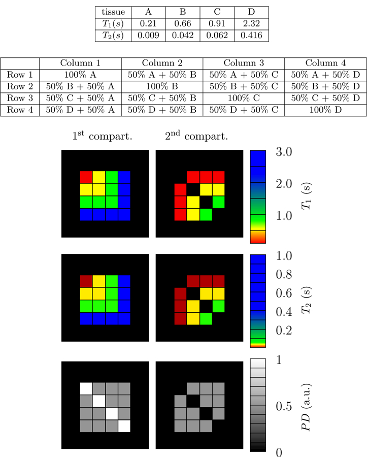
The numerical phantom consists of four different synthetic tissues with relaxation times in the range commonly found in biological brain tissue. Each voxel contains one or two tissue compartments, as depicted in the figure. The relaxation times of the tissues A, B, C and D are in the range found in myelin-water, gray matter, white matter, and cerebrospinal fluid respectively.
When two different tissues are present in a voxel, two conditions are necessary so that the problem of distinguishing their contributions to the signal is well posed. First, their corresponding fingerprints should be sufficiently distinct, i.e. have a low correlation coefficient (see Section 2.4). Second, the weighted sum of their fingerprints should be different from any other fingerprint in the dictionary. Otherwise, a single-compartment model will fit the data well. Figure 15 shows the correlations between the fingerprints corresponding to each of the tissues present in the numerical phantom and the rest of the fingerprints in the dictionary. For tissues that have similar T1 and T2 values, the correlation is very high. In particular, the fingerprints corresponding to tissue B and C are extremely similar. Furthermore, their additive combination is almost indistinguishable from another fingerprint also present in the dictionary, as illustrated in Figure 16. It will consequently be almost impossible to distinguish a voxel containing a single tissue with that particular fingerprint and a two-compartment voxel containing tissue B and C if there is even a very low level of noise in the data. Fortunately, this is not the case for the other combinations of the four relaxation times of interest.
Figure 15:
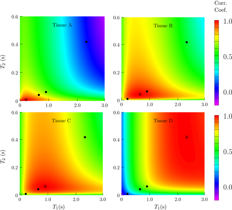
Correlation between the fingerprints corresponding to the four tissues present in the numerical phantom with every other fingerprint in the dictionary, indexed by the corresponding T1 and T2 values. The tissue corresponding to the fixed fingerprint is marked with a star, the position of the other three tissues also present in the phantom are marked with dots.
Figure 16:
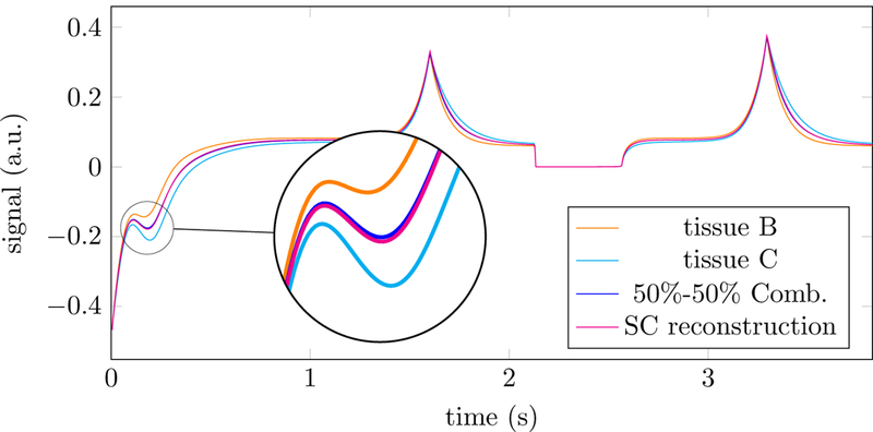
Simulated fingerprints of tissue B and C, and a 50%−50% combination of those tissues are shown, along with a single-compartment (SC) reconstruction, i.e. the fingerprint in the dictionary that is closest to the 50%−50% combination. In this particular example, the fingerprints of those tissues are highly correlated, and the single-compartment reconstruction represents the data well (the relative error in the 𝓁2-norm is 1.42%). As a result, the multicompartment reconstruction cannot distinguish the two compartments if the data contain even a small level of noise.
To estimate the relaxation times T1 and T2 from the simulated data we apply the method described in Section 2.2 while fixing the number of ADMM iterations to 10. We compress the dictionary by truncating its SVD to obtain a rank-10 approximation, as described in Section 2.3. The magnetization vector is updated by applying 10 conjugate-gradient iterations. The coefficient variable is updated by applying the reweighted-𝓁1 method described in Section 2.5 over 5 iterations with the reweighting scheme in equation (2.30) (the reweighting scheme (2.31) yields similar results). For each iteration, the interior-point method described in Section 2.6 is run until the gap between the primal and dual objective functions is less than 10-5.
Figure 17 shows the reconstructed parameter maps for a signal-to-noise ratio (SNR) of 103 (the SNR is defined as the ratio between the 𝓁1 norm of the signal and the added noise), and using 16 radial k-space spokes. The multicompartment reconstruction recovers the two compartments accurately, except for the voxels that contain the highly-correlated tissues B and C. This behavior is expected due to the high correlations of the fingerprints of those tissues (see Figure 16). The model also yields an accurate estimate of the proton density of the compartments that are present in each voxel (except, again, for voxels containing tissue B and C). In most voxels, the reconstruction does not detect additional compartments, even though this is is not explicitly enforced. Figure 18 shows that the performance degrades gracefully when the SNR is decreased to 100: the model still achieves similar results, only noisier, and a spurious third compartment with a relatively low proton density appears in some voxels.
Figure 17:
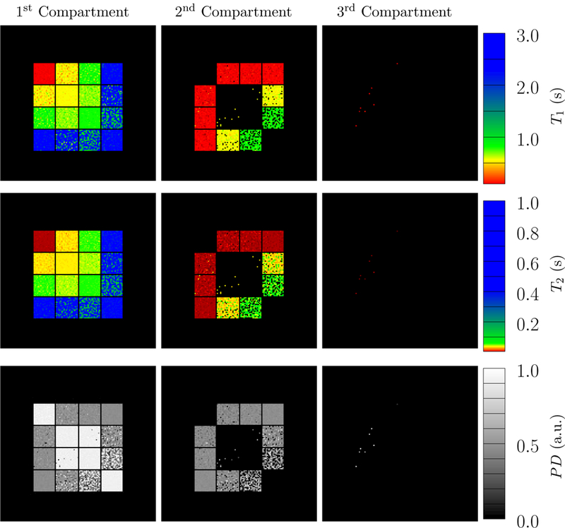
The depicted parameter maps were reconstructed from data simulated with an SNR = 103 and using 16 radial k-space spokes. The proton density (PD, third row) indicates the fraction of the signal corresponding to the recovered compartments. The compartments in each voxel are sorted according to their 𝓁2-norm distance to the origin in T1-T2 space. Compare to Figure 14, which shows the ground truth.
Figure 18:
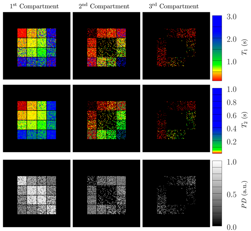
The depicted parameter maps were reconstructed from data simulated with an SNR = 100 and using 16 radial k-space spokes. The proton density (PD, third row) indicates the fraction of the signal corresponding to the recovered compartments. The compartments in each voxel are sorted according to their 𝓁2-norm distance to the origin in T1-T2 space. Compare to Figure 14, which shows the ground truth.
To evaluate the performance of the method at different undersampling factors, we fit the multicompartment model to the simulated phantom data using different number of radial k-space spokes. Figure 19 shows the decrease in the normalized root-mean-square-error (NRMSE) of the T1 and T2 estimates averaged over all voxels in the phantom. As expected, the NRMSE decreases when acquiring more k-space spokes. As explained above, the largest contributor to the NRMSE are the voxels that contain both tissue B and C, so the NRMSE excluding these voxels is also depicted. The scatter plots in Figure 20 show the results at each voxel containing a 50%−50% mixture of tissues A and C. The two compartments are separated accurately, even when only two radial k-space spokes are measured. As more samples are gathered, the two clusters corresponding to the two tissues concentrate more tightly around the ground truth. Similarly, when keeping the number of k-space spokes fixed and increasing the SNR, the NRMSE decreases as expected (Figure 21) and the estimated parameters converge to the ground truth (Figure 22). The dependence of the reconstruction quality on the correlation of the fingerprints is visualized in Figure 23, where scatter plots for all tissue combinations are shown. One can observe a dependency of the reconstruction quality on the distance of the two compartments in parameter space. In particular, the combination of tissues B and C, which have highly correlated fingerprints, results in a single compartment fit (see Figure 16).
Figure 19:
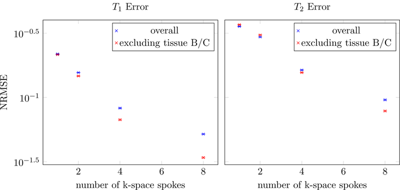
The normalized root-mean-square errors (NRMSE) in the T1 and T2 estimates are plotted as a function of the number of radial k-space spokes at a fixed SNR = 1000. The NRMSE is defined as the root-mean square of the ∆T1,2/T1,2. The results are averaged over 10 realizations of the noise, and the hardly-visible error bars depict one standard deviation of the variation between different noise realizations. The NRMSE was also computed excluding voxels containing a combination of tissue B and C, because the corresponding fingerprints are highly correlated.
Figure 20:
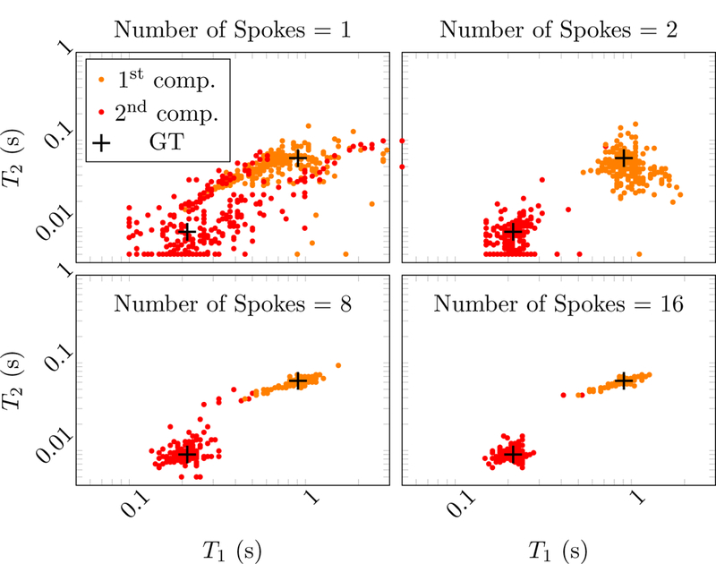
Scatter plots showing the estimated T1 and T2 values in the multicompartment model for voxels containing tissue A and C. Different number of radial k-spaces spokes are tested at a fixed SNR of 103. The two clusters corresponding to the two tissues concentrate more tightly around the ground truth (GT, marked with black crosses) as the number of spokes increases.
Figure 21:
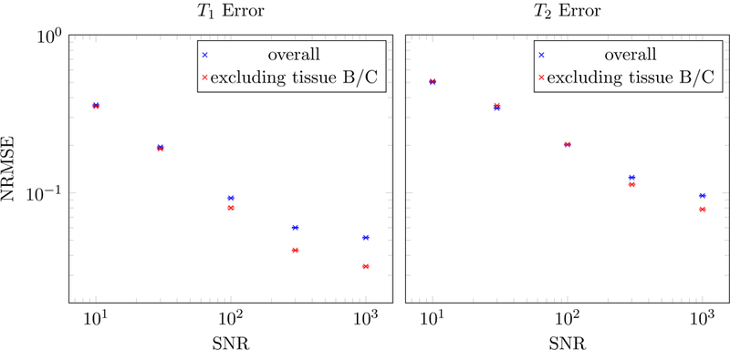
The normalized root-mean-square errors (NRMSE) in the T1 and T2 estimates are plotted as a function of the SNR when acquiring 8 radial k-space spokes. The NRMSE is defined as the root-mean square of the ∆T1,2/T1,2. The results are averaged over 10 realizations of the noise, and the hardly-visible error bars depict one standard deviation of the variation between different noise realizations. The NRMSE was also computed excluding voxels containing a combination of tissue B and C, because the corresponding fingerprints are highly correlated.
Figure 22:
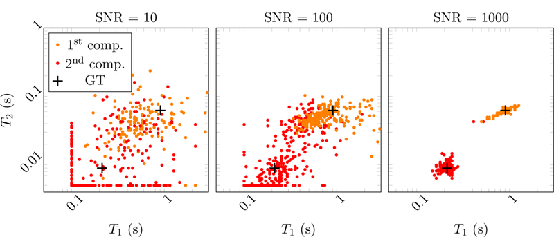
Scatter plots showing the estimated T1 and T2 values in the multicompartment model for voxels containing tissue A and C. The data was reconstructed from 16 radial k-space spokes. The two clusters corresponding to the two tissues concentrate more tightly around the ground truth (GT, marked with black crosses) as the SNR increases.
Figure 23:
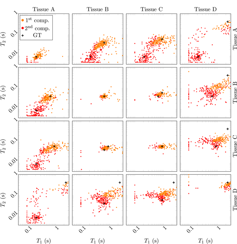
Scatter plots showing the estimated T1 and T2 values in the multicompartment model for simulated data with an SNR = 100 and using 16 radial k-space spokes. The tissues contained in those voxels are indicated above and to the right. The ground truth value of their respective relaxation times is marked with black crosses.
3.2. Phantom experiment
For validation on real data, we performed an imaging experiment on a clinical MR system with a field strength of 3 Tesla (Prisma, Siemens, Erlangen, Germany). We designed a dedicated phantom and manufactured it using a 3D printer (Figure 24). The structure of the phantom is effectively the same as that of the simulated phantom described in Section 3.1 and Figure 14: the diagonal elements contain only one compartment, whereas the off-diagonal elements contain two compartments. The compartments were filled with different solutions of doped water in order to achieve relaxation times in the range of biological tissues. MRF scans were performed with the sequence described in Fig. 3k of Ref. [4] with 8 radial k-space spokes per time frame and the same parameters otherwise.
Figure 24:
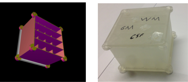
Computer-aided design (left) and the corresponding 3D-printed phantom (right) used for the phantom evaluation. It contains two layers, one with four horizontal and one with four vertical bars. Imaging a slice that contains both layers results in the same effective structure as the numerical phantom shown in Figure 14.
Figure 25 shows the parameter maps reconstructed with a single-compartment model and a low rank ADMM algorithm [2]. For the diagonal elements of the grid phantom, which only contain signal from a single compartment, we consider the identified T1 and T2 values listed in Table 1 as the reference gold standard. In the off-diagonal elements, the single-compartment model fails to account for the presence of two compartments, so the apparent relaxation times lie in between the true values of the two compartments. Note that the square shape of the phantom causes significant variations in the main magnetic field towards the edges of the phantom. Since we do not account for those variations, substantial artifacts can be observed in those areas (Figure 25).
Figure 25:
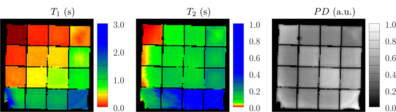
The depicted parameter maps were reconstructed from data measured in a phantom and using a single-compartment model. The data were acquired using 8 radial k-space spokes. The colorbar is adjusted so that distinct colors correspond to the parameters of the gold-standard reference measurements: red, yellow green and blue represent the solutions A-D.
Table 1:
The gold-standard (GS) values measured by single-compartment reconstruction on the diagonal grids of phantom described in Figure 24, where only a single compartment is present.
| A | B | C | D | |
|---|---|---|---|---|
| T1 (s) | 0.1262 ± 0.0075 | 0.5075 ± 0.015 | 0.7640 ± 0.055 | 1.831 ± 0.061 |
| T2 (s) | 0.0174 ± 0.0046 | 0.1019 ± 0.0084 | 0.1328 ± 0.018 | 0.66 ± 0.21 |
Figure 26 shows the parameter maps reconstructed with the proposed multicompartment reconstruction method. At the diagonal elements, results are consistent with the single-compartment reconstruction, except for some voxels where a spurious second compartment appears with low proton density. This indicates that the method correctly identifies voxels containing only a single compartment. In the off-diagonal grid elements, two significant compartments are detected for most voxels, and the relaxation times coincide with the gold-standard within a standard deviation (Table 2), even though the noise level is quite severe at the given experimental conditions. A spurious third compartment with low proton density is detected in some voxels. Many voxels containing the combination of the doped water solutions B and C are reconstructed as a single compartment with apparent relaxation times between the gold-standard values. This is expected, since the corresponding fingerprints are almost indistinguishable, as in the case of the simulated tissues B and C (see Fig. 12). Errors are larger for T2 than for T1, as expected from the Cramer´-Rao bound estimation performed in [4]. The artifacts towards the edge of the phantom are due to variations in the main magnetic field (this effect is also visible in the single-compartment reconstruction in Figure 25).
Figure 26:
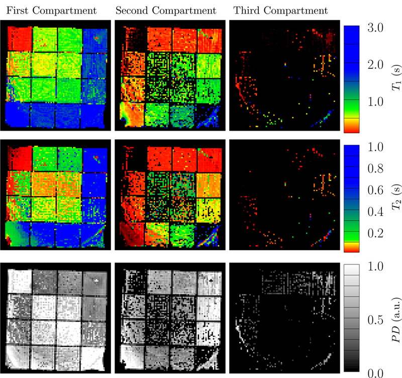
The parameter maps of the scanned phantom was reconstructed using the proposed multicompartment method. The data were acquired using eight radial k-space spokes. The three compartments with the highest detected proton density are shown here, and are sorted in each voxel according to their 𝓁2-norm distance to the origin in T1-T2 space. The colorbar is adjusted so that distinct colors correspond to the parameters of the gold-standard reference measurements: red, yellow green and blue represent the four solutions.
Table 2:
Mean values and standard deviations of the multicompartment estimates for the selected combinations appearing in Figure 27.
| A and C | A and D | B and D | ||||
|---|---|---|---|---|---|---|
| A | C | A | D | B | D | |
| T1 (s) | 0.35 ± 0.25 | 0.58 ± 0.26 | 0.24 ± 0.26 | 1.40 ± 0.57 | 0.66 ± 0.18 | 1.49 ± 0.36 |
| T2 (s) | 0.068 ± 0.071 | 0.20 ± 0.20 | 0.063 ± 0.24 | 1.20 ± 0.58 | 0.080 ± 0.11 | 1.25 ± 0.44 |
Further insights are provided by the scatter plots depicted in Figure 27, which show the estimated relaxation times of the voxels containing three combinations of tissues. For these combinations, the multicompartment reconstruction correctly detects the presence of both tissues and the estimated relaxation times cluster around the gold-standard values. In contrast, the single-compartment algorithm results in a single cluster of apparent relaxation times at a position in parameter space that provides little information about the underlying tissue composition.
Figure 27:
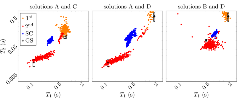
The scatter plot shows the estimated relaxation times of the measured phantom at the example of voxels containing different combinations of compartments. For comparison, the estimates obtained from the single-compartment (SC) are shown, as well as the gold-standard (GS) values measured on the diagonal, where only a single compartment is present. The rectangles represent the standard deviation of the gold-standard measurement.
4. Conclusions and Future Work
In this work we propose a framework to perform quantitative estimation of parameter maps from magnetic resonance fingerprinting data, which accounts for the presence of more than one tissue compartment in each voxel. This multi-compartment model is fit to the data by solving a sparse linear inverse problem using reweighted 𝓁1-norm regularization. Numerical simulations show that an efficient interior-point method is able to tackle this sparse-recovery problem, yielding sparse solutions that correspond to the parameters of the tissues present in the voxel.
The proposed method is validated through simulations, as well as with a controlled phantom imaging experiment on a clinical MR system. The results indicate that incorporating a sparse-estimation procedure based on reweighed 𝓁1-norm regularization is a promising avenue towards achieving multicompartment parameter mapping from MRF data. However, the proposed method still requires a high SNR, which entails long scan times for in vivo applications. A promising research direction is to incorporate additional prior assumptions on the structure of the parameter maps in order to leverage the method in the realm of clinically-feasible scan times. Future work will also include the application of the proposed framework to the quantification of the myelin-water fraction in the human brain, which is an important biomarker for neurodegenerative diseases.
Acknowledgements
C.F. is supported by NSF award DMS-1616340. J.A., F.K., R.L. and M.C. are supported by NIH/NIBIB R21 EB020096, NIH/NIAMS R01 AR070297 and NIH P41 EB017183. S. L. is supported by a seed grant from the Moore-Sloan Data-Science Environment at NYU. S. T. is supported in part by the Office of Naval Research under Award N00014–17-1–2059.
References
- [1].Allerhand A and Gutowsky HS. Spin-Echo NMR Studies of Chemical Exchange. I. Some General Aspects. The Journal of Chemical Physics, 41:2115–2126, Oct. 1964. [DOI] [PubMed] [Google Scholar]
- [2].Assländer J, Cloos MA, Knoll F, Sodickson DK, Hennig J, and Lattanzi R. Low rank alternating direction method of multipliers reconstruction for mr fingerprinting. Magnetic Resonance in Medicine, 79(1):83–96, 2018. [DOI] [PMC free article] [PubMed] [Google Scholar]
- [3].Assländer J, Glaser SJ, and Hennig J. Pseudo steady-state free precession for mr-fingerprinting. Magnetic resonance in medicine, 77(3):1151–1161, 2017. [DOI] [PubMed] [Google Scholar]
- [4].Assländer J, Lattanzi R, Sodickson DK, and Cloos MA. Relaxation in Spherical Coordinates: Analysis and Optimization of pseudo-SSFP based MR-Fingerprinting. arXiv, 1703.00481(v1), 2017. [Google Scholar]
- [5].Beck A and Teboulle M. A fast iterative shrinkage-thresholding algorithm for linear inverse problems. SIAM journal on imaging sciences, 2(1):183–202, 2009. [Google Scholar]
- [6].Becker SR, Candès EJ, and Grant MC. Templates for convex cone problems with applications to sparse signal recovery. Mathematical programming computation, 3(3):165–218, 2011. [Google Scholar]
- [7].Bernstein B and Fernandez-Granda C. Deconvolution of Point Sources: A Sampling Theorem and Robustness Guarantees. preprint, 2017. [Google Scholar]
- [8].Bickel PJ, Ritov Y, and Tsybakov AB. Simultaneous analysis of lasso and {D}antzig selector. The Annals of Statistics , pages 1705–1732, 2009. [Google Scholar]
- [9].Bloch F. Nuclear induction. Physical review, 70(7–8):460, 1946. [Google Scholar]
- [10].Blumensath T and Davies ME. Iterative hard thresholding for compressed sensing. Applied and computational harmonic analysis, 27(3):265–274, 2009. [Google Scholar]
- [11].Boyd S, Parikh N, Chu E, Peleato B, and Eckstein J. Distributed optimization and statistical learning via the alternating direction method of multipliers. Foundations and Trends R in MachineLearning , 3(1):1–122, 2011. [Google Scholar]
- [12].Boyd S and Vandenberghe L. Convex optimization Cambridge university press, 2004. [Google Scholar]
- [13].Candes E and Romberg J. 𝓁1-magic: Recovery of sparse signals via convex programming URL: www. acm. caltech. edu/𝓁1magic/downloads/𝓁1magic. pdf, 4:14, 2005.
- [14].Candes EJ. The restricted isometry property and its implications for compressed sensing. Comptes Rendus Mathematique, 346(9–10):589–592, 2008. [Google Scholar]
- [15].Candès EJ and Fernandez-Granda C. Towards a Mathematical Theory of Super-resolution. Communications on Pure and Applied Mathematics, 67(6):906–956, 2014. [Google Scholar]
- [16].Candès EJ, Romberg J, and Tao T. Robust uncertainty principles: Exact signal reconstruction from highly incomplete frequency information. IEEE Transactions on information theory, 52(2):489–509, 2006. [Google Scholar]
- [17].Candes EJ and Tao T. Decoding by linear programming. IEEE transactions on information theory, 51(12):4203–4215, 2005. [Google Scholar]
- [18].Candes EJ and Tao T. Near-optimal signal recovery from random projections: Universal encoding strategies? IEEE transactions on information theory, 52(12):5406–5425, 2006. [Google Scholar]
- [19].Candes EJ, Wakin MB, and Boyd SP. Enhancing sparsity by reweighted 𝓁1 minimization. Journal of Fourier analysis and applications, 14(5):877–905, 2008. [Google Scholar]
- [20].Chandrasekaran V, Recht B, Parrilo PA, and Willsky AS. The convex geometry of linear inverse problems. Foundations of Computational mathematics, 12(6):805–849, 2012. [Google Scholar]
- [21].Chen SS, Donoho DL, and Saunders MA. Atomic decomposition by basis pursuit. SIAM review, 43(1):129–159, 2001. [Google Scholar]
- [22].Combettes PL and Wajs VR. Signal recovery by proximal forward-backward splitting. Multiscale Modeling & Simulation, 4(4):1168–1200, 2005. [Google Scholar]
- [23].Deoni SC. Quantitative Relaxometry of the Brain. Topics in Magnetic Resonance Imaging, 21(2):101–113, 2010. [DOI] [PMC free article] [PubMed] [Google Scholar]
- [24].Deoni SCL, Matthews L, and Kolind SH. One component? two components? three? the effect of including a nonexchanging free water component in multicomponent driven equilibrium single pulse observation of t1 and t2. Magnetic Resonance in Medicine, 70(1):147–154, 2013. [DOI] [PMC free article] [PubMed] [Google Scholar]
- [25].Deoni SCL, Rutt BK, Arun T, Pierpaoli C, and Jones DK. Gleaning multicomponent T1 and T2 information from steady-state imaging data. Magnetic Resonance in Medicine, 60(6):1372–1387, 2008. [DOI] [PubMed] [Google Scholar]
- [26].Deshmane A, McGivney D, Badve C, Yu A, Jiang Y, Ma D, and Griswold MA. Accurate synthetic FLAIR images using partial volume corrected MR fingerprinting. In Proceedings of the 24th Annual Meeting of ISMRM, page 1909, 2016. [Google Scholar]
- [27].Donoho DL. Compressed sensing. IEEE Transactions on information theory, 52(4):1289–1306, 2006. [Google Scholar]
- [28].Donoho DL and Elad M. Optimally sparse representation in general (nonorthogonal) dictionaries via 𝓁1 minimization. Proceedings of the National Academy of Sciences, 100(5):2197–2202, 2003. [DOI] [PMC free article] [PubMed] [Google Scholar]
- [29].Ehses P, Seiberlich N, Ma D, Breuer FA, Jakob PM, Griswold MA, and Gulani V. Ir truefisp with a golden-ratio-based radial readout: Fast quantification of t1, t2, and proton density. Magnetic resonance in medicine, 69(1):71–81, 2013. [DOI] [PubMed] [Google Scholar]
- [30].Esser E, Lou Y, and Xin J. A method for finding structured sparse solutions to nonnegative least squares problems with applications. SIAM Journal on Imaging Sciences, 6(4):2010–2046, 2013. [Google Scholar]
- [31].Fernandez-Granda C. Super-resolution of point sources via convex programming. Information and Inference, 5(3):251–303, 2016. [Google Scholar]
- [32].Fessler J and Sutton B. Nonuniform fast fourier transforms using min-max interpolation. IEEE Trans. Signal Process, 51(2):560–574, February 2003. [Google Scholar]
- [33].Friedman J, Hastie T, and Tibshirani R. The elements of statistical learning, volume 1 Springer series in statistics Springer, Berlin, 2001. [Google Scholar]
- [34].Friedman J, Hastie T, and Tibshirani R. Regularization paths for generalized linear models via coordinate descent. Journal of statistical software, 33(1):1, 2010. [PMC free article] [PubMed] [Google Scholar]
- [35].Giedd JN, Snell JW, Lange N, Rajapakse JC, Casey BJ, Kozuch PL, Vaituzis AC, Vauss YC, Hamburger SD, Kaysen D, and Others. Quantitative magnetic resonance imaging of human brain development: ages 4–18. Cerebral cortex, 6(4):551–559, 1996. [DOI] [PubMed] [Google Scholar]
- [36].Grant M, Boyd S, Grant M, Boyd S, Blondel V, Boyd S, and Kimura H. Cvx: Matlab software for disciplined convex programming, version 2.1. Recent Advances in Learning and Control, pages 95–110. [Google Scholar]
- [37].Gribonval R and Nielsen M. Sparse representations in unions of bases. IEEE transactions on Information theory, 49(12):3320–3325, 2003. [Google Scholar]
- [38].Gunn RN, Gunn SR, Turkheimer FE, Aston JA, and Cunningham VJ. Positron emission tomography compartmental models: a basis pursuit strategy for kinetic modeling. Journal of Cerebral Blood Flow & Metabolism, 22(12):1425–1439, 2002. [DOI] [PubMed] [Google Scholar]
- [39].Hamilton JI, Deshmane A, Hougen S, Griswold M, and Seiberlich N. Magnetic Resonance Fingerprinting with Chemical Exchange (MRF-X) for Quantification of Subvoxel T1, T2, Volume Fraction, and Exchange Rate. In Proc. Intl. Soc. Mag. Reson. Med 23, page 329, 2015. [Google Scholar]
- [40].Han X, Jovicich J, Salat D, van der Kouwe A, Quinn B, Czanner S, Busa E, Pacheco J, Albert M, Killiany R, Maguire P, Rosas D, Makris N, Dale A, Dickerson B, and Fischl B. Reliability of MRI-derived measurements of human cerebral cortical thickness: The effects of field strength, scanner upgrade and manufacturer. NeuroImage, 32(1):180–194, 2006. [DOI] [PubMed] [Google Scholar]
- [41].Hastie T, Tibshirani R, and Wainwright M. Statistical learning with sparsity CRC press, 2015. [Google Scholar]
- [42].Heins P, Moeller M, and Burger M. Locally sparse reconstruction using the 𝓁1 ,∞-norm. arXiv preprint arXiv:1405.5908, 2014. [Google Scholar]
- [43].Kim S-J, Koh K, Lustig M, Boyd S, and Gorinevsky D. An interior-point method for large-scale 𝓁1-regularized least squares. IEEE journal of selected topics in signal processing, 1(4):606–617, 2007. [Google Scholar]
- [44].Laule C, Leung E, Li DK, Traboulsee AL, Paty DW, MacKay AL, and Moore GR. Myelin water imaging in multiple sclerosis: quantitative correlations with histopathology. Multiple Sclerosis Journal, 12(6):747–753, 2006. [DOI] [PubMed] [Google Scholar]
- [45].Laule C, Vavasour IM, Moore GRW, Oger J, Li DKB, Paty DW, and MacKay AL. Water content and myelin water fraction in multiple sclerosis: A T2 relaxation study. Journal of Neurology, 251(3):284–293, 2004. [DOI] [PubMed] [Google Scholar]
- [46].Ljunggren S. A simple graphical representation of Fourier-based imaging methods. Journal of Magnetic Resonance (1969), 54(2):338–343, 1983. [Google Scholar]
- [47].Lustig M, Donoho DL, Santos JM, and Pauly JM. Compressed Sensing {MRI}. IEEE Signal Processing Magazine, 25(2):72–82, March 2008. [Google Scholar]
- [48].Ma D, Gulani V, Seiberlich N, Liu K, Sunshine JL, Duerk JL, and Griswold MA. Magnetic resonance fingerprinting. Nature, 495(7440):187–192, March 2013. [DOI] [PMC free article] [PubMed] [Google Scholar]
- [49].Mairal J, Bach F, and Ponce J. Sparse modeling for image and vision processing. Foundations and Trends{®} in Computer Graphics and Vision, 8(2–3):85–283, 2014. [Google Scholar]
- [50].Malioutov D, Çetin M, and Willsky AS. A sparse signal reconstruction perspective for source localization with sensor arrays. IEEE transactions on signal processing, 53(8):3010–3022, 2005. [Google Scholar]
- [51].Mallat S. A wavelet tour of signal processing: the sparse way Academic press, 2008. [Google Scholar]
- [52].Mallat SG and Zhang Z. Matching pursuits with time-frequency dictionaries. IEEE Transactions on signal processing, 41(12):3397–3415, 1993. [Google Scholar]
- [53].Matzat SJ, van Tiel J, Gold GE, and Oei EH. Quantitative MRI techniques of cartilage composition. Quantitative imaging in medicine and surgery, 3(3):162, 2013. [DOI] [PMC free article] [PubMed] [Google Scholar]
- [54].McGivney D, Deshmane A, Jiang Y, Ma D, Badve C, Sloan A, Gulani V, and Griswold M. Bayesian estimation of multicomponent relaxation parameters in magnetic resonance fingerprinting. Magnetic Resonance in Medicine, 2017. [DOI] [PMC free article] [PubMed] [Google Scholar]
- [55].Needell D and Tropp JA. CoSaMP: Iterative signal recovery from incomplete and inaccurate samples. Applied and Computational Harmonic Analysis, 26(3):301–321, 2009. [Google Scholar]
- [56].Neema M, Stankiewicz J, Arora A, Dandamudi VS, Batt CE, Guss ZD, Al-Sabbagh A, and Bakshi R. T1-and T2-based MRI measures of diffuse gray matter and white matter damage in patients with multiple sclerosis. Journal of Neuroimaging, 17(s1), 2007. [DOI] [PubMed] [Google Scholar]
- [57].Nishimura DG. Principles of magnetic resonance imaging Stanford University, 1996. [Google Scholar]
- [58].Nocedal J and Wright S. Numerical optimization Springer, 2006. [Google Scholar]
- [59].Nöth U, Hattingen E, Bähr O, Tichy J, and Deichmann R. Improved visibility of brain tumors in synthetic MP-RAGE anatomies with pure T1 weighting. NMR in Biomedicine, 28(7):818–830, 2015. [DOI] [PubMed] [Google Scholar]
- [60].Pati YC, Rezaiifar R, and Krishnaprasad PS. Orthogonal matching pursuit: Recursive function approximation with applications to wavelet decomposition. In Twenty-Seventh Asilomar Conference on Signals, Systems and Computers, pages 40–44. IEEE, 1993. [Google Scholar]
- [61].Potter LC, Ertin E, Parker JT, and Cetin M. Sparsity and compressed sensing in radar imaging. Proceedings of the IEEE, 98(6):1006–1020, 2010. [Google Scholar]
- [62].Pruessmann KP, Weiger M, Scheidegger MB, and Boesiger P. SENSE: Sensitivity encoding for fast MRI. Magnetic Resonance in Medicine, 42(5):952–962, 1999. [PubMed] [Google Scholar]
- [63].Reich DS, Smith SA, Zackowski KM, Gordon-Lipkin EM, Jones CK, Farrell JA, Mori S, van Zijl PC, and Calabresi PA. Multiparametric magnetic resonance imaging analysis of the corticospinal tract in multiple sclerosis. Neuroimage, 38(2):271–279, 2007. [DOI] [PMC free article] [PubMed] [Google Scholar]
- [64].Shewchuk JR. An Introduction to the Conjugate Gradient Method Without the Agonizing Pain 1994. [Google Scholar]
- [65].Silva C, Maltez J, Trindade E, Arriaga A, and Ducla-Soares E. Evaluation of 𝓁1 and 𝓁2 minimum norm performances on EEG localizations. Clinical neurophysiology, 115(7):1657–1668, 2004. [DOI] [PubMed] [Google Scholar]
- [66].Sodickson DK and Manning WJ. Simultaneous Acquisition of Spatial Harmonics (SMASH): Fast Imaging with Radiofrequency Coil Arrays. Magnetic Resonance in Medicine, 38(4):591–603, 1997. [DOI] [PubMed] [Google Scholar]
- [67].Suddath RL, Casanova MF, Goldberg TE, Daniel DG, Kelsoe JR, Weinberger DR, and Others. Temporal lobe pathology in schizophrenia: a quantitative magnetic resonance imaging study. Am J Psychiatry, 146(4):464–472, 1989. [DOI] [PubMed] [Google Scholar]
- [68].Tang G, Bhaskar BN, and Recht B. Sparse recovery over continuous dictionaries-just discretize. In Signals, Systems and Computers, 2013 Asilomar Conference on, pages 1043–1047. IEEE, 2013. [Google Scholar]
- [69].Tang GT, Bhaskar BN, Shah P, and Recht B. Compressed sensing off the grid. IEEE Transactions on Information Theory, 59(11):7465–7490, 2013. [Google Scholar]
- [70].Tibshirani R. Regression shrinkage and selection via the lasso. Journal of the Royal Statistical Society. Series B (Methodological), pages 267–288, 1996. [Google Scholar]
- [71].Tofts P. Quantitative MRI of the brain: measuring changes caused by disease John Wiley & Sons, 2005. [Google Scholar]
- [72].Tohka J. Partial volume effect modeling for segmentation and tissue classification of brain magnetic resonance images: A review. World journal of radiology, 6(11):855, 2014. [DOI] [PMC free article] [PubMed] [Google Scholar]
- [73].Tropp JA. Greed is good: Algorithmic results for sparse approximation. IEEE Transactions on Information theory, 50(10):2231–2242, 2004 [Google Scholar]
- [74].Twieg DB. The k-trajectory formulation of the NMR imaging process with applications in analysis and synthesis of imaging methods. Medical Physics, 10(5):610–621, 1983. [DOI] [PubMed] [Google Scholar]
- [75].Winkelmann S, Schaeffter T, Koehler T, Eggers H, and Doessel O. An optimal radial profile order based on the golden ratio for time-resolved MRI. IEEE Transactions on Medical Imaging, 26(1):68–76, 2007. [DOI] [PubMed] [Google Scholar]
- [76].Wipf D and Nagarajan S. Iterative reweighted 𝓁1 and l2 methods for finding sparse solutions. IEEE Journal of Selected Topics in Signal Processing, 4(2):317–329, 2010. [Google Scholar]
- [77].Wipf DP and Rao BD. Sparse Bayesian learning for basis selection. IEEE Transactions on Signal processing, 52(8):2153–2164, 2004. [Google Scholar]
- [78].Wright J, Ma Y, Mairal J, Sapiro G, Huang TS, and Yan S. Sparse representation for computer vision and pattern recognition. Proceedings of the IEEE, 98(6):1031–1044, 2010. [Google Scholar]
- [79].Wright SJ. Primal-dual interior-point methods SIAM, 1997. [Google Scholar]
- [80].Xu P, Tian Y, Chen H, and Yao D. Lp norm iterative sparse solution for EEG source localization. IEEE transactions on biomedical engineering, 54(3):400–409, 2007. [DOI] [PubMed] [Google Scholar]