Derived mammographic masking measures based on simulated lesions predict the risk of interval cancer after controlling for known risk factors: a case‐case analysis

Abstract

Purpose

Women with radiographically dense or texturally complex breasts are at increased risk for interval cancer, defined as cancers diagnosed after a normal screening examination. The purpose of this study was to create masking measures and apply them to identify interval risk in a population of women who experienced either screen‐detected or interval cancers after controlling for breast density.

Methods

We examined full‐field digital screening mammograms acquired from 2006 to 2015. Examinations associated with 182 interval cancers were matched to 173 screen‐detected cancers on age, race, exam date and time since last imaging examination. Local Image Quality Factor (IQF) values were calculated and used to create IQF maps that represented mammographic masking. We used various statistics to define global masking measures of these maps. Association of these masking measures with interval cancer vs screen‐detected cancer was estimated using conditional logistic regression in a univariate and adjusted model for Breast Imaging‐Reporting and Data System (BI‐RADS) density. Receiver operator curves were calculated in each case to compare specificity vs sensitivity, and area under those curves were generated. Proportion of screen‐detected cancer was estimated for stratifications of IQF features.

Results

Several masking features showed significant association with interval compared to screen‐detected cancers after adjusting for BI‐RADS density (up to P = 2.52E‐6), and the 10th percentile of the IQF value (P = 1.72E‐3) showed the strongest improvement in the area under the receiver operator curve, increasing from 0.65 using only BI‐RADS density to 0.69. The highest masking group had a 32% proportion of screen‐detected cancers while the low masking group had a 69% proportion.

Conclusions

We conclude that computer vision methods using model observers may improve quantifying the probability of breast cancer detection beyond using breast density alone.

1. Introduction

Digital mammography is the standard modality for breast cancer screening in average‐risk women. Radiologically dense and complex tissue on digital examinations can reduce the screening sensitivity of detection from 84% in low density mammograms to 68% in high density mammograms, leading to cancers missed by screening mammography.^{1, 2} This effect is commonly called mammographic masking, and can lead to one type of interval cancer where lesions are missed by screening mammography due to dense tissue masking the presence of a lesion.^{3, 4, 5} Roughly 13 percent of the breast cancers diagnosed in the U.S. are interval cancers based on initial assessment.⁶

Women with dense breasts have a higher rate of interval cancer, and legislation has been passed in 34 states that requires some form of breast density notification after a mammogram, including the recommendation to discuss additional supplementary screening methods with their primary provider.^{2, 7} While breast density measured using Breast Imaging‐Reporting and Data System (BI‐RADS) scores can serve as a rough proxy for masking in measuring interval cancer risk, the scores are subjective and do not account for the texture and distribution of dense tissue.^{8, 9, 10} As a result, the American College of Radiology has called for direct measures of mammographic masking as a way to predict risk of interval cancer.¹¹

Much work has been done to quantify measures that could indicate risk of mammographic masking and interval breast cancer. Strand, et al. found that texture features of mammograms such as eccentricity or skewness can identify interval risk and that longitudinal variation in breast density could indicate risk of interval breast cancer.^{9, 12} Holland et al. found that automated breast density measures has an effect on the screening performance of mammography.¹³ Mainprize et al. quantified a detectability index and other features that help to quantify mammographic masking and interval risk.^{10, 14} These studies have shown that analysis of detectability in mammograms can help to identify risk of interval cancer and could be studied and examined further. Our goal was to extend upon these studies by creating and analyzing metrics of detectability.

We hypothesized that mammographic masking could be directly measured by developing software that inserts pseudo‐lesions into clinical mammograms and that these measures can predict the effectiveness of mammography to detect cancer at the time of screening mammogram acquisition. To test this hypothesis, we performed a case‐case analysis of women who had developed breast cancer diagnosed on screening mammography (screen‐detected cancer) or clinically during the interval after a normal screening (interval cancer) in a cohort of women with raw digital images. The purpose of this study was to create masking measures and apply them to a population of women who experienced either screen‐detected or interval cancers after controlling for breast density.

2. Materials and methods

2.A. Subjects and data

Raw digital screening mammogram images for both Craniocaudal (CC) and Mediolateral Oblique (MLO) views were collected prospectively from 2006 to 2015 from four different radiology facilities that participate in the San Francisco Mammography Registry (SFMR), University of California – San Francisco, California Pacific Medical Center, Marin General Hospital, and Novato Community Hospital. During this time period all interval cancers, defined as invasive cancers identified within 12 months of a negative screening examination, from these facilities were identified. An equal number of screen‐detected cancers were matched on age, race, exam date and time since last imaging examination. Screen‐detected cancers were defined as invasive cancers identified within 12 months of a positive screening examination. All mammograms were interpreted prospectively by radiologists during the course of routine clinical care. Cancers were identified by linking the SFMR database annually with the state California Cancer Registry. Ethics approval was obtained by the Institutional Review Board for this retrospective analysis of mammograms for masking properties and the study was Health Insurance Portability and Accountability Act (HIPAA) compliant. For each case identified, the mammograms prior to cancer detection were selected for analysis. All images were taken on Hologic (Bedford, MA) Selenia Mammography machines.

The aim of the study was to examine if our generated masking measures could classify between screen‐detected and interval cancers.

2.B. Generating a measure of masking

2.B.1. Derivation of X‐Ray Spectra and attenuation curves:

We extracted the relevant imaging technique factors from the Digital Imaging and Communications in Medicine (DICOM) of the raw, “For Processing” image headers (kVp, mAs, breast thickness, anode and filtration materials, and thicknesses) and reproduced the characteristics of the incident X‐ray spectra.¹⁵ We then used previously established methods to determine the additional attenuation from the breast tissue and the resulting X‐ray spectrum at each pixel.^{16, 17}

2.B.2. Creation of virtual lesions

Next, we created our virtual lesions by inserting a Gaussian profile of an additional attenuation into the unprocessed raw data mammograms¹⁵ as it corresponds to a simple approximation of a lesion^{10, 11} with full width half max (FWHM) to emulate clinically relevant tumor sizes and in previously studied lesion size ranges (0.5–3 cm).^{10, 18} The magnitude of attenuation of our virtual lesions was calculated by combining the X‐ray spectrum with the attenuations that would be observed in the Contrast Detail Phantom for Mammography phantom, which contains gold discs with varying size and thickness and is used to quantify detectability thresholds of different imaging configurations by having readers attempt to identify the locations of these disks.¹⁹ We analyzed peak lesion thickness ranges of 0.03–4 um of gold attenuation, which correspond to 0.05–3 cm of lesion peak thickness.¹⁵ These virtual lesions are then blurred by the point spread function of the mammography unit.²⁰

2.B.3. Model observer and detectability

We used a model observer to determine the detectability of these virtual lesions throughout the breast. Model observers are used often in medical research to emulate the result of a human reader in a detection task.²¹ We chose to implement the Non Pre‐Whitening Matched Eye Filter (NPWE), as studies have shown the filter correlates with human observers in the case of detecting lesion like objects in a background similar to what is seen in mammography.²² Equation (1) shows the NPWE filter, where $E$ is an eye filter, $g_s$ is the image template with the signal of interest (virtual lesion), and $g_n$ is the image template without the signal of interest.

$$w=E^T\left[g_s-g_n\right]E$$ (1)

when the result $w$ is above a detectability threshold, the signal of interest is deemed detectable. We calculated this measure and detectability at 5 mm intervals patch by patch throughout the breast for the full range of diameters, with an image patch size of two times the size of each FWHM.²³ We exclude non‐breast regions from calculations by defining the skin edge and muscle region via thresholding and in‐house software, and the calculation was only done if the inserted lesion fit within the skin edge.

In order to determine the threshold of detectability, we implemented a 2‐Alternative Forced Choice (2‐AFC) test²² and calculated the threshold peak thickness value that was detectable for each lesion size at a 75 percent correct threshold. To run a 2‐AFC test, it is necessary to have lesion‐free image patches similar to, but not identical to, the image patch with the virtual lesion. For this we generated simulated image patches with the same mean, standard deviation, and radially averaged power spectrum as the lesion‐containing image region.

2.B.4. Producing masking maps

Performing the 2‐AFC test allowed us to calculate the threshold minimum thickness value that was detectable for each FWHM virtual lesion size. From this, we produced a contrast detail (CD) curve for each region, a curve that plots thresholds of detectability across multiple diameters and is important to image quality studies for mammography.^{24, 25} We then summarized this CD curve by calculating the Image Quality Factor (IQF):

$$IQF=n/\sum {}_{i=1}^n{T}_{i,min}{D}_i$$ (2)

where $n$ is the number of virtual lesion FWHM values and $D_i$ and $T_{i,min}$ are FWHM values and threshold peak thicknesses of detectability for each virtual lesion FWHM. $D_i$ values were the FWHM values shown in Table II. Larger IQF represents higher detectability in that patch, i.e., that masking is less likely. We calculated IQF patch by patch throughout the breast for the full range of diameters. This entire set of IQF values can then be visualized across the image as an IQF map at 5 mm intervals, which highlights patches of high and low detectability. Next, we consider IQF map first order statistics, second order statistics, and other summary IQF measures that may classify between mammograms with low and high masking.

2.B.5. Statistical analysis

We generated these IQF maps for CC and MLO views of the right and left breasts, and in each case all four views were available. Based on these IQF maps, we calculated various summary masking measures ranging from common statistics to measures of the gray level co‐occurrence matrix (GLCM) by averaging the summary measures across all four views. GLCM was calculated with standard MATLAB commands and with a standard horizontal shift of [0,1] and 64 bins. We then used conditional logistic regression in a random effect model with interval vs screen‐detected cancer as the outcome and each of these masking measures as the predictor. We first fitted a conditional logistic regression using only BI‐RADS density. We then fitted two conditional logistic regressions for each masking measure: one univariate regression using only the masking measures and one regression using BI‐RADS density as well as the masking measures. We computed and compared the receiver operator characteristic area under the curve (ROC AUC) from the conditional logistic regressions.¹⁶ The best masking measure was selected as the measure with the largest improvement to the AUC compared to the model with only BI‐RADS density, and also had a significant p‐value of inclusion into the model with Bonferroni correction after controlling for BI‐RADS density with a critical significance value of 2.85E‐3.

Image analysis and calculation of masking parameters were carried out using MATLAB r2015a (Mathworks, Natick, MA). Conditional logistic regressions were carried out in R version 3.2.2 using the clogit function in the survival package. Analysis also used R.matlab, ROCR, dplyr, e1071, ICC, lattice, gdata, PredictABEL, and psych packages.

3. Results

Table 1 shows the demographic information of the women from each case‐type. Within this dataset we had 182 women diagnosed with an interval breast cancer. These were matched by exam date (within 365 days) and time since last imaging examination to 173 women with screen‐detected breast cancers. There were no screen‐detected cancers that matched by age and race for nine of the interval cancers, and these were excluded in the conditional logistic regressions. The descriptive statistics showed a difference in Body Mass Index (BMI) and BI‐RADS density between groups, but the other demographic and risk information was not significantly different.

Table 1.

Descriptive statistics of the screen‐detected and interval cancer groups

	Screen‐detected group	Interval group	P‐value
N	173	182
Age, years (SD)	57.8 (10.9)	56.8 (11.8)	0.28
BMI, kg/m2 (SD)	24.9 (4.7)	23.5 (4.3)	<0.0001
Race:			0.88
White	127	129
African American	3	4
Chinese	25	27
Filipina	3	3
Hispanic	0	2
Japanese	5	9
Mixed	5	6
Other Asian	2	1
Other Non‐Asian	3	3
Menopausal status	119 (69%)	123 (67%)	0.69
Family history of breast cancer	47 (23%)	60 (33%)	0.25
Previous history of breast biopsy	55 (32%)	68 (37%)	0.33
BI‐RADS frequency:			0.008
A: Almost entirely fatty	11	3
B: Scattered Fibroglandularities	50	33
C: Heterogeneously dense	61	78
D: Extremely dense	19	53
Missing data	19	7
Unknown	13	10

Figure 1 shows a sample region where a simulated Gaussian lesion was inserted into a region of a mammogram, with the peak thicknesses and FWHM of the virtual lesions shown in Table 2.

Figure 1.

Sample images of an original raw data mammogram patch (left) and the same patch with a virtual lesion inserted (right) indicated by the arrow with 1 cm FWHM, 2 um Au peak thickness. [Color figure can be viewed at wileyonlinelibrary.com]

Table 2.

Description of all the diameters and peak thicknesses of the Gaussian virtual lesions that were created

Dimension	Sizes used
Full width half max (mm)	30, 28, 25, 22, 20, 18, 15, 12, 10, 8, 5, 4
Peak thickness (um Au Equivalent)	4, 3.5, 3, 2.5, 2, 1.5, 1, 0.75, 0.5, 0.36, 0.25, 0.2, 0.16, 0.13, 0.1, 0.08, 0.05, 0.03

Figure 2 shows a masking map generated from a sample mammogram. Intuitively, we can see that the masking map has lower values in regions of high density.

Figure 2.

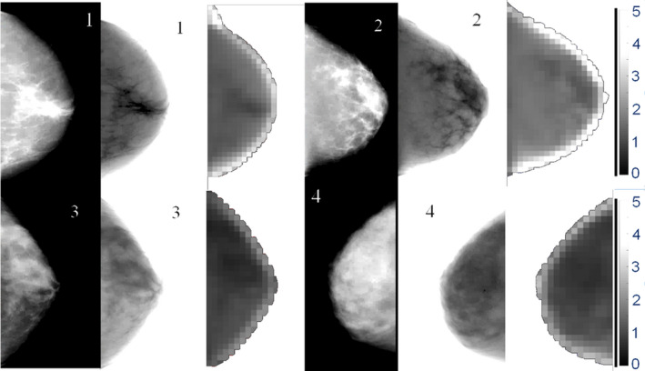
Raw data mammograms (CC View) and the respective generated IQF masking maps for sample images with BI‐RADS density 1 (top‐left), 2 (top‐right), 3 (bottom‐left), and 4 (bottom‐right). Scale of IQF values are shown at right and are consistent across images. IQF values closer to zero are represented as darker pixels, indicate higher levels of masking, and are seen in the higher density images. Raw data mammograms have been contrast‐enhanced to better see dense regions, leading to an artifact being seen at the periphery. Pseudo‐presentation mammograms were developed using previously established methods within the lab¹⁶ [Color figure can be viewed at wileyonlinelibrary.com]

The full list of masking variables used in the conditional logistic regression between interval and screen‐detected cancers and their univariate conditional logistic regression results are shown in Table 3. Many of the masking measures had similar AUC levels and ROC curves, as seen in Fig. 3.

Table 3.

List of all masking measures analyzed and their respective AUC and P‐value for the univariate classification and classification after controlling for BI‐RADS density

Masking measure	AUC for each masking measure	P‐value in regression model	AUC after controlling for BI‐RADS density	P‐Value for inclusion of masking measure
IQF Mean	0.60	6.62E‐07	0.68	1.19E‐03
IQF Median	0.61	3.04E‐06	0.68	02.18E‐03
IQF Sum	0.63	8.58E‐11	0.67	2.52E‐06
IQF Entropy	0.59	6.64E‐06	0.68	8.05E‐04
IQF Kurtosis	0.56	0.015	0.67	0.214
IQF Skewness	0.59	1.78E‐04	0.67	7.55E‐02
IQF 10th Percentile	0.61	1.12E‐06	0.69	1.72E‐03
IQF 25th Percentile	0.61	7.02E‐07	0.68	1.17E‐03
IQF 75th Percentile	0.59	4.37E‐06	0.69	2.91E‐03
IQF 90th Percentile	0.60	1.15E‐07	0.68	4.07E‐04
IQF Percent Area below 1	0.59	5.17E‐06	0.68	6.72E‐04
IQF Percent Area below 2	0.60	9.91E‐07	0.68	2.43E‐03
IQF Percent Area below 3	0.58	4.22E‐05	0.68	5.58E‐03
IQF Percent Area below 4	0.58	3.42E‐04	0.68	1.22E‐02
IQF GLCM contrast	0.54	0.032	0.68	4.43E‐02
IQF GLCM correlation	0.58	1.72E‐04	0.67	9.50E‐04
IQF GLCM energy	0.60	8.11E‐07	0.68	4.58E‐05
IQF GLCM homogeneity	0.57	7.68E‐03	0.67	3.91E‐03

IQF: Image Quality Factor, GLCM: Gray Level Co‐Occurrence Matrix, AUC: Area Under the Curve, BI‐RADS: Breast Imaging‐Reporting and Data System.

P‐value for each masking measure is in a univariate logistic regression model with interval cancer vs screen‐detected cancer as the outcome.

Figure 3.

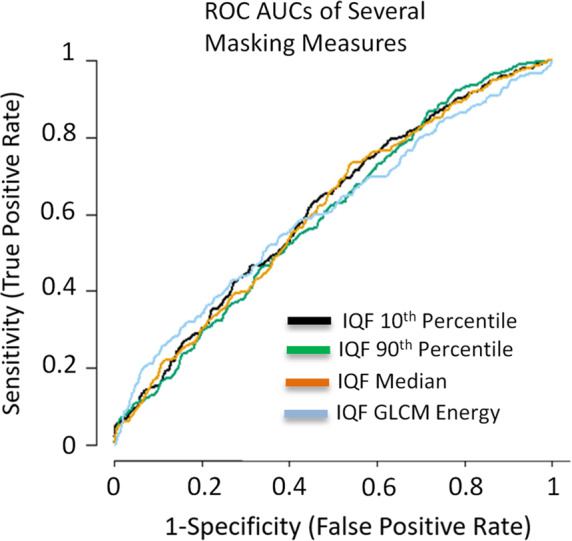
ROC curves for several of the masking measures in predicting interval vs screen‐detected cancer. All masking measures had similar AUCs and ROC curves in the univariate analysis. [Color figure can be viewed at wileyonlinelibrary.com]

Figure 3 shows the ROC curves and associated AUC values of predicting interval and screen‐detected cancer in the test set for the most significant masking measures. These measures improved upon the prediction even after including other breast cancer risk factors.

Figure 4 shows the ROC curves and associated AUC values of predicting interval and screen‐detected cancer of the different models for the IQF 10th percentile, the masking measure that improved the AUC the most compared to the density only model.

Figure 4.

ROC curves of predicting interval vs screen‐detected cancer for the best performing masking measure (IQF 10th percentile). BI‐RADS only ROC curve has circles at each categorical cut point and lines connecting them for clarity. After controlling for BI‐RADS density, this masking measure improves the AUC from 0.65 to 0.69. P‐value for inclusion of masking measure in combined model = 1.7 E‐3. [Color figure can be viewed at wileyonlinelibrary.com]

Several IQF masking measures were statistically significant for inclusion in the conditional logistic regression, even after controlling for BI‐RADS density. Table 4 contains the results of the proportion analysis. In Table 4 we see decreasing proportion of screen‐detected cancers in the groupings with high levels of masking.

Table 4.

Comparison of proportions of screen‐detected cancers by BI‐RADS density groupings and masking measure groupings, grouped by percentiles similar to BI‐RADS density distribution

Masking measure	Measure by quartile
Clinical BI‐RADS density	A	B	C	D	Unknown	Overall
Interval cancers	3	32	77	53	17	182
Screen detected cancers	11	50	61	19	32	173
Proportion of screen‐detected cancers	0.79	0.61	0.44	0.26	0.65	0.49
IQF 10th Percentile	4th	3rd	2nd	1st		Overall
Interval cancers	11	62	84	25		182
Screen detected cancers	25	79	57	12		173
Proportion of screen‐detected cancers	0.69	0.56	0.40	0.32		0.49

IQF: Image Quality Factor, BI‐RADS: Breast Imaging‐Reporting and Data System.

Left most quartiles of the masking measure correspond to the quartile with the lowest masking, and right most quartiles with the highest masking levels.

First to 0–10th percentile of the value of the masking measure.

Second to 10–50th percentile of the value of the masking measure.

Third to 50–90th percentile of the value of the masking measure.

Fourth to 90–100th percentile of the value of the masking measure.

4. Discussion

We identified several measures of masking that are associated with interval compared to screen‐detected cancers even after adjusting for BI‐RADS density. These masking measures may be useful to better identify groups at high risk of interval cancer. The IQF 10th percentile measure provided the largest gain in the AUC when added to the model, raising the AUC from 0.65 with density alone to 0.69. This indicates that these masking measures may contain information about interval breast cancer risk that is not captured in the BI‐RADS density classification alone.

The most significant measure, the 10th percentile of the IQF map, is an indicator of a region of the breast with low detectability. If such a region exists, it follows that a potential cancer would be less likely to be detected by the radiologist in that region of the breast making an interval cancer more likely. The fact that masking measures related to overall, local, and texture qualities indicates that masking properties are complex and need to be further studied to identify all relevant factors at play. Analyzing the proportion of screen‐detected cancers stratified by BI‐RADS density and the IQF 10th percentile measure showed interesting interactions as well. In each case, the proportion of screen‐detected cancers was highest in the low masking category and lowest in the high masking category. The difference between the lowest and the highest proportion was over 30%.

Little has been reported with regards to measuring mammographic masking. Previous work has reported that texture features in presentation mammograms, such as skewness and eccentricity, indicated odds ratios for interval cancer risk of 1.32 and 1.21, respectively. We did not perform a direct comparison to these measures because those measures were performed on presentation mammograms and our analysis only had access to raw data mammograms, but our work was able to further show that there is detectability information in addition to these texture features that are not present in breast density that can aid in interval risk predictions.

Mainprize et al. previously performed a detectability study in which they derive a masking measure by creating a regional detectability index of a Gaussian shaped simulated lesion with a 5 mm FWHM based on the signal to noise ratio, which can be derived from the normalized noise power spectrum, and several other imaging parameters of the mammogram.¹⁰ They found their masking measure correlated with breast density in several different ways and indicated it may be useful to identify risk of interval cancer. Our study expands upon this work by calculating detectability directly with a 2‐AFC test of the model observer and by performing regressions to predict screen‐detected and interval cancers. As the field investigating mammographic masking is growing, future developments, and insights will be gained to best understand how to model and quantify masking.

This study has several strengths. First, it accounts for BI‐RADS density, a known risk factor for interval cancer. This was important because as expected there was a significantly higher proportion of interval cancer cases in the high density categories compared to the screen detected category.^{2, 7} Additionally, matching by age and race between the datasets helps control for confounding in our dataset.

There were several limitations that, if resolved, could improve upon the strength of the study. First, the simulated lesions were rather simplistic in order to optimize insertion and detection testing. There have been several studies showing more advanced models of simulated lesions. Unfortunately, with the current computational ability of our system, implementing these additional calculations for a variety of sizes and thicknesses all throughout the breast was impractical, so we implemented a simpler gaussian model to determine the detectability of a rough lesion simulation. Furthermore, the fact that the 2AFC leveraged a radially averaged power spectrum leaves out certain directionalities in the parenchyma and did not control for the changing thickness and directionality along the skin edge, which could introduce bias in the 2AFC especially along the skin edge.

Another limitation of this work is the small benefit of the additional masking measure over BI‐RADS density, with the improvement mostly being in the lower specificity region. In order to be an effective tool, we would need to have further improvements as well as improvements in the higher specificity range. A more sophisticated model observer such as a Channelized Hotelling filter has the potential to define a stronger interval risk measure.²⁶ However, a NPWE filter may still be sufficient to properly quantify masking and predict risk of interval cancer in mammography, as it performs similarly to detection capabilities in noise similar to breast tissue. Additionally, this study was performed on a case‐case dataset. In the future, comparing masking measures in interval cancers compared to women who do not have breast cancer could help better define the predictive value of the masking measure.

5. Conclusions

In conclusion, the computer vision methods we've developed may be able to identify interval risk information that is not present in BI‐RADS density alone. Further, analysis of proportions of screen‐detected cancers showed that these masking measures provide risk segmentation and may have the potential to identify low density groups at high risk of interval cancer and high density groups with low risk of interval cancer.² This method could be further developed to improve risk prediction models of interval cancer or develop automated methods to help radiologists in risk prediction.

Conflicts of interest

The authors have no relevant conflicts of interest.

Funding

California Breast Cancer Research Program CBCRP #21IB‐0130, National Institutes of Health (NIH, R01CA166945, P01CA154292), National Science Foundation Graduate Research Fellowship Program (NSF, 1144247).

References

- 1. Kerlikowske K. Comparative effectiveness of digital versus film‐screen mammography in community practice in the united states: a cohort study. Ann Intern Med. 2011;155:493. [DOI] [PMC free article] [PubMed] [Google Scholar]
- 2. Kerlikowske K, Zhu W, Tosteson A, et al. Identifying women with dense breasts at high risk for interval cancer: a cohort study. Ann Intern Med. 2015;162:673–681. [DOI] [PMC free article] [PubMed] [Google Scholar]
- 3. Hofvind S, Yankaskas BC, Bulliard J‐L, Klabunde CN, Fracheboud J. Comparing interval breast cancer rates in Norway and North Carolina: results and challenges. J Med Screen. 2009;16:131–139. [DOI] [PubMed] [Google Scholar]
- 4. Holm J, Humphreys K, Li J, et al. Risk factors and tumor characteristics of interval cancers by mammographic density. J Clin Oncol. 2015;33:1030–1037. [DOI] [PubMed] [Google Scholar]
- 5. Gilliland FD, Joste N, Stauber PM, et al. Biologic characteristics of interval and screen‐detected breast cancers. J Natl Cancer Inst. 2000;92:743–749. [DOI] [PubMed] [Google Scholar]
- 6. Sprague BL, Arao RF, Miglioretti DL, et al. National performance benchmarks for modern diagnostic digital mammography: update from the Breast Cancer Surveillance Consortium. Radiology. 2017;283:59–69. [DOI] [PMC free article] [PubMed] [Google Scholar]
- 7. Are You Dense. http://www.areyoudense.org/.
- 8. Malkov S, Shepherd JA, Scott CG, et al. Mammographic texture and risk of breast cancer by tumor type and estrogen receptor status. Breast Cancer Res. 2016;18:122. [DOI] [PMC free article] [PubMed] [Google Scholar]
- 9. Strand F, Humphreys K, Cheddad A, et al. Novel mammographic image features differentiate between interval and screen‐detected breast cancer: a case‐case study. Breast Cancer Res. 2016;18:100. [DOI] [PMC free article] [PubMed] [Google Scholar]
- 10. Mainprize JG, Alonzo‐Proulx O, Jong RA, Yaffe MJ. Quantifying masking in clinical mammograms via local detectability of simulated lesions. Med Phys. 2016;43:1249–1258. [DOI] [PubMed] [Google Scholar]
- 11. ACR . ACR breast imaging reporting and data system atlas. 2013.
- 12. Strand F, Humphreys K, Eriksson M, et al. Longitudinal fluctuation in mammographic percent density differentiates between interval and screen‐detected breast cancer: Strand et al.. Int J Cancer. 2017;140:34–40. [DOI] [PubMed] [Google Scholar]
- 13. Holland K, van Gils CH, Mann RM, Karssemeijer N. Quantification of masking risk in screening mammography with volumetric breast density maps. Breast Cancer Res Treat. 2017;162:541–548. [DOI] [PMC free article] [PubMed] [Google Scholar]
- 14. Mainprize JG, Alonzo‐Proulx O, Alshafeiy T, Patrie JT, Harvey JA, Yaffe MJ. Masking risk predictors in screening mammography. In International Workshop on Breast Imaging, Atlanta GA, 2018. (SPIE) Conference Series; 2018;10718. [Google Scholar]
- 15. Boone JM, Lindfors KK, Cooper VN, Seibert JA. Scatter/primary in mammography: comprehensive results. Med Phys. 2000;27:2408. [DOI] [PubMed] [Google Scholar]
- 16. Malkov S, Wang J, Kerlikowske K, Cummings SR, Shepherd JA. Single x‐ray absorptiometry method for the quantitative mammographic measure of fibroglandular tissue volume. Med Phys. 2009;36:5525. [DOI] [PMC free article] [PubMed] [Google Scholar]
- 17. van Engeland S, Snoeren PR, Huisman H, Boetes C, Karssemeijer N. Volumetric breast density estimation from full‐field digital mammograms. IEEE Trans Med Imaging. 2006;25:273–282. [DOI] [PubMed] [Google Scholar]
- 18. Narod SA. Tumour size predicts long‐term survival among women with lymph node‐positive breast cancer. Curr Oncol 2012;19:249. [DOI] [PMC free article] [PubMed] [Google Scholar]
- 19. Grosjean B, Muller S. Impact of textured background on scoring of simulated CDMAM phantom. In: Digital Mammography. Berlin, Germany: Springer; 2006:460–467. http://link.springer.com/chapter/10.1007/11783237_62. Accessed November 2, 2015. [Google Scholar]
- 20. Samei E, Flynn MJ, Reimann DA. A method for measuring the presampled MTF of digital radiographic systems using an edge test device. Med Phys. 1998;25:102. [DOI] [PubMed] [Google Scholar]
- 21. Eckstein MP, Abbey CK, Whiting JS. Human vs model observers in anatomic backgrounds. In: Medical Imaging'98. Bellingham, WA: International Society for Optics and Photonics; 1998:16–26. http://proceedfings.spiedigitallibrary.org/proceeding.aspx?articleid=943219. Accessed August 31, 2016. [Google Scholar]
- 22. Burgess AE, Jacobson FL, Judy PF. Human observer detection experiments with mammograms and power‐law noise. Med Phys. 2001;28:419–437. [DOI] [PubMed] [Google Scholar]
- 23. Yip M, Chukwu W, Kottis E, et al. Automated scoring method for the CDMAM phantom. In Medical Imaging 2009: Image Perception, Observer Performance, and Technology Assessment. SPIE Conference Series, Lake Buena Vista, FL, 2009;7263:72631A. [Google Scholar]
- 24. Veldkamp WJH, Thijssen MAO, Karssemeijer N. The value of scatter removal by a grid in full field digital mammography. Med Phys. 2003;30:1712. [DOI] [PubMed] [Google Scholar]
- 25. Ciatto S, Bernardi D, Calabrese M, et al. A first evaluation of breast radiological density assessment by QUANTRA software as compared to visual classification. The Breast. 2012;21:503–506. [DOI] [PubMed] [Google Scholar]
- 26. He X, Park S. Model observers in medical imaging research. Theranostics. 2013;3:774–786. [DOI] [PMC free article] [PubMed] [Google Scholar]