Effective nuclei segmentation with sparse shape prior and dynamic occlusion constraint for glioblastoma pathology images

Abstract.

We propose a segmentation method for nuclei in glioblastoma histopathologic images based on a sparse shape prior guided variational level set framework. By spectral clustering and sparse coding, a set of shape priors is exploited to accommodate complicated shape variations. We automate the object contour initialization by a seed detection algorithm and deform contours by minimizing an energy functional that incorporates a shape term in a sparse shape prior representation, an adaptive contour occlusion penalty term, and a boundary term encouraging contours to converge to strong edges. As a result, our approach is able to deal with mutual occlusions and detect contours of multiple intersected nuclei simultaneously. Our method is applied to several whole-slide histopathologic image datasets for nuclei segmentation. The proposed method is compared with other state-of-the-art methods and demonstrates good accuracy for nuclei detection and segmentation, suggesting its promise to support biomedical image-based investigations.

1. Introduction

Image segmentation is a fundamental problem in computer vision and image analysis. In the image segmentation community, level set-based approaches are important tools, because they are able to handle nuclei shapes and contours with complex variations. Chan and Vese initiated a region-based active contour model with a level set formulation based on Mumford-Shah’s functional.^1,2 This model does not depend on gradient information and thus can detect nuclei contours with weak edges. However, Chan–Vese model does not include prior shape knowledge to restrain shapes in appearance and may, therefore, detect meaningless shapes. This drawback becomes more serious when nuclei are partially occluded, corrupted, or represented in low contrast imaging data. In the literature, some research work emerged to mitigate this problem by incorporating shape prior information into the level set formulation so that the detected shape can be regulated by a selected reference shape.^3–5 For example, Chan and Zhu⁶ proposed a variational model introducing a shape difference term with a shape prior as the reference shape.¹ With prior information in place, shapes similar to the shape prior can be successfully segmented. Meanwhile, nuclei presenting meaningless shapes are restrained. Based on the shape prior segmentation model, Yan et al.⁷ introduced a geodesic length term to drive contours to nuclei edges. Ali and Madabhushi⁸ proposed an active contour model to accommodate complex shapes by learning shape priors through principal component analysis.

Nevertheless, shape prior-based level set segmentation methods are still challenged by multiple problems. (1) It is difficult to segment nuclei from raw images without knowing the number and position of nuclei. Thus, one important step in this class of segmentation approaches is to appropriately identify number and positions of nuclei of interest for initialization purpose. (2) Thus far, shape prior-based segmentation approaches exploit libraries consisting of a small number of shape priors as reference to nuclei in similar shapes. However, in most real-world scenarios, such as nuclei segmentation, it could be very complex to model shape variations explicitly. Therefore, it is practically difficult to find a limited number of shape priors that could represent all shapes reasonably well. (3) Simultaneous segmentation of mutually occluded nuclei remains challenging. Recent development in level set methods introduced a repulsion term to prevent two nuclei from becoming identical through evolution. However, it is common to have more than two nuclei involved in mutual occlusion. As a result, we conceive that larger penalties should be given to regions shared by more nuclei.

Nuclei initialization is an important step that guides the following modules in segmentation. The geometric centers of nuclei, so-called seeds, are natural nuclei indicators in practice, as nuclei contours can be appropriately initialized with them. Parvin et al.⁹ proposed an iterative voting method for detecting seeds of overlapping nuclei. Al-Kofahi et al.¹⁰ proposed a multiscale Laplacian of Gaussian (LoG) filtering method for automatic detection and segmentation of nuclei. By distance-map-based adaptive scale selection, nuclear seed points were detected to perform an initial segmentation. However, the multiscale LoG method is sensitive to minor peaks on the distance map, resulting in oversegmentation and detection. Qi et al.¹¹ improved the method by applying a shifted Gaussian kernel and mean shift to a single-pass voting algorithm. The basic idea is to search for the voting direction over a cone-shaped voting area. The two-dimensional (2-D) Gaussian kernel was designed to assign larger weights for area centers in the voting process. Finally, mean shift was applied to determine the seed points.

To accommodate the variation in nuclei shapes, a large set of shape priors can be used as a reference library. However, it is challenging to model the relationship between the nuclei of interest to be segmented and the shape priors. Representation learning methods, such as graph learning and sparse coding, were successfully applied in many areas of computer vision research, such as face recognition,¹² image restoration,¹³ graph learning,¹⁴ and medical image analysis.¹⁵ Wright et al.¹² proposed a robust face recognition algorithm based on sparse representation. The method can effectively handle occlusion and corruption errors by enforcing sparse distribution with respect to the pixel/sample basis. Zhang et al.¹⁵ proposed a sparse shape composition model to incorporate shape prior information for detection and segmentation tasks in radiologic images. Cheng et al.¹⁴ introduced a process to build ${\mathcal{L}}_1$ graph and multiple algorithms for data clustering, subspace learning, and semisupervised learning based on ${\mathcal{L}}_1$ graph. Inspired by theories in graph learning, spectral clustering, and sparse representation, an ${\mathcal{L}}_1$ graph-based shape proximity was learned to cluster the shape priors with which a compact dictionary was created for sparse coding. Given a shape of interest, it can be approximated by a sparse representation based on the compact dictionary within the level set framework. The resulting reconstruction error can be included as a shape penalty term in the variational level set model.

To date, numerous investigators have devised methods to segment overlapping nuclei. These methods extended the shape prior segmentation approaches to segment multiple similar nuclei under mutual occlusion. In Refs. 16–18, various repulsive force terms were proposed and included in the cost functional to penalize two overlapping nuclei contours and prevent them from becoming identical. In our approach, we extend this idea by introducing an adaptive occlusion penalty term that penalizes regions occupied by multiple nuclei based on the scope of occlusion. Following this principle, we assign a larger penalty to a region overlapped by more nuclei.

Recently, deep learning-based approaches greatly improved the state-of-the-art in research fields, such as computer vision, speech recognition, and natural language processing. Deep learning methods require large-scale annotated data to preserve generative power and prevent overfitting. However, collecting both data and annotation for medical imaging tasks is time-consuming and requires much domain expertise. Specifically, a large number of bounding boxes or shape masks of nuclei are required to train the network for deep learning-based nuclei detection and segmentation methods. Compared to the formidable data scale required by deep learning methods, the only prior information used in our method is a set of representative shapes in vector representations with only nuclei contour co-ordinates.

In this paper, we propose a level set-based variational model that allows simultaneous segmentation of multiple nuclei with mutual occlusion. The main contributions of our work are summarized as follows:

• •A seed detection algorithm is proposed to automate nuclei identification and contour initialization. The proposed seed detection algorithm utilizes joint information of spatial connectivity, distance constraint, image edge map, and a shape-based voting map derived from eigenvalue analysis of Hessian matrix across multiple scales.
• •We use a list of contour co-ordinates to represent each annotated nuclei contour. The resulting shape annotation representations are then clustered with an ${\mathcal{L}}_1$ graph-based manifold learning method to establish a concise and representative shape prior library.
• •A sparse representation-based shape term is introduced to better guide nuclei contour convergence with shape prior information from the shape library.
• •A dynamic nuclei occlusion term is proposed to dynamically deal with occlusion events involving a variable number of nuclei.
• •We learn and address the nuclei detection and segmentation problem in an unsupervised manner with no explicit training process in our approach. The only prior information we used is the shape library consisting of shape priors from other glioblastoma histopathology images.
• •Our approach is successfully applied to two datasets of glioblastoma histopathology images for nuclei segmentation task. Our extensive experiments demonstrate that the proposed method can appropriately handle nuclei mutual occlusions and accurately differentiate nuclei from other structures.

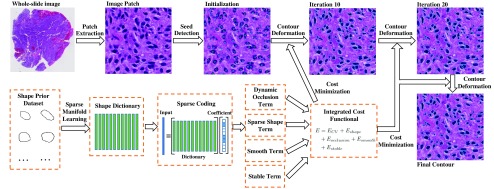
As shown in Fig. 1, our method framework consists of a seed detection algorithm for nuclei contour initialization, and an integrated contour deformable model that incorporates region, shape, and boundary information. The final nuclei contours are converged through an iterative contour evolution process.

Fig. 1.

A schema of our proposed detection and segmentation method for nuclei in histopathologic images.

This journal paper extends our earlier work^19,20 through substantial method improvement on shape prior library generation, more comprehensive experiments, more in-depth parameter sensitivity analysis. In detail, these important extensions include:

• •We include an extensive set of annotated nuclei shapes to include more shape variation information. We propose a way to dynamically construct shape prior dictionary by applying an ${\mathcal{L}}_1$ graph-based manifold learning method. With the approach, representative shape priors covering most shape variations can be automatically produced in a data-driven manner.
• •We provide an in-detail theoretical derivation for level set functional optimization and offer a solution to optimize the loss function.
• •The proposed method is evaluated on two datasets, namely GBM40 dataset and TCGA dataset. The GBM40 dataset consists of glioblastoma tissues from Emory University Hospital archive and TCGA dataset is a publicly available dataset used for method robustness test and efficacy validation. Therefore, we significantly extend our dataset scale for testing and validating the robustness and accuracy of our proposed method in this journal work.
• •We present results from our method for seed detection and nuclei segmentation in different image regions and compare our method with other state-of-the-art methods. In addition, we design multiple analyses with various parameter settings to investigate behaviors of individual terms included in our method. Demonstrated by these extensive tests, the proposed method has manifested promising robustness and accuracy for nuclei detection and segmentation.

2. Shape Representation

Let us consider an image that contains $N$ nuclei of interest ${\mathcal{O}}_1,{\mathcal{O}}_2,\dots ,{\mathcal{O}}_N$, where each nuclei ${\mathcal{O}}_i$ has a closed and bounded shape contour $\partial {\mathcal{O}}_i$ in image domain $\mathrm{\Omega }\subset {\mathbb{R}}^2$. The basic idea of the level set framework is to implicitly represent $\partial {\mathcal{O}}_i$ as a zero level set of a Lipschitz function ${\varphi }_i:\mathrm{\Omega }\to \mathbb{R}$. ${\varphi }_i(\mathbf{x})$ has positive and negative value when $\mathbf{x}$ is inside and outside ${\mathcal{O}}_i$, respectively. Note that due to memory limit, we use image patches instead of whole slide images in our experiments.

2.1. Distance Map Function

A distance map function $\mathrm{\Gamma }[{\varphi }_i(\mathbf{x})]$ represents the shortest distance $d(\mathit{x},\partial {\mathcal{O}}_i)$ from a current pixel $\mathbf{x}$ in the image domain $\mathrm{\Omega }$ to a given nuclei contour $\partial {\mathcal{O}}_i=\{\mathbf{x}|{\varphi }_i(\mathbf{x})=0,\forall \mathbf{x}\in \mathrm{\Omega }\}$:

$$\mathrm{\Gamma }[{\varphi }_i(\mathit{x})]=\{\begin{array}{ll}0,& \mathit{x}\in \partial {\mathcal{O}}_i\\ d(\mathit{x},\partial {\mathcal{O}}_i),& \mathit{x}\in {\mathcal{O}}_i\\ -d(\mathit{x},\partial {\mathcal{O}}_i),& \text{otherwise}\end{array}.$$ (1)

In this way, any nuclei in the image domain can be represented as a distance map or vice versa. Given a distance map, the corresponding nuclei contour can be recovered by searching for the zero-valued pixel locations. As 2-D images only capture 2D projections of 3D nuclei, it is not uncommon to observe overlapped nuclei. Instead of partitioning an image into disjoint regions, we allow a pixel to be associated with multiple nuclei in an image with intersecting contours. Therefore, the corresponding level set functions of all those intersecting nuclei have positive values over the overlapped regions.

2.2. Shape Prior Modelling

Instead of a single shape prior by previous shape prior segmentation methods, we use a large set of shape priors to deal with the complex shape variation observed in most real-world applications. Training shape priors are manually extracted from raw images and aligned with generalized Procrustes analysis,²¹ as illustrated in Fig. 2. The resulting shapes are represented by a set of vectors of uniformly sampled local landmarks: $\{{\gamma }_1,{\gamma }_2,\dots ,{\gamma }_K\}$, where $K$ is the size of the shape prior set.

Fig. 2.

Left: illustration of representative shape priors in the shape prior library. Right: Overlaid 100 shape priors. The shape priors are manually collected by pathologist and serve as shape reference.

For better computational efficiency, the shape priors are partitioned into $M$ clusters, where $M\ll K$. We cluster the shape priors with a learned ${\mathcal{L}}_1$ graph learned by solving the minimization problem for each ${\mathit{\gamma }}_i$:¹⁴

$${\widehat{\mathit{z}}}_i={\Vert {\mathit{\gamma }}_i-B{\mathit{z}}_i\Vert }_2^2+\lambda {\Vert {\mathit{z}}_i\Vert }_1,i=1,\dots ,K\mathrm{s.t.}{z}_{ii}=0,$$ (2)

where $B=({\mathit{\gamma }}_1,{\mathit{\gamma }}_2,\dots ,{\mathit{\gamma }}_K,\mathit{I})$, $\mathit{I}$; is an identity matrix, and $\lambda$ is the parameter balancing the two terms. ${\mathit{z}}_i$ is the $i$’th weighting coefficient and $z_{ij}$ is the $j$’th entry of ${\mathit{z}}_i$. Let $W$ be a graph weight matrix, where each entry $W_{ij}$ represents the similarity between the $i$’th and $j$’th shape priors. We formulate graph matrix as follows:

$$W_{ij}=({\widehat{z}}_{ij}+{\widehat{z}}_{ji})/2,i,j=1,\dots ,K.$$ (3)

With the graph matrix, the un-normalized spectral clustering method^22,23 is used to partition the shape priors into $M$ clusters. The resulting average shape of each cluster is computed and used as a representative shape for the cluster. For simplicity, we denote the corresponding distance maps of the average shapes as $\mathrm{\Psi }=({\psi }_1,{\psi }_2,\dots ,{\psi }_M)$. These distance maps are normalized to have unit Frobenius norm so that the impact of each shape prior is balanced.

2.3. Shape Alignment

To represent a nuclei ${\mathcal{O}}_i$ with shape priors in the training set $\mathrm{\Psi }$, we first align the associated distance map $\mathrm{\Gamma }[{\varphi }_i(\mathit{x})]$ to shape priors by rotation and translation. The transformation from a pixel $\mathit{x}={[x_1{x}_2]}^T$ to the corresponding point ${\tilde{\mathit{x}}}_i$ in shape prior after alignment is formulated as follows:

$${\tilde{\mathit{x}}}_i=s_i\left[\begin{array}{cc}\cos ({\theta }_i)& \sin ({\theta }_i)\\ -\sin ({\theta }_i)& \cos ({\theta }_i)\end{array}\right]\mathit{x}+{\mathit{t}}_i,$$ (4)

where ${\theta }_i$ denotes the rotation angle and ${\mathit{t}}_i={[t_{i1}{t}_{i2}]}^T$ represents the translation displacement. As we observe that all shape priors $\mathrm{\Psi }$ have nearly same scales, we simply set $s_i=1$, $\forall i$ to achieve better computational efficiency.

2.4. Sparse Shape Representation

Given the set of distance maps derived by mapping the $i$’th nuclei to shape prior set $\mathrm{\Psi }({\tilde{\mathit{x}}}_i)$, we assume that the distance map $\mathrm{\Gamma }({\varphi }_i(\mathit{x}))$ of ${\mathcal{O}}_i$ can be approximately represented as a linear composition of shape priors in $\mathrm{\Psi }({\tilde{\mathit{x}}}_i)$. The distance maps and shape priors are vectorized and denoted as $\overline{\mathrm{\Gamma }}[{\varphi }_i(\mathit{x})]$ and $\overline{\mathrm{\Psi }}({\tilde{x}}_i)=({\overline{\psi }}_1,{\overline{\psi }}_2,\dots ,{\overline{\psi }}_M)$, respectively. By the linearity assumption, $\overline{\mathrm{\Gamma }}[{\varphi }_i(\mathit{x})]$ can be represented as follows:

$$\overline{\mathrm{\Gamma }}[{\varphi }_i(x)]=\overline{\mathrm{\Psi }}({\tilde{x}}_i){\alpha }_i+e_i,$$ (5)

where ${\alpha }_i$ is a coefficient vector representing the weights of shape priors in reconstruction and ${\mathit{e}}_i$ is the error vector.

To avoid the curse of dimensionality problem, we reduce $\overline{\mathrm{\Gamma }}$ dimensionality, leading to a less computational cost. The process of dimension reduction can be modeled as left multiplication by a nonzero projection matrix $R\in {\mathbb{R}}^{d\times m}$, $d\ll m$, where $m$ is the total number of pixels in an image. As proved in 12, the choice of matrix $R$ does not critically affect the ability to recover the sparse solution. For computation simplicity, we compose a matrix $R$ with entries randomly generated from standard Gaussian distribution and subject to unit length for all rows. The corresponding low dimension representations are denoted as $\check{\mathrm{\Gamma }}({\varphi }_i)=R\overline{\mathrm{\Gamma }}({\varphi }_i)$, $\check{\mathrm{\Psi }}=R\overline{\mathrm{\Psi }}$, and ${\check{\mathit{e}}}_i=R{\mathit{e}}_i$. Thus, we have

$$\check{\mathrm{\Gamma }}[{\varphi }_i(x)]=\check{\mathrm{\Psi }}({\tilde{x}}_i){\alpha }_i+{\check{e}}_i=\check{\mathrm{\Psi }}({\tilde{x}}_i){\alpha }_i+I{\check{e}}_i,$$ (6)

where $I\in {\mathbb{R}}^{d\times d}$ is an identity matrix and ${\breve{e}}_i$ is the reconstruction error. Note that for an overcomplete system $\breve{\mathrm{\Psi }}\in {\mathbb{R}}^{d\times M}$, the linear system of Eq. (6) may not produce a unique solution. Therefore, more constraints on ${\alpha }_i$ and $e_i$ are needed. Similar to face recognition applications,¹² we observe that given a large enough training set, a test shape should be sufficiently represented using a small number of similar shape priors. In addition, the number of corrupted pixels in the original image and the derived distance map is assumed to be small. This suggests that the coefficient vectors ${\alpha }_i$ and $e_i$ can be sparse as most entries are zero. In this way, most dissimilar prior shapes are suppressed due to large penalty measured by the reconstruction error, which enables us to differentiate ${\mathcal{O}}_i$ from dissimilar shape priors. To ensure the sparsity, we use ${\mathcal{L}}_0$ norm regularization in the formulation. The sparse representation problem is formulated as follows:

$$\begin{gathered} {\widehat{\alpha }}_i,{\widehat{e}}_i=\underset{{\alpha }_i,{\check{e}}_i}{\arg \min }{\Vert \check{\mathrm{\Gamma }}[{\varphi }_i(x)]-\check{\mathrm{\Psi }}({\tilde{x}}_i){\alpha }_i-I{\check{e}}_i\Vert }_2^2 \\ +{\lambda }_1{\Vert {\alpha }_i\Vert }_0+{\lambda }_2{\Vert {\check{e}}_i\Vert }_0. \end{gathered}$$ (7)

However, the problem of finding the sparsest solution in an underdetermined linear system such as Eq. (7) is proved to be nondeterministic polynomial-time hard.²⁴ Due to recent developments in sparse theory, it has been revealed that such a problem can be solved via ${\mathcal{L}}_1$ relaxation:^25–27

$$\begin{gathered} {\widehat{\alpha }}_i,{\widehat{e}}_i=\underset{{\alpha }_i,{\check{e}}_i}{\arg \min }{\Vert \check{\mathrm{\Gamma }}[{\varphi }_i(x)]-\check{\mathrm{\Psi }}({\tilde{x}}_i){\alpha }_i-I{\check{e}}_i\Vert }_2^2 \\ +{\lambda }_1{\Vert {\alpha }_i\Vert }_1+{\lambda }_2{\Vert {\check{e}}_i\Vert }_1. \end{gathered}$$ (8)

The ${\mathcal{L}}_1$ minimization problem can be solved via standard linear programming methods. By this approach, we obtain the sparse coefficients ${\widehat{\alpha }}_i$ and ${\widehat{e}}_i$ and use the coefficients for sparse reconstruction.

3. Seed Detection

In this section, we present an algorithm to recognize nuclei spatial locations by nuclei seed detection. Nuclei seed detection is essential for the follow up nuclei segmentation, as it decides the number and initial contour locations. The proposed seed detection algorithm utilizes joint information of spatial connectivity, distance constraint, image edge map, and a shape-based voting map derived from eigenvalue analysis of Hessian matrix across multiple scales.

3.1. Initialization and Preprocessing

The pathology images of tumor specimens for routine diagnostics usually contain two primary chemical stains: hematoxylin and eosin (H&E). Hematoxylin presents a dark blue or violet color, which positively binds to nuclei. We decompose signal intensity components of H&E stains in original images and use only signals of hematoxylin stain for analysis. Based on Lambert–Beer’s law, the relationship between the intensity of light entering a specimen $L_i$ and that through a specimen $L_o$ can be characterized as $L_o=L_i{e}^{(-Ab)}$, where $A$ and $b$ are the amount of stain and the absorption factor, respectively. By this law, we can compute the stain-specific strength values with a predefined stain decomposition matrix $M$ and the observed optical density (OD): $Y=-\log (L_o/L_i)$.²⁸ The stain composition matrix $M$ consists of three normalized column vectors representing OD values of red, green, and blue channels from hematoxylin, eosin, and null stain. Therefore, stain specific optical signals can be computed by $X=M^{-1}Y$. We retain the first entry of the resulting stain specific signal vector at each pixel and denote the decomposed hematoxylin channel signal as $I_H$.

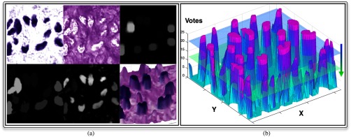
Note that $I_H$ is often coupled with noise produced during the slide preparation process, including uneven tissue slide cut, heterogeneous histology process, staining artifacts, and digital scanning noise. We can normalize the background noise in $I_H$ by morphological reconstruction with two morphological components, namely mask image $I_{\cap }$ and marker image $I_{\cup }$. Initially, we set $I_{\cap }$ as complementary image of $I_H$ and $I_{\cup }$ as $I_H\oplus {\rho }_r$, where $\oplus$ denotes the morphological dilation operator and ${\rho }_r$ is a circular structural element with radius $r$. With marker and mask image, an image $R(I_{\cup },I_{\cap })$ can be reconstructed by iterative dilation and intersection until convergence.²⁹ The difference image $h(I_{\cup },I_{\cap },{\rho }_r)=I_{\cap }-R(I_{\cup },I_{\cap })$ consists of a near zero-level background and a group of enhanced foreground peaks, each representing an object of interest. In Fig. 4(a), we present a typical background normalization result with morphological reconstruction.

Fig. 4.

Voting map derived from a typical image region is demonstrated. (a) Top: the deconvolved hematoxylin channel, eosin channel, marker image; bottom: reconstructed, difference, and voting map surface overlaid with original image. (b) Illustration of the voting peak detection by sliding down an imaginary horizontal plane that intersects with the voting surface.

3.2. Voting Map Construction

Assuming a typical nuclei shape is close to either a circle or an ellipse, we proceed with a shape-based voting process by analyzing nuclei structures within local image regions. Before the voting process, we first enhance nuclei regions by eigenvalue analysis with the Hessian matrix convolved with Gaussian filters at multiple scales.³⁰ With this approach, we search for circular structures based on geometric structures characterized by the neighboring pixel intensity profiles. Specifically, for a pixel at $(i_0,j_0)$, its local image intensity change can be represented by Taylor expansion:

$$\begin{gathered} h_{\sigma }(i_0+\delta i,j_0+\delta j)=h_{\sigma }(i_0,j_0)+(\delta i,\delta j)\mathcal{D}(h_{\sigma }(i_0,j_0)) \\ +\frac{1}{2}(\delta i,\delta j){\mathcal{D}}^2(h_{\sigma }(i_0,j_0)){(\delta i,\delta j)}^T \\ +\mathcal{O}[({\delta }^3)], \end{gathered}$$ (9)

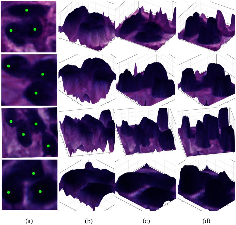
where $h_{\sigma }=h*G_{\sigma }$ and $G_{\sigma }$ is a Gaussian filter with standard deviation $\sigma$; ${\mathcal{D}}^2(h_{\sigma }(i_0,j_0))$ is Hessian of $h_{\sigma }(i_0,j_0)$ that is symmetric and thus diagonalizable with two resulting eigenvalues ${\lambda }_i$, $i=\mathrm{1,2}$, where ${\lambda }_1\le {\lambda }_2$. To make our analysis invariant to nuclei size, we adopt a family of Gaussian filters with distinctive scales to convolve with $h(i,j)$: $G_{{\sigma }_i}$, $i=\mathrm{1,2},\cdots ,S$. As pixels close to nuclei centers have larger intensity values than peripheral points, signs of both eigenvalues for pixels within a nucleus are negative. Even if a nucleus is overlapped with other nuclei, such negative eigenvalue pairs can still be identified at different scales ${\sigma }_i$ within an appropriately chosen scale range because signs of such eigenvalues depend on relative pixel intensity change in nuclei neighborhoods. Leveraging such a signature property of neighboring pixel intensity change, the presence of nuclei, even in clumps, can be indicated by the number of times Hessian matrix produces negative eigenvalue pairs across different Gaussian filter scales. In Fig. 3, we present typical examples of overlapped nuclei with distinct overall clump shapes after different analysis steps. By comparison, voting maps produced from eigenvalue sign analysis encoding pixel intensity profile in nuclei neighborhoods have superior contrast to complementary image of decomposed hematoxylin signal $I_H$ and the difference image $I_h$. It demonstrates that the voting map derived from eigenvalue sign analysis is an effective way to characterize overlapped nuclei local intensity profile features regardless of overall clump shapes. Next, we begin the voting process with a zero-valued voting map for all pixels in the image domain. We only increment the voting map value $V(i,j)$ when ${\lambda }_2(i,j)<0$. If ${\lambda }_2(i,j)>0$, we consider pixel $(i,j)$ is not within a nuclei structure and hence set zero vote for such locations. This process is repeated for all scales. A voting map overlaid with a typical histological image region, where nuclei regions in dark exhibit high votes, is presented in Fig. 4(b).

Fig. 3.

Analysis results of typical examples of overlapped nuclei with distinct overall clump shapes are presented at different steps. (a) Clumped nuclei instances with distinct overall shapes; (b) 3-D illustration of complementary image of decomposed hematoxylin signal surface overlaid with original image; (c) 3-D illustration of the difference image $I_h$ surface after background normalization; and (d) 3-D illustration of voting map after eigenvalue sign analysis.

3.3. Dynamic Seeds Detection and Merging

Given the derived voting map, we dynamically adjust a seed list based on candidate spatial connectivity, distance constraint, and image edge map. The proposed method can produce robust and accurate seed detection result, especially for overlapped nuclei.

As any pixel on the voting map is no larger than the number of scales $S$, we consider the voting map as a surface in a three-dimensional space, as shown in Fig. 4(b). Those strong voting peaks, representing consistent negative eigenvalue pairs from Hessian matrix at different smoothing scales due to radially outward decreasing pixel intensity profiles in local regions, suggest the presence of nuclei. The strong peaks on the voting surface can be detected as we gradually slide down an imaginary horizontal plane (e.g., from the blue to green plane) intersecting with the voting surface. We can generate a binary image from the original voting map with threshold $v$ for each intersection plane. We begin with an empty seed list $L$ and append to it the resulting centroids of voting peaks satisfying all the following conditions: (a) such voting peak centers do not exist in the peak list $L$ yet. (b) They come from strong peaks that suggest consistent local intensity change property, a key to a reliable nuclei detection. Such strong peaks can be identified with their sizes no less than area threshold $A(v)=\eta +\exp [\rho f(v)]$, where $\rho$ and $\eta$ are predefined scalars that determine the lower area threshold for detected peaks in the voting map at each step and $f(v)=\frac{v_{\max }-v}{v_{\max }-v_{\min }}$ is a function normalizing the voting value $v$; specifically, $\eta +1$ is the lowest peak cross-section size expectation when the imaginary horizontal plane is the highest. $\rho$ determines how peak areas are expected to grow as the imaginary horizontal plane slides down. Their choices depend on the nuclei texture homogeneity and nuclei size. We choose $\eta$ to be small enough not to miss any strong peaks, and $\rho$ big enough to represent the rapid growth of strong voting peak cross-sections as the imaginary horizontal plane slides down. (c) Such points are within the foreground region in the binary mask detected by the adaptive thresholding method.

With a list of seed candidates, we perform seed pruning to eliminate false positive seeds. We compute the pairwise distances for all peaks in $L$ and iteratively merge adjacent centroids within distance threshold $D_1$. This is followed by a second round of distance-based merging with a relaxed threshold $D_2$ ($D_1<D_2$). In the second round, two peaks are merged only if the following conditions are true: (a) distance between these two points is less than $D_2$ and (b) the path connecting a pair of points does not intersect with any canny edge derived from the original image. The edge map is used to prevent centroids of closely clumped nuclei from being merged. With this seed merging process, we can retain seeds from true clumped nuclei in histological images without tedious parameter tuning process.

4. Occluded Nuclei Segmentation

With nuclei detected in Sec. 3, we further develop an improved level set based segmentation method to drive initialized nuclei contours to true nuclei edges. Our development is driven by the use case of automatic analysis of occluded nuclei in whole-slide histopathologic images. In our method, each nuclei is described by a level set function and we aim to simultaneously obtain all $N$ level set functions by optimizing a variational model.

4.1. Prior Information Integration

As described in Sec. 2.4, given a large enough set of shape priors $\mathrm{\Psi }=\{{\psi }_j\}$, a shape of interest ${\varphi }_i$ can be encoded as sparse linear superposition of shape priors. Thus, we define a shape term as follows:

$$E_1=\sum _{i=1}^N{\int }_{\mathrm{\Omega }}{[\mathrm{\Gamma }[{\varphi }_i(\mathit{x})]-\sum _{j=1}^M{\psi }_j({\tilde{x}}_i){\widehat{\alpha }}_{ij}]}^2\mathrm{d}x,$$ (10)

where ${\widehat{\alpha }}_{ij}$ is the $j$’th entry of ${\widehat{\alpha }}_i$. This shape prior term describes the difference between the target distance map and the best sparsely reconstructed distance map derived from shape priors. Through this optimization process, the target distance map $\mathrm{\Gamma }({\varphi }_i)$ evolves to fit itself to the feature space spanned by the shape priors.

4.2. Adaptive Penalty on Mutual Occlusion

It is common to have mutually occluded nuclei in 2-D histopathologic images due to the fact that these images represent 2-D projected signals of tissue nuclei in 3-D space. It is a challenging task to segment mutually occluded nuclei and identify hidden boundaries across each other. This problem becomes exponentially complicated when there are more than two nuclei involved in occlusion. In the level set framework, intersecting nuclei may all have positive function values after contour evolutions, making it difficult to differentiate them from each other. To address this problem, we introduce an adaptive occlusion penalty term to dynamically suppress nuclei intersection events. The occlusion penalty term is determined by the number of nuclei that are overlapped. Meanwhile, this term prevents deformable contours from becoming identical after iterations of evolution. Specifically, we define the adaptive occlusion penalty term as follows:

$$E_2={\int }_{\mathrm{\Omega }}\sum _{i=1}^{N}H[{\varphi }_i(x)]-[1-\prod _{k=1}^N(1-H({\varphi }_k(\mathit{x})))]\mathrm{d}x,$$ (11)

where $H(·)$ is the Heaviside function. The first term in Eq. (11) is a superposition of the Heaviside functions of all nuclei at pixel $x$ and the second term is a binary function indicating if pixel $x$ is inside any nuclei. This penalty term describes the extent of image regions occupied by multiple nuclei and the associated number of intersecting nuclei in such regions. Equivalently, it represents a dynamic occlusion penalty power on overlapped nuclei.

4.3. Edge Guided Contour and Evolution Stability

To further encourage contour convergence and retain contour smoothness, we define an edge-guided contour regularity term as follows:

$$E_3=\sum _{i=1}^N{\int }_{\mathrm{\Omega }}Q(x)|\nabla H[{\varphi }_i(x)]|\mathrm{d}x,$$ (12)

where $Q(\mathit{x})=\exp (-\frac{{|\nabla I(\mathit{x})|}^2}{2{\sigma }^2})$ is an exponential function monotonously decreasing as the image magnitude of gradient at $x$ increases and $|\nabla H[{\varphi }_i(x)]|$ is nonzero only on nuclei boundaries. As a result, this term drives contours to strong edge locations and helps to regulate smoothness of nuclei boundaries.

Additionally, we include an evolutionary stability term³¹ to regulate the property of level set function as follows:

$$E_4=\sum _{i=1}^N{\int }_{\mathrm{\Omega }}R(|\nabla {\varphi }_i(x)|)\mathrm{d}x,$$ (13)

where $R(x)$ is defined as a double-well potential function:

$$R(x)=\{\begin{array}{ll}\frac{1}{{(2\pi )}^2}[1-\cos (2\pi x)],& \text{if}x\le 1\\ \frac{1}{2}{(x-1)}^2,& \text{if}x\ge 1\end{array}.$$ (14)

This term in Eq. (13) is used to retain signed distance property for stable level set function computation.

4.4. Improved Variational Level Set Formulation

By combining terms in Eqs. (10)–(13), we formulate our method with a variational level set framework.¹ To evolve nuclei contours to desired nuclei boundaries, we minimize the following functional:

$$\begin{gathered} E(C,\mathrm{\varphi },\mathrm{\Theta },T)={\int }_{\mathrm{\Omega }}\mathcal{L}(x,\mathrm{\varphi },C,\mathrm{\Theta },T)\mathrm{d}x=E_{cv}+\sum _{i=1}^4{E}_i \\ ={\lambda }_o\sum _{i=1}^N{\int }_{\mathrm{\Omega }}{(I-c_i)}^{2}H[{\varphi }_i(x)]\mathrm{d}\mathit{x} \\ +{\lambda }_b{\int }_{\mathrm{\Omega }}{(I-c_b)}^2\prod _{i=1}^N[1-H({\varphi }_i(x))]\mathrm{d}\mathit{x} \\ +\nu \sum _{i=1}^N{\int }_{\mathrm{\Omega }}{[\mathrm{\Gamma }({\varphi }_i(x))-\sum _{j=1}^M{\psi }_j(x_i){\widehat{\alpha }}_{ij}]}^2\mathrm{d}x \\ +\omega {\int }_{\mathrm{\Omega }}\sum _{i=1}^{N}H[{\varphi }_i(x)]-[1-\prod _{k=1}^N(1-H({\varphi }_k(x)))]\mathrm{d}x \\ +\mu \sum _{i=1}^N{\int }_{\mathrm{\Omega }}Q(x)|\nabla H[{\varphi }_i(x)]|\mathrm{d}x+\xi \sum _{i=1}^N{\int }_{\mathrm{\Omega }}R(|\nabla {\varphi }_i(x)|)\mathrm{d}x, \end{gathered}$$ (15)

where $\{c_i\}$ and $c_b$ are scalars that define the average pixel intensities in regions of nuclei and background, respectively. We denote $C=\{c_i,c_b\}$, $\mathrm{\varphi }=\{{\varphi }_i\}$, $\mathrm{\Theta }=\{{\theta }_i\}$, and $T=\{t_{i1},t_{i2}\}$, $i=\mathrm{1,2},\dots ,N$ as sets of variables of the energy functional. Parameters $\{{\lambda }_o,{\lambda }_b,\mu ,\xi ,\omega ,\nu \}$ are weights of different terms in the functional.

5. Numerical Computations

In this section, we present numerical computations to minimize the functional in Eq. (15). We optimize the functional iteratively by updating functions $\mathrm{\varphi }$ and variables $\{C,\mathrm{\Theta },T\}$ alternatively. We begin with updating functions $\mathrm{\varphi }$ first. Parameterizing iteration as an artificial time variable $t>0$, we minimize the functional by solving Euler–Lagrange equation based on theory of calculus of variations:

$$\begin{gathered} \frac{\partial {\varphi }_i}{\partial t}=-\frac{\partial E}{\partial {\varphi }_i}=-(\frac{\partial \mathcal{L}(\mathbf{x},{\varphi }_i)}{\partial {\varphi }_i}-\sum _{j=1}^2\frac{\partial }{\partial x_j}(\frac{\partial \mathcal{L}(\mathbf{x},{\varphi }_i)}{\partial \frac{\partial {\varphi }_i}{\partial x_j}}\left)\right) \\ =-{\lambda }_o{(I-c_i)}^2\delta ({\varphi }_i) \\ +{\lambda }_b{(I-c_b)}^2\prod _{k=1,k=i}^N(1-H({\varphi }_k(\mathit{x})))\delta ({\varphi }_i) \\ +\mu \delta ({\varphi }_i)(\nabla Q(\mathit{x})·\frac{\nabla {\varphi }_i}{|{\varphi }_i|}+Q(\mathit{x})div(\frac{\nabla {\varphi }_i}{|\nabla {\varphi }_i|}\left)\right) \\ +\xi div(\frac{R^{\prime }(|\nabla {\varphi }_i|)}{|\nabla {\varphi }_i|}\nabla {\varphi }_i) \\ -\omega \delta ({\varphi }_i)(1-\prod _{k=1,k=i}^N(1-H({\varphi }_k(\mathit{x})))) \\ -2\nu (\mathrm{\Gamma }({\varphi }_i(\mathit{x}))-\sum _{j=1}^M{\psi }_j({\tilde{\mathit{x}}}_i){\widehat{\alpha }}_{ij}), \end{gathered}$$ (16)

where $\delta (·)=H^{\prime }(·)$ denotes the Dirac delta function.

Next, we fix $\mathrm{\varphi }$ and update transformation parameters. We derive updating equations for transformation parameters by computing gradient descent of functional $E(\mathrm{\Theta },T)$:

$$\begin{gathered} \frac{\partial {\theta }_i}{\partial t}=2\nu {\int }_{\mathrm{\Omega }}(\mathrm{\Gamma }({\varphi }_i(\mathit{x}))-\sum _{j=1}^M{\psi }_j({\tilde{\mathit{x}}}_i){\widehat{\alpha }}_{ij}) \\ (\sum _{j=1}^M({\nabla }_{{\tilde{\mathit{x}}}_i}{\psi }_j·{\nabla }_{{\theta }_i}{\tilde{\mathit{x}}}_i){\widehat{\alpha }}_{ij})\mathrm{d}\mathbf{x}, \end{gathered}$$ (17)

where ${\nabla }_{{\tilde{\mathit{x}}}_i}{\psi }_j\triangleq {\left[\begin{array}{c}\frac{\partial {\psi }_j}{\partial {\tilde{x}}_{i1}}\frac{\partial {\psi }_j}{\partial {\tilde{x}}_{i2}}\end{array}\right]}^T$ and ${\nabla }_{{\theta }_i}{\tilde{\mathit{x}}}_i=\left[\begin{array}{c}{s}_i(-x_1\sin ({\theta }_i)+x_2\cos ({\theta }_i))\\ s_i(-x_1\cos ({\theta }_i)-x_2\sin ({\theta }_i))\end{array}\right]$

$$\begin{gathered} \frac{\partial t_{ik}}{\partial t}=2\nu {\int }_{\mathrm{\Omega }}(\mathrm{\Gamma }({\varphi }_i(x))-\sum _{j=1}^M{\psi }_j({\tilde{x}}_i){\widehat{\alpha }}_{ij}) \\ (\sum _{j=1}^M({\nabla }_{{\tilde{\mathit{x}}}_i}{\psi }_j·{\nabla }_{t_{ik}}{\tilde{x}}_i){\widehat{\alpha }}_{ij})\mathrm{d}x, \end{gathered}$$ (18)

where $k=1$ or 2:

$${\nabla }_{t_{ik}}{\tilde{x}}_i=\{\begin{array}{cc}{[\begin{array}{cc}1& 0\end{array}]}^T,& \text{if}k=1\\ {[\begin{array}{cc}0& 1\end{array}]}^T,& \text{if}k=2\end{array}.$$ (19)

Finally, we fix $\mathrm{\varphi }$, and $\{\mathrm{\Theta },T\}$, and update $c_i$ and $c_b$ by setting the partial derivative of $E(c_i,c_b)$ with respective to $c_i$ and $c_b$ and solving these equations, respectively. The optimal values turn out to be the average image intensities in corresponding area:¹

$$\frac{\partial E(c_i,c_b)}{\partial c_i}=0\Rightarrow c_i=\frac{{\int }_{\mathrm{\Omega }}I(x)H({\varphi }_i)\mathrm{d}x}{{\int }_{\mathrm{\Omega }}H({\varphi }_i)\mathrm{d}x},$$ (20)

$$\frac{\partial E(c_i,c_b)}{\partial c_b}=0\Rightarrow c_b=\frac{{\int }_{\mathrm{\Omega }}I(x)\prod _{i=1}^N[1-H({\varphi }_i(x))]\mathrm{d}x}{{\int }_{\mathrm{\Omega }}\prod _{i=1}^N[1-H({\varphi }_i(x))]\mathrm{d}x}.$$ (21)

In this way, this minimization problem is solved by iterative computation of Euler–Lagrange equation and gradient descent approach until the functional is converged. The zero level sets of the converged functions $\mathrm{\varphi }$ indicate the final nuclei contours.

6. Experimental Results

6.1. Dataset and Parameter Setting

We present experimental results of our algorithm for analysis of nuclei within histopathologic images of glioblastoma brain tumor specimens. The effectiveness of our algorithm is verified with two datasets of H&E stained GBM specimens captured at $40\times$ magnification, namely GBM40 dataset and TCGA FFPE dataset: http://cancergenome.nih.gov/. These images are obtained after glioblastoma brain tissues are processed with a tissue preparation protocol. Image patches with size $512\times 512$ are used for experiments due to memory limit. For GBM40 dataset, there are 5396 and 1849 manually annotated nuclei for seed detection and boundary delineation, respectively. For TCGA dataset, the total number of annotated nuclei for boundary segmentation is 4961. Shape profiles of 27,000 glioblastoma brain nuclei are manually extracted from the dataset to form the set of shape priors. All shape priors are aligned with generalized Procrustes analysis.²¹ As discussed in Secs. 2.1 and 2.2, we represent shapes as distance maps, cluster shape priors with an $L_1$ graph into $M$ groups and use one representative shape from each group to form a training shape dictionary $\mathrm{\Psi }$ for sparse representation. We apply the proposed method to datasets with the following parameter setup: $r=10$, ${\sigma }_i=\{3.3,3.6,\dots ,10\}$, $D_1=15$, $D_2=25$, ${\lambda }_o={\lambda }_b=1$, $\mu =5000$, $\xi =2$, $\omega =2000$, $\nu =3000$, $M=100$, $\eta =10$, $\rho =10$. Note that our approach is an image data driven process. Therefore, the scanner setting such as magnification factor does not have significant impact on the parameter setting. As seeds are detected in the voting map that is produced by eigenvalue analysis of image local Hessian matrix associated with a set of Gaussian filter scales, transforming from the original image to voting map can partially help take care of nuclei scale variations. In our study, this set of Gaussian filter scales is chosen to cover varying nuclei sizes, with $3{\max }_i({\sigma }_i)$ approximately equal to the radius of a typical large nucleus.

For the weighting parameters for nuclei segmentation, we assign parameter values so that all terms in Eq. (15) are appropriately balanced in numerical values. In our experiment, following three parameters have similar value and scale: the coefficient for edge-gradient weighted contour length $\mu$, the coefficient for the occlusion penalty term $\omega$, and the coefficient for squared fitting error of shape-derived distance map $\nu$. The weight $\xi$ is numerically set by referring to typical value of the double-well potential function. We use the l1-ls MATLAB toolbox³² to solve the ${\mathcal{L}}_1$-minimization problem.

6.2. Seed Detection

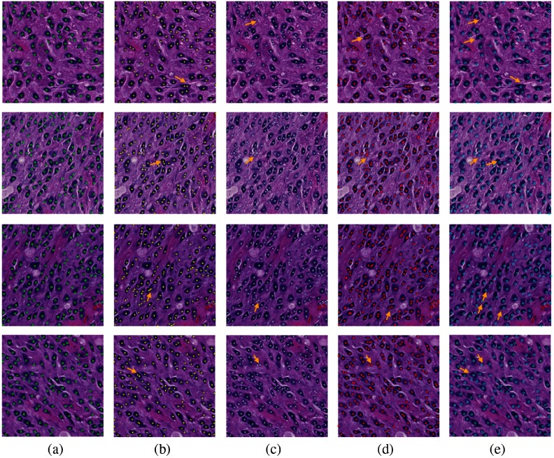
For quantitative analysis, we assess performance of seed detection method with reference to annotations by a pathologist. Note that we evaluate our approach with nontouching and occluded nuclei in each image separately. Five metrics are computed from each image to show seed detection performance: nuclei number error ($C$), miss detection ($M$), false recognition ($F$), over segmentation ($O$), under segmentation ($U$), and count error (CE)%. Nuclei number error is used to demonstrate the absolute difference between the number of nuclei detected by machine and that reported by human expert. Miss and false detection represent the number of missing and false recognition events when machine-based seed detection method is used to detect individual nuclei with no occluded neighbors. Meanwhile, we use over- and undersegmentation to record events where the number of machined-identified nuclei from a nuclei clump is more and less than the true number marked by human expert, respectively. Finally, we use the count error% to represent the nuclei number error in reference to the true nuclei number. The resulting outputs are shown in Tables 1 and 2. Additionally, we compare our method with a single-pass voting method based on mean shift¹¹ and an oriented kernel-based iterative voting method.⁹ By contrast to our method, both the single-pass voting method and the iterative voting method tend to miss detecting nuclei. Note that GBM40 dataset is produced by our local laboratory. Compared to the public TCGA dataset, GBM40 dataset is more carefully prepared with better staining and contrast, leading to higher SNR. This results in better performances of all methods for comparison consistently. We also illustrate seed detection results on several typical image patches in Fig. 5.

Table 1.

Image-wise seed detection performance on GBM40 dataset.

Metric	$C$	$M$	$F$	$O$	$U$	Count error (%)
IVW33	$15.85\pm 8.42$	$2.84\pm 2.23$	$5.76\pm 3.05$	$12.85\pm 5.67$	$0.07\pm 0.27$	11.14
MOW34	$32.15\pm 4.86$	$\mathbf{1.62}\pm \mathbf{1.94}$	$11.15\pm 3.48$	$22.69\pm 4.53$	$0.08\pm 0.28$	22.60
RACM35	$34.46\pm 10.60$	$5.00\pm 2.38$	$7.08\pm 3.88$	$32.08\pm 7.42$	$\mathbf{0.00}\pm \mathbf{0.00}$	24.23
CNN	$32.17\pm 6.61$	$1.67\pm 1.03$	$6.16\pm 2.48$	$27.67\pm 6.15$	$0.00\pm 0.00$	22.65
Ours	$\mathbf{2.15}\pm \mathbf{1.51}$	$2.85\pm 1.99$	$\mathbf{1.30}\pm \mathbf{1.18}$	$\mathbf{0.33}\pm \mathbf{0.66}$	$0.50\pm 0.72$	1.51

Note: Bold numbers indicate the best performance.

Table 2.

Image-wise seed detection performance on TCGA dataset.

Metric	$C$	$M$	$F$	$O$	$U$	Count error (%)
IVW33	$36.85\pm 10.99$	$0.77\pm 0.83$	$32.92\pm 9.28$	$6.31\pm 2.46$	$1.62\pm 1.33$	29.71
MOW34	$55\pm 14.17$	$1.38\pm 1.26$	$55.38\pm 14.55$	$3.62\pm 2.33$	$2.62\pm 1.45$	44.35
RACM35	$54.23\pm 13.28$	$1\pm 1.47$	$42.15\pm 12.42$	$13\pm 5.42$	$0.08\pm 0.28$	43.73
CNN	$48.20\pm 7.59$	$0.00\pm 0.00$	$20.81\pm 9.34$	$27.42\pm 9.81$	$0.00\pm 0.00$	38.87
Ours	$\mathbf{11.92}\pm \mathbf{6.45}$	$2.46\pm 1.20$	$\mathbf{15.69}\pm \mathbf{6.18}$	$\mathbf{1.38}\pm \mathbf{1.56}$	$2.69\pm 1.65$	9.61

Note: Bold numbers indicate the best performance.

Fig. 5.

Comparisons of seed detection results: (a) ground truth; (b) IVW;³³ (c) MOW;³⁴ (d) RACM;³⁵ and (e) our proposed method. We use arrows to demonstrate representative tissue areas, where our approach can correctly detect seeds while other methods fail.

6.3. Nuclei Segmentation

We model the nuclei segmentation problem by the variational level set framework mathematically described in Eq. (15) and solve it by the numerical computations in Sec. 4. The level set functions do not stop evolving until they either reach convergence or exceed iteration number limit. We present the evolution results of zero level sets at iteration 10, 20, and 30 in Fig. 6. The detected nuclei shapes are well defined, as shown in Fig. 6. Notably, those overlapping nuclei can also be correctly segmented, with occluded boundaries reasonably recovered. It is also observed that most zero level sets can rapidly converge to true nuclei boundaries within 10 iterations. After that, zero level sets fine tune themselves to better fit to nuclei contour details, especially over those overlapped nuclei. With our experiment data, we only observe minor improvements in nuclei segmentation from 10 to 30 iterations. In general, the optimal number of iterations depends on data properties. End users can determine the accuracy-speed tradeoff and select the best number of iterations based on individual experiment scenarios.

Fig. 6.

Nuclei contour deformation: initial zero level set and that after 10, 20, 30 evolving iterations, respectively. Those overlapping nuclei can be well separated, as shown in close-up views on the right. (a) The initial contour, (b) 10 iterations, (c) 20 iterations, (d) 30 iterations, and (e) zoomed-in views.

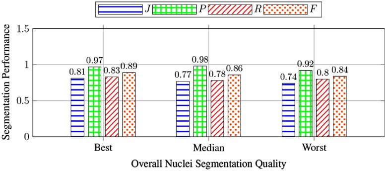
In addition, we present experimental results of three images presenting the best, median, and worst overall segmentation performance in Fig. 7. The bar charts in Fig. 7 present our method efficacy measured by the Jaccard coefficient, precision, recall, and $F_1$ score. The small variation in these metrics over the best, median, and worst images suggests a good consistency and generalization ability of our method.

Fig. 7.

Metrics of the samples with the best, median, and worst Jaccard coefficients overall nuclei segmentation result of all testing images.

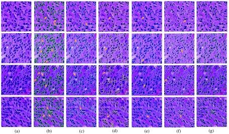
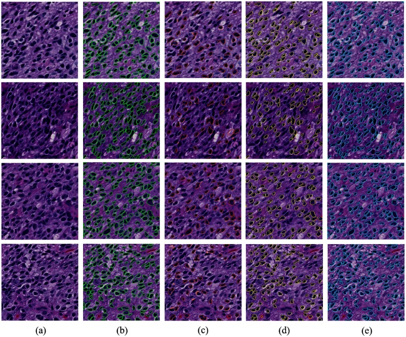
To quantitatively assess our method’s performance, we use human annotations from pathologist as ground truth. By comparing the experimental result $B$ with ground truth annotation $A$, we evaluate the performance of our method with multiple metrics:^36,37 Jaccard coefficient $J(A,B)=\frac{|A\cap B|}{|A\cup B|}$, precision rate $P(A,B)=\frac{|A\cap B|}{B}$, recall rate $R(A,B)=\frac{|A\cap B|}{A}$, F1 score $F_1(A,B)=2\frac{P(A,B)R(A,B)}{P(A,B)+R(A,B)}$, and Hausdorff distance $H(A,B)=\max (h(A,B),h(B,A))$, where $h(A,B)=\underset{a\in A}{\max }\underset{b\in B}{\min }\Vert a-b\Vert$. The testing results evaluated with these metrics are presented in Table 3. Our proposed method achieves better performance in most metrics than the other methods. A qualitative performance comparison across several compared methods and our proposed method is shown in Fig. 8. We also demonstrate the results of the proposed nuclei segmentation method with different seed detection methods in Fig. 10. It is notable that our proposed method is able to better capture nuclei boundaries than other methods for comparison. In particular, only our method can recover boundaries of overlapped nuclei by comparisons. This property makes our method superior to the other methods when analytics of occluded nuclei is crucial in investigations.

Table 3.

The performance comparison of different nuclei segmentation methods measured by region- and distance-based metrics on GBM40 dataset and TCGA dataset.

Methods	GBM40 dataset					TCGA dataset
	$J$	$P$	$R$	$F_1$	$H$	$J$	$P$	$R$	$F_1$	$H$
MS38	$0.44\pm 0.27$	$0.48\pm 0.30$	$0.90\pm 0.17$	$0.56\pm 0.27$	$29.20\pm 28.94$	$0.41\pm 0.26$	$0.52\pm 0.32$	$0.76\pm 0.26$	$0.54\pm 0.27$	$30.12\pm 30.58$
ISO39	$0.59\pm 0.28$	$0.62\pm 0.30$	$0.93\pm 0.15$	$0.69\pm 0.28$	$18.91\pm 29.11$	$0.55\pm 0.26$	$0.61\pm 0.28$	$0.87\pm 0.21$	$0.67\pm 0.25$	$16.34\pm 14.52$
SBGFRLS40	$0.72\pm 0.22$	$0.73\pm 0.22$	$0.98\pm 0.04$	$0.81\pm 0.18$	$9.48\pm 9.66$	$0.68\pm 0.25$	$0.73\pm 0.26$	$\mathbf{0.90}\pm \mathbf{0.15}$	$0.78\pm 0.21$	$14.13\pm 13.02$
IVW33	$0.68\pm 0.18$	$0.74\pm 0.20$	$0.94\pm 0.14$	$0.80\pm 0.15$	$6.53\pm 5.55$	$0.70\pm 0.19$	$0.86\pm 0.16$	$0.82\pm 0.21$	$0.81\pm 0.16$	$6.94\pm \mathbf{6.55}$
MOW34	$0.74\pm 0.20$	$0.79\pm 0.20$	$0.93\pm 0.13$	$0.83\pm 0.16$	$6.22\pm 6.01$	$0.72\pm 0.21$	$\mathbf{0.90}\pm 0.17$	$0.80\pm 0.20$	$0.82\pm 0.17$	$6.90\pm 6.97$
RACM35	$0.63\pm 0.19$	$0.82\pm 0.21$	$0.77\pm 0.19$	$0.75\pm 0.16$	$7.82\pm 6.09$	$0.63\pm \mathbf{0.18}$	$0.89\pm 0.18$	$0.71\pm 0.19$	$0.76\pm 0.16$	$8.08\pm 6.65$
mRLS41	$0.53\pm \mathbf{0}.\mathbf{17}$	$\mathbf{0.83}\pm \mathbf{0}.\mathbf{17}$	$0.64\pm 0.23$	$0.67\pm 0.15$	$10.02\pm 6.65$	$0.51\pm 0.20$	$\mathbf{0.90}\pm \mathbf{0.12}$	$0.56\pm 0.24$	$0.65\pm 0.18$	$10.93\pm 7.33$
CNN42	$0.62\pm 0.25$	$0.74\pm 0.30$	$0.82\pm 0.14$	$0.73\pm 0.22$	$16.41\pm 22.09$	$0.66\pm 0.24$	$0.80\pm 0.26$	$0.83\pm 0.18$	$0.77\pm 0.20$	$11.74\pm 14.51$
Ours	$\mathbf{0.78}\pm \mathbf{0.17}$	$0.79\pm \mathbf{0.17}$	$\mathbf{0.99}\pm \mathbf{0.03}$	$\mathbf{0.87}\pm \mathbf{0.13}$	$\mathbf{4.07}\pm \mathbf{2.76}$	$\mathbf{0.83}\pm 0.24$	$0.89\pm 0.20$	$\mathbf{0.90}\pm 0.20$	$\mathbf{0.88}\pm \mathbf{0.20}$	$\mathbf{4.85}\pm 7.28$

Note: Bold numbers indicate the best performance.

Fig. 8.

Comparison of segmentation results: (a) original image; (b) ground truth; (c) MS;³⁸ (d) ISO;³⁹ (e) SBGFRLS,⁴⁰ (f) vanilla Chan–Vese model,¹ and (g) our proposed method. We use arrows to demonstrate typical tissue areas, where our approach can correctly segment nuclei while other methods fail.

Fig. 10.

Comparison of segmentation results with nuclei initialization by different seed detection methods: (a) original image; (b) ground truth; (c) single-pass voting with mean shift¹¹ using ImageJ plugin; (d) iterative voting;⁹ and (e) our proposed method.

6.4. Parameter Sensitivity Analysis for Segmentation

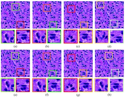
We further investigate the segmentation contribution from individual terms in our variational model by testing with different parameters and comparing their associated segmentation results. The segmentation result with our default parameter setting is shown in Fig. 9(a). When $\nu =0$, the shape prior fitting term $E_1$ does not take effect in the contour deformation process. The resulting segmentation outcome is presented in Fig. 9(b), where finalized nuclei contours are less regulated. Similarly, we can remove the occlusion penalty term $E_2$ from the variational model by setting $\omega =0$. The associated result is illustrated in Fig. 9(c). Under this setting, the detected nuclei present a strong inclination to overlap with each other. When the shape prior fitting term $E_1$, the dynamic occlusion penalty term $E_2$, and the evolutionary stability term $E_4$ are all removed ($\nu =\omega =\xi =0$), the resulting nuclei contours become significantly degraded, as shown in Fig. 9(d). Note that shapes appear to be less regulated in Figs. 9(b)–9(d) without one or more terms in the variational model. In addition to the final results with only a subset of terms in Figs. 9(b)–9(d), we also investigate the sensitivity of parameters to final results. Our investigations with parameter deviation from our proposed value set suggest that results remain similar even when we change $\mu$ by 22% ($\mu =3900$), 10% ($\mu =4500$), and $\nu$ by 67% ($\nu =5000$), as presented in Figs. 9(e)–9(g). Figure 9(h) presents results when $\mu$ and $\nu$ are simultaneously changed by 22% and 67%. Overall, a larger $\mu$ leads to a better contour convergence to true nuclei boundary by energy term $E_3$; a larger $\nu$ forces contours to look more from the reconstructed sparse shape priors by $E_1$; a larger $\omega$ tends to prevent nuclei more from overlapping with each other by $E_2$.

Fig. 9.

Segmented nuclei with distinct parameter settings: (a) $\mu =5000$, $\xi =2$, $\omega =2000$, $\nu =3000$; (b) same as (a) except $\nu =0$; (c) same as (a) except $\omega =0$; (d) same as (a) except $\xi =0$, $\omega =0$, $\nu =0$; (e) same as (a) except $\mu =3900$; (f) same as (a) except $\mu =4500$; (g) same as (a) except $\nu =5000$; and (h) same as (a) except $\mu =3900$ and $\nu =5000$.

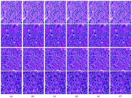
To illustrate the effect of seed detection, we demonstrate the segmented nuclei contours in Fig. 10 by replacing the seed detection algorithm in our pipeline with other seed detection methods. Since the number of detected nuclei depends on the seed-based initialization, miss detection of seeds may result in undersegmentation of nuclei, as shown in Figs. 10(b) and 10(c). We also test the impact of the shape prior library size on segmentation by changing the number of shape prior clusters $M$. The segmented nuclei contours in Fig. 11 show that the proposed method does not degrade significantly with less shape priors. In practice, we carefully choose the number of clusters $M=100$ so that $M$ is large enough to cover shape variations, but small enough to avoid high computation burden.

Fig. 11.

Segmentation with different number of shape clusters: (a) 10; (b) 20; (c) 50; (d) 100; (e) 200; and (f) 300.

6.5. Limitation and Future Work

Although the proposed method can achieve good quantitative and visual results, it is limited by the following factors: (a) Nuclei contour evolution depends on accurate detection of seeds, therefore, the segmentation performance may degrade when seeds are not correctly detected. In cases where seeds are missing, our proposed method, like other level set based methods in literature, does not produce correct segmentation result as no level set function is correctly initialized for deformation. However, we have shown in our experimental tests that our proposed seed detection has a good performance with a very low missing rate, as suggested in Tables 1 and 2. When nuclei seeds are slightly shifted within nuclei regions, our approach is able to produce similar and correct segmented nuclei contours for overlapping nuclei. (b) Application of our method to whole slide images can be time-consuming compared to other state-of-the-art methods. To address the problem, we will further develop a MapReduce based high performance image analysis framework to make this process scalable and cost effective.^43,44

7. Conclusion

In this paper, we propose a nuclei segmentation method based on the level set framework, aiming to simultaneously identify contours of multiple nuclei with mutual occlusion. We present our method with its application to nuclei segmentation using histopathologic images of glioblastoma brain tumors. First, a seed detection method is developed to automatically initialize nuclei contours. For better nuclei contour deformation, we incorporate into the model a set of typical nuclei shapes as prior information through spectral clustering on $L_1$ graph. Meanwhile, an adaptive nuclei occlusion penalty term is designed to dynamically penalize nuclei contour occlusion based on the number of overlapped nuclei. It also prevents recognized contours of overlapped nuclei from being identical. A numerical optimization algorithm is used to iteratively search for the desired level set functions. Experiments on glioblastoma brain histopathologic images produce better results as compared with other state-of-the-art experiments, suggesting the effectiveness of our detection and segmentation approach for nuclei analysis with glioblastoma histopathologic images.

Biographies

Pengyue Zhang is a PhD candidate at the Department of Computer Science at Stony Brook University. His research interests include medical image analysis, computer vision, and machine learning.

Fusheng Wang is an associate professor at the Department of Biomedical Informatics and Department of Computer Science at Stony Brook University. He received his PhD in computer science from the University of California, Los Angeles, in 2004. Prior to joining Stony Brook University, he was an assistant professor at Emory University. His research interest crosscuts data management and biomedical informatics.

George Teodoro received his PhD in computer science from the Universidade Federal de Minas Gerais (UFMG), Brazil, in 2010. Currently, he is an assistant professor in the Computer Science Department at the University of Brasilia (UnB), Brazil. His primary areas of expertise include high performance runtime systems for efficient execution of biomedical and data-mining applications on distributed heterogeneous environments.

Yanhui Liang is works at Google Brain as a software engineer. She received her PhD in biomedical informatics from Stony Brook University. Her research interests include 2-D/3-D medical imaging, computer vision, machine learning, and large-scale spatial data analytics.

Mousumi Roy is a PhD student at Stony Brook University with research focus on computer vision, data analysis, and machine learning modeling for biomedical research.

Daniel Brat received his MD and PhD degrees from Mayo Medical and Graduate Schools. He completed residency and a fellowship at Johns Hopkins Hospital. He is Magerstadt professor and chair of pathology at the Northwestern University Feinberg School of Medicine and pathologist-in-chief of Northwestern Memorial Hospital. He directs a basic and translational research lab that investigates mechanisms of glioma progression, including the contributions of hypoxia, genetics, tumor microenvironment, and stem cells.

Jun Kong received a PhD in electrical and computer engineering from the Ohio State University. Currently, he is an associate professor in the Department of Mathematics and Statistics at Georgia State University. He is an affiliated faculty and a member of the Winship Cancer Institute in Emory university. His primary areas of expertise include biomedical image analysis algorithms, computer-aided diagnosis systems, and large-scale integrative analysis for quantitative biomedical research.

Disclosures

The authors state no conflicts of interest and have nothing to disclose.

References

- 1.Chan T. F., Vese L., “Active contours without edges,” IEEE Trans. Image Process. 10(2), 266–277 (2001). 10.1109/83.902291 [DOI] [PubMed] [Google Scholar]
- 2.Mumford D., Shah J., “Optimal approximations by piecewise smooth functions and associated variational problems,” Commun. Pure Appl. Math. 42(5), 577–685 (1989). 10.1002/cpa.3160420503 [DOI] [Google Scholar]
- 3.Tareef A., et al. , “Automatic segmentation of overlapping cervical smear cells based on local distinctive features and guided shape deformation,” Neurocomputing 221, 94–107 (2017). 10.1016/j.neucom.2016.09.070 [DOI] [Google Scholar]
- 4.Xing F., Xie Y., Yang L., “An automatic learning-based framework for robust nucleus segmentation,” IEEE Trans. Med. Imaging 35(2), 550–566 (2016). 10.1109/TMI.2015.2481436 [DOI] [PubMed] [Google Scholar]
- 5.Lu Z., Carneiro G., Bradley A. P., “An improved joint optimization of multiple level set functions for the segmentation of overlapping cervical cells,” IEEE Trans. Image Process. 24(4), 1261–1272 (2015). 10.1109/TIP.2015.2389619 [DOI] [PubMed] [Google Scholar]
- 6.Chan T., Zhu W., “Level set based shape prior segmentation,” in IEEE Comput. Soc. Conf. Comput. Vision and Pattern Recognit., Vol. 2, pp. 1164–1170 (2005). 10.1109/CVPR.2005.212 [DOI] [Google Scholar]
- 7.Yan P., et al. , “Automatic segmentation of high-throughput RNAi fluorescent cellular images,” IEEE Trans. Inf. Theory. Biomed. 12(1), 109–117 (2008). 10.1109/TITB.2007.898006 [DOI] [PMC free article] [PubMed] [Google Scholar]
- 8.Ali S., Madabhushi A., “An integrated region-, boundary-, shape-based active contour for multiple object overlap resolution in histological imagery,” IEEE Trans. Med. Imaging 31(7), 1448–1460 (2012). 10.1109/TMI.2012.2190089 [DOI] [PubMed] [Google Scholar]
- 9.Parvin B., et al. , “Iterative voting for inference of structural saliency and characterization of subcellular events,” IEEE Trans. Image Process. 16(3), 615–623 (2007). 10.1109/TIP.2007.891154 [DOI] [PubMed] [Google Scholar]
- 10.Al-Kofahi Y., et al. , “Improved automatic detection and segmentation of cell nuclei in histopathology images,” IEEE Trans. Biomed. Eng. 57(4), 841–852 (2010). 10.1109/TBME.2009.2035102 [DOI] [PubMed] [Google Scholar]
- 11.Qi X., et al. , “Robust segmentation of overlapping cells in histopathology specimens using parallel seed detection and repulsive level set,” IEEE Trans. Biomed. Eng. 59(3), 754–765 (2012). 10.1109/TBME.2011.2179298 [DOI] [PMC free article] [PubMed] [Google Scholar]
- 12.Wright J., et al. , “Robust face recognition via sparse representation,” IEEE Trans. Pattern Anal. Mach. Intell. 31(2), 210–227 (2009). 10.1109/TPAMI.2008.79 [DOI] [PubMed] [Google Scholar]
- 13.Mairal J., Elad M., Sapiro G., “Sparse representation for color image restoration,” IEEE Trans. Image Process. 17(1), 53–69 (2008). 10.1109/TIP.2007.911828 [DOI] [PubMed] [Google Scholar]
- 14.Cheng B., et al. , “Learning with -graph for image analysis,” IEEE Trans. Image Process. 19(4), 858–866 (2010). 10.1109/TIP.2009.2038764 [DOI] [PubMed] [Google Scholar]
- 15.Zhang S., et al. , “Sparse shape composition: a new framework for shape prior modeling,” in IEEE Comput. Soc. Conf. Comput. Vision and Pattern Recognit., pp. 1025–1032 (2011). 10.1109/CVPR.2011.5995322 [DOI] [Google Scholar]
- 16.Zhang Q., Pless R., “Segmenting multiple familiar objects under mutual occlusion,” in Proc. Int. Conf. Image Process., 197–200 (2006). 10.1109/ICIP.2006.312454 [DOI] [Google Scholar]
- 17.Le Guyader C., Vese L. A., “Self-repelling snakes for topology-preserving segmentation models,” IEEE Trans. Image Process. 17(5), 767–779 (2008). 10.1109/TIP.2008.919951 [DOI] [PubMed] [Google Scholar]
- 18.Dufour A., et al. , “Segmenting and tracking fluorescent cells in dynamic 3-d microscopy with coupled active surfaces,” IEEE Trans. Image Process. 14(9), 1396–1410 (2005). 10.1109/TIP.2005.852790 [DOI] [PubMed] [Google Scholar]
- 19.Kong J., et al. , “Robust cell segmentation for histological images of glioblastoma,” in Proc. IEEE 13th Int. Symp. Biomed. Imaging, IEEE, pp. 1041–1045 (2016). 10.1109/ISBI.2016.7493444 [DOI] [PMC free article] [PubMed] [Google Scholar]
- 20.Zhang P., et al. , “Automated level set segmentation of histopathologic cells with sparse shape prior support and dynamic occlusion constraint,” in Proc. IEEE 14th Int. Symp. Biomed. Imaging, IEEE, pp. 718–722 (2017). 10.1109/ISBI.2017.7950620 [DOI] [PMC free article] [PubMed] [Google Scholar]
- 21.Goodall C., “Procrustes methods in the statistical analysis of shape,” J. R. Stat. Soc. 53(1), 285–339 (1991). 10.2307/2345744 [DOI] [Google Scholar]
- 22.Mohar B., et al. , “The Laplacian spectrum of graphs,” in Graph Theory, Combinatorics and Applications, Vol. 2, Springer, Berlin, p. 12 (1991). [Google Scholar]
- 23.Mohar B., “Some applications of Laplace eigenvalues of graphs,” Graph Symmetry, Springer, Dordrecht: (1997). [Google Scholar]
- 24.Donoho D. L., Elad M., “Optimally sparse representation in general (nonorthogonal) dictionaries via l1 minimization,” Proc. Natl. Acad. Sci. U. S. A. 100(5), 2197–2202 (2003). 10.1073/pnas.0437847100 [DOI] [PMC free article] [PubMed] [Google Scholar]
- 25.Candes E. J., Romberg J. K., Tao T., “Stable signal recovery from incomplete and inaccurate measurements,” Commun. Pure Appl. Math. 59(8), 1207–1223 (2006). 10.1002/cpa.20124 [DOI] [Google Scholar]
- 26.Candes E. J., Tao T., “Near-optimal signal recovery from random projections: universal encoding strategies?” IEEE Trans. Inf. Theory 52(12), 5406–5425 (2006). 10.1109/TIT.2006.885507 [DOI] [Google Scholar]
- 27.Donoho D. L., “For most large underdetermined systems of linear equations the minimal l1-norm solution is also the sparsest solution,” Commun. Pure Appl. Math. 59(6), 797–829 (2006). 10.1002/cpa.20132 [DOI] [Google Scholar]
- 28.Ruifrok A., Johnston D. A., “Quantification of histochemical staining by color deconvolution,” Anal. Quant. Cytol. Histol. 23(4), 291–299 (2001). [PubMed] [Google Scholar]
- 29.Vincent L., “Morphological grayscale reconstruction in image analysis: applications and efficient algorithms,” IEEE Trans. Image Process. 2(2), 176–201 (1993). 10.1109/83.217222 [DOI] [PubMed] [Google Scholar]
- 30.Frangi A. F., et al. , “Multiscale vessel enhancement filtering,” Lect. Notes Comput. Sci. 1496, 130–137 (1998). 10.1007/BFb0056181 [DOI] [Google Scholar]
- 31.Li C., et al. , “Distance regularized level set evolution and its application to image segmentation,” IEEE Trans. Image Process. 19(12), 3243–3254 (2010). 10.1109/TIP.2010.2069690 [DOI] [PubMed] [Google Scholar]
- 32.Kim S., et al. , “A method for large-scale l1-regularized least squares problems with applications in signal processing and statistics,” IEEE J. Sel. Top. Signal. Process. 1(4), 606–617 (2007). 10.1109/JSTSP.2007.910971 [DOI] [Google Scholar]
- 33.Xu H., Lu C., Mandal M., “An efficient technique for nuclei segmentation based on ellipse descriptor analysis and improved seed detection algorithm,” IEEE J. Bio. Health Info. 18(5), 1729–1741 (2014). 10.1109/JBHI.2013.2297030 [DOI] [PubMed] [Google Scholar]
- 34.Jung C., Kim C., “Segmenting clustered nuclei using h-minima transform-based marker extraction and contour parameterization,” IEEE Trans. Biomed. Eng. 57(10), 2600–2604 (2010). 10.1109/TBME.2010.2060336 [DOI] [PubMed] [Google Scholar]
- 35.Xing F., et al. , “Automatic ki-67 counting using robust cell detection and online dictionary learning,” IEEE Trans. Biomed. Eng. 61(3), 859–870 (2014). 10.1109/TBME.2013.2291703 [DOI] [PubMed] [Google Scholar]
- 36.Fawcett T., “An introduction to roc analysis,” Pattern. Recognit. Lett. 27(8), 861–874 (2006). 10.1016/j.patrec.2005.10.010 [DOI] [Google Scholar]
- 37.Huttenlocher D. P., et al. , “Comparing images using the Hausdorff distance,” IEEE Trans. Pattern Anal. Mach. Intell. 15(9), 850–863 (1993). 10.1109/34.232073 [DOI] [Google Scholar]
- 38.Comaniciu D., Peter M., “Mean shift: a robust approach toward feature space analysis,” IEEE Trans. Pattern Anal. Mach. Intell. 24(5), 603–619 (2002). 10.1109/34.1000236 [DOI] [Google Scholar]
- 39.Grady L., Schwartz E., “Isoperimetric graph partitioning for image segmentation,” IEEE Trans. Pattern Anal. Mach. Intell. 28(3), 469–475 (2006). 10.1109/TPAMI.2006.57 [DOI] [PubMed] [Google Scholar]
- 40.Zhang K., et al. , “Active contours with selective local or global segmentation: a new formulation and level set method,” Image. Vision Comput. 28(4), 668–676 (2010). 10.1016/j.imavis.2009.10.009 [DOI] [Google Scholar]
- 41.Xu H., et al. , “Automatic nuclear segmentation using multi-scale radial line scanning with dynamic programming,” IEEE Trans. Biomed. Eng. PP(99), 1–1 (2017). 10.1109/TBME.2017.2649485 [DOI] [PubMed] [Google Scholar]
- 42.Ronneberger O., Fischer P., Brox T., “U-net: convolutional networks for biomedical image segmentation,” Lect. Notes Comput. Sci. 9351, 234–241 (2015). 10.1007/978-3-319-24574-4 [DOI] [Google Scholar]
- 43.Vo H., et al. , “Cloud-based whole slide image analysis using MapReduce,” in Proc. VLDB Workshop Data Manange. Anal. Med. Healthcare, Springer, pp. 62–77 (2016). 10.1007/978-3-319-57741-8_5 [DOI] [Google Scholar]
- 44.Teodoro G., et al. , “Algorithm sensitivity analysis and parameter tuning for tissue image segmentation pipelines,” Bioinformatics 33(7), 1064–1072 (2017). 10.1093/bioinformatics/btw749 [DOI] [PMC free article] [PubMed] [Google Scholar]