Consideration of sample motion in cryo-tomography based on alignment residual interpolation

Abstract

Recently, it has been shown that the resolution in cryo-tomography could be improved by considering the sample motion in tilt-series alignment and reconstruction, where a set of quadratic polynomials were used to model this motion. One requirement of this polynomial method is the optimization of a large number of parameters, which may limit its practical applicability. In this work, we propose an alternative method for modeling the sample motion. Starting from the standard fiducial-based tilt-series alignment, the method uses the alignment residual as local estimates of the sample motion at the 3D fiducial positions. Then, a scattered data interpolation technique characterized by its smoothness and a closed-form solution is applied to model the sample motion. The motion model is then integrated in the tomographic reconstruction. The new method improves the tomogram quality similar to the polynomial one, with the important advantage that the determination of the motion model is greatly simplified, thereby overcoming one of the major limitations of the polynomial model. Therefore, the new method is expected to make the beam-induced motion correction methodology more accessible to the cryoET community.

Graphical Abstract

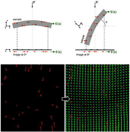
1. Introduction

Beam-induced sample motion is a major resolution limiting factor in cryo-EM (Brilot et al., 2012). The electron irradiation induces the doming of the sample and causes smoothly-varying motion across the illuminated area. This motion blurs the images and degrades its high-resolution components. The direct electron detectors and motion-correction methods have been instrumental for restoring the high-resolution information (Brilot et al., 2012; Zheng et al., 2017). In electron cryo-tomography (cryoET), the standard workflow applies these motion-correction methods to each image of the tilt-series individually (Wan and Briggs, 2016), but the deformation of the sample through the different tilts is often ignored, resulting in tomograms with deteriorated quality (Bharat et al., 2015).

Recently, an alignment approach that takes into account the sample deformation through the tilt-series was introduced in cryoET (Fernandez et al., 2018). It has shown to improve the tilt-series alignment, the tomogram quality and the resolution in subtomogram averaging. The method relies on the fiducial markers embedded in the ice, and uses quadratic polynomial surfaces to model the sample motion in different directions. The model is then applied during reconstruction to yield a motion-compensated tomogram. One requisite for the polynomial sample motion model is the optimization of a large number of parameters, which imposes minimum requirements on the available fiducials for a reliable resulting model. This may limit the practical applicability of the method. To overcome this, here we introduce a novel and alternative strategy to model the sample motion that is based on global splines. The main advantage is its simplicity of determination of the parameters of the model at no performance cost.

2. Background on motion-aware tilt-series alignment

The standard cryoET tilt-series alignment is based on gold particles as fiducial markers. The relationship between the 3D coordinates of the fiducials in the specimen and their coordinates in the images is described by the projection model (Mastronarde, 2006):

$$p_j^i=M^i{r}_j+d^i,i=1\mathrm{...}N,j=1\mathrm{...}{N}_m$$ (1)

where N and N_m are the number of images in the tilt-series and the number of fiducials, respectively, r_j = (x_j, y_j, z_j) are the coordinates of the j-th fiducial marker in the specimen, Mⁱ is the overall projection matrix for the i-th image that encodes the basic parameters (tilt, rotation, magnification) and the projection operator, $p_j^i=\left(u_j^i,v_j^i\right)$ are the coordinates of the projection of the j-th fiducial marker in the i-th image, and dⁱ represents the image shifts with respect to a reference center, typically the centroid of the fiducials.

To consider the sample motion, the projection model in Eq. 1 was extended by introducing a set of quadratic polynomial surfaces that model the 2D motion observed at the projection image level (Fernandez et al., 2018):

$$p_j^i=M^i(r_j)+S^i(r_j)+d^i,i=1\mathrm{...}N,j=1\mathrm{...}{N}_m$$ (2)

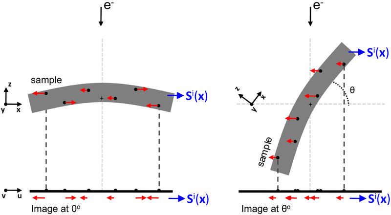
where $S^i(x)=\left(S_u^i(x),S_v^i(x)\right)$, with x = (x, y, z), represents the 2D motion perpendicular to the electron beam direction undergone by the sample in the i-th image, observed at the image plane (u,v) (Fig. 1). These quadratic polynomials $\left(S_u^i(X),S_v^i(x)\right)$ can be either trivariate (i.e. depending on x, y, z; appropriate for thick specimens) or bivariate (i.e. on x, y, thus ignoring the variation along Z and being adequate for thin ones). The formers require 10 parameters whereas the latters need 6 parameters for the expression of the polynomials (Fernandez et al., 2018).

Figure 1. Information about sample motion provided by alignment residuals.

Residuals obtained from the alignment (presented in red color) represent the discrepancy between the experimental and the expected fiducial positions at the image plane (u,v). When the residuals are associated to the 3D coordinates of their fiducials (black dots in the sample), they provide information about the sample motion at scattered positions in the 3D space of the sample (x,y,z). Scattered data interpolation can then be applied to obtain a model of the sample motion Sⁱ(x), as described in the main text. In the figure, the sample coordinate system is represented by (x,y,z). The tilt axis runs along the y axis, perpendicular to the sheet, and is marked by a crosshair in the middle of the sample. The image coordinate system is denoted by (u,v). In this simplified scheme, post-projection rotations are ignored, and v is thus parallel to the tilt axis.

The parameters of the new projection model (Eq. 2) are determined by solving an optimization problem aiming to minimize the sum of squared residuals (discrepancy between the experimental fiducial positions $q_j^i$ and those expected according to the projection model $p_j^i$): $f={\sum }_{i=1}^N{\sum }_{j=1}^{N_m}{\Vert q_j^i-p_j^i\Vert }^2$. This is carried out in two steps (Fernandez et al., 2018). First, a reference tomogram (representing the sample) is set by determining the parameters of the standard projection model (Eq. 1) (i.e. 3D coordinates of the fiducials, r_j, and those associated to the images, Mⁱ, dⁱ). The second step then estimates the polynomial parameters that describe the motion (Sⁱ(x)) undergone by the reference tomogram to account for the experimental fiducial positions deviated from the standard projection model. The total number of required polynomial parameters turn out to be large since there are 2 polynomials per image (2 × N), with 6 or 10 parameters each.

3. Modeling sample motion based on residual interpolation

Instead of the quadratic polynomials previously used, the newly developed method uses global splines to model the sample motion Sⁱ(x). The rationale is that the residuals from the standard alignment (Eq. 1) can provide estimates of the motion (observed at the image plane) with respect to the sample state reflected in the tomogram. Therefore, for each image i in the tilt-series, the residuals

$$q_j^i-p_j^i=q_j^i-(M^i{r}_j+d^i),i=1\mathrm{...}N,j=1\mathrm{...}{N}_m$$ (3)

will provide a discrete set of 2D shifts (perpendicular to the electron beam direction and observed at the image plane) estimated at the scattered fiducial coordinates in the 3D space (r_j) (Fig. 1).

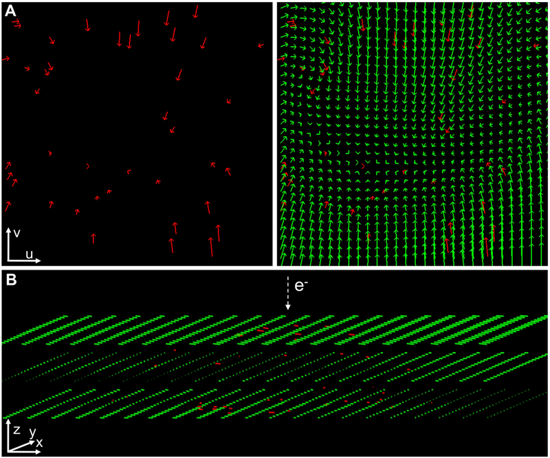
The scattered data interpolation techniques can then be applied to model the sample motion for the entire 3D space, Sⁱ(x), from the sparse and discrete set of residuals $q_j^i-p_j^i$ (Figure 2). We have chosen thin-plate splines (TPS) (Bookstein, 1989), one of the spline interpolation techniques that use radial basis functions (Wolberg, 1990), because of its smoothness (minimal integral of the squared second derivative) and its closed-form solution (coefficients easily determinable by solving a linear equation system). A TPS interpolant is required to model each component of the motion in each image: $S^i(x)=\left(S_u^i(x),S_v^i(x)\right)$.

Figure 2. Estimation of the sample motion at the image plane in 3D by residual interpolation.

(A) An illustrative, simplified 2D case of residual interpolation. Left: residuals at scattered, discrete fiducial positions in a thin sample are presented with red arrows. The initial point of the arrows represents the expected fiducial position according to the standard projection model (i.e. $p_j^i=M^i{r}_j+d^i$) whereas the terminal point represents the experimental position (i.e. $q_j^i$). Right: Sample motion (green vectors) estimated by applying scattered data interpolation over the residuals in (a) (red vectors). For illustrative purposes, the residuals and their interpolated values are shown at the image plane (axes u, v of the image coordinate system; see Fig. 1). (B) Residual interpolation in 3D. Residuals at scattered, discrete 3D fiducial coordinates (r_j) obtained for the untilted image from a thick sample are presented with red lines in the 3D sample coordinate system (axes x,y,z, see Fig. 1). These residuals $\left(q_j^i-p_j^i\right)$ represent shifts perpendicular to the electron beam direction, as observed at the image plane (Fig. 1). After scattered data interpolation, the sample motion is estimated for every point in the tomogram (green vectors; these discrete vectors are represented in a grid and, for clarity, only three Z-planes of this grid are presented). All vectors shown in the figure were scaled 10×.

Interpolation with TPS is accomplished with constraints on the curvature, resulting in the TPS interpolants being as smooth as possible with respect to the second derivatives (Bookstein, 1989). This also ensures a smooth, constrained response in regions far away from the control points (i.e. fiducial coordinates) used in the fitting of the interpolants. In contrast, the polynomials (higher than the first degree) are characterized by an unconstrained behaviour beyond those control points. Thus, TPS interpolation has the potential to produce better models of the sample motion under scarcity of fiducials.

Once the sample motion model is determined for all images by the TPS (i.e. with 2 × N TPS interpolants), the tomogram can be reconstructed with the same strategy as in the polynomial approach (Fernandez et al., 2018). Thus, Weighted Back-Projection (WBP) is applied while the sample motion is compensated for.

In summary, the new method for cryoET tilt-series alignment and reconstruction with consideration of the sample motion consists of four steps:

1. Apply the standard cryoET alignment (Eq. 1) to determine the basic image parameters and, importantly, the 3D coordinates of the fiducials (r_j). This step defines the reference tomogram and the 3D location of the fiducials within it.

2. Compute the residuals $q_j^i-p_j^i$, i.e. the discrepancy between the experimental $(q_j^i)$ and the expected fiducial positions according to the standard projection model $(p_j^i=M^i{r}_j+d^i)$. These residuals are associated to the scattered 3D coordinates of the fiducials (r_j) and define their 2D shifts observed at the image plane due to the doming effect (Fig. 1).

3. Apply TPS interpolation to determine the model that describes the sample motion in the 3D space (Fig. 2B): $S^i(x)=\left(S_u^i(x),S_v^i(x)\right)=\left(\text{TP}{\text{S}}_u^i(x),\text{TP}{\text{S}}_v^i(x)\right)$

4. Reconstruct the tomogram with WBP by including the sample motion model in the projection model: Mⁱ(x) + Sⁱ(x) + dⁱ

3.1. Determination of the TPS interpolants

Each image requires two TPS interpolants to derive the components of the motion $S^i(x)=\left(S_u^i(x),S_v^i(x)\right)=\left(\text{TP}{\text{S}}_u^i(x),\text{TP}{\text{S}}_v^i(x)\right)$ from the N_m fiducials r_j and their residuals $q_j^i-p_j^i$. These TPS interpolants have the form:

$$\text{TPS}(x)\text{\hspace{0.17em}=\hspace{0.17em}}{a}_0+a_{x}x+a_{y}y+a_{z}z+\sum _{j=1}^{N_m}{w}_j\parallel r_j-x\parallel$$ (4)

They are composed of an affine part (with coefficients a), which represents a global transformation, and a non-rigid transformation (the sum term with coefficients w) that is bounded and asymptotically flat (Bookstein, 1989; Wolberg, 1990).

The (N_m + 4) coefficients of each TPS interpolant can be easily determined by solving a linear system of equations established from the interpolation conditions $\left(S^i\left(r_j\right)=q_j^i-p_j^i\right)$ and boundary conditions related to their smoothness (Bookstein, 1989; Wolberg, 1990). Let $\left(\delta u_j^i,\delta v_j^i\right)$ denote the components of the residuals $q_j^i-p_j^i$. Then, the equation system for the u-component of the motion (i.e. $S_u^i(x)$) is:

$$\left[\begin{array}{ll}K\hfill & P\hfill \\ P^T\hfill & O_{4\times 4}\hfill \end{array}\right]\left[\begin{array}{l}{w}_u\hfill \\ a_u\hfill \end{array}\right]=\left[\begin{array}{l}\delta u\hfill \\ O_{4\times 1}\hfill \end{array}\right]$$ (5)

where K is a N_m × N_m matrix with K_ij = ||r_i − r_j||, P is a N_m × 4 matrix whose jth-row is (1, x_j, y_j, z_j), T denotes the matrix transpose operator, O_4×4 and O_4×1 are zero matrices of the indicated dimensions, w_u and a_u are the vectors containing the coefficients of the interpolant $\text{TP}{\text{S}}_u^i(x)$ and δu is the vector with the u-components of the residuals ($\delta u_j^i$, with j = 1 … N_m). A similar system is established for the v-component of the motion, $S_v^i(x)$, from $\delta v_j^i$. The coefficients of the two interpolants $\left({\text{TPS}}_u^i(x),\text{TP}{\text{S}}_v^i(x)\right)$ are then obtained by simply inverting the leftmost matrix in Eq. 5:

$$\left[\begin{array}{cc}{w}_u& w_v\\ a_u& a_{\text{v}}\end{array}\right]={\left[\begin{array}{ll}K\hfill & P\hfill \\ P^T\hfill & O_{4\times 4}\hfill \end{array}\right]}^{-1}\left[\begin{array}{ll}\delta u\hfill & \delta v\hfill \\ O_{4\times 1}\hfill & O_{4\times 1}\hfill \end{array}\right]$$ (6)

The TPS interpolants could be implemented in a bivariate form using the same procedure described above, but removing the coefficient a_z and substituting the 3D Euclidean distance ||·|| in Eqs. 4 and 5 by d² log(d²), with d being the 2D Euclidean distance (Bookstein, 1989; Wolberg, 1990). These bivariate TPS may be useful when the distribution of the fiducials in Z is limited. Here we used trivariate TPS (Eq. 4), unless otherwise stated.

There exists a regularized form of the TPS interpolant (Wolberg, 1990) that replaces the matrix K in Eq. 5 with K + λI, with I being the identity matrix and λ a parameter that allows relaxation of the interpolation condition. Here we used the original formulation (Bookstein, 1989), thereby enforcing exact interpolation (λ = 0), to avoid the need of tuning the parameter.

4. Results

The new method based on residual interpolation with TPS has been tested and compared with the standard alignment and the polynomial motion-compensation method (Fernandez et al., 2018). Two test datasets from samples of different sizes were used: purified T20S proteasomes, ~15 nm in size, which represents a relatively thin sample, and basal bodies (BB), ~300 nm in size, as a representative of a thick sample. The datasets consisted of 14 and 6 tilt-series with a total number of 3928 and 1980 subtomograms (proteasome/BB triplet segments), respectively. Standard alignment and motion estimation was conducted using a range of 26–55 fiducials (for the proteasome) and 22–43 (for the BB). The pixel size was 2.56 and 9.64 Å, respectively. The same datasets were used previously in the polynomial approach work, where the detailed description on the data processing and on the resolution assessment can be found (Fernandez et al., 2018).

4.1. Reduction of alignment residual

Table 1 shows the overall alignment residual, averaged from all tilt-series, from each of the two datasets. For the comparison purpose, the previously reported averaged residual values for the standard alignment and the polynomial motion-compensation method have been included (Fernandez et al., 2018). In the latter case, bivariate and trivariate polynomials were used for the proteasome and BB, respectively, based on their sample thickness. As expected, the mean residual obtained with the new method is 0.0 since it completely compensates for the entire residual found at the fiducial positions.

Table 1.

Alignment residual (pixels)

	Proteasome	Basal Body
	Avg. mean residual
standard alignment	1.83	1.68
polynomial method	0.78	0.99
new TPS method	0.00	0.00
	LOO residual
polynomial method	0.92	1.50
new TPS method	1.03	1.46

An unbiased comparison was carried out based on the Leave-One-Out (LOO) cross-validation test (Kukulski et al., 2011; Fernandez et al., 2018). This is done by leaving one fiducial marker out and modeling the motion (either with polynomials or TPS interpolation) with the remaining fiducials. Based on the resulting motion model, the residual for the excluded fiducial is calculated. The LOO residual for the tilt-series is obtained by repeating this process for all fiducials in the tilt-series and averaging the collected residual values. Table 1 shows the results averaged from all tilt-series in both the proteasome and the BB datasets. They demonstrate that the new TPS method can achieve similar performance compared to the polynomial one, with LOO residual values around 1.0 pixel or 1.50 pixels for the proteasome and BB dataset, respectively. These values are lower than the mean residual from the standard alignment (1.83 and 1.68 pixels, respectively), indicating both approaches produce good models of the sample motion in the entire field of view.

4.2. Improvement in the tomograms and the subtomogram averaging

Tomograms were reconstructed with compensation for the sample motion using the new TPS method. By visual inspection, they looked cleaner and sharper than those from the standard alignment (Suppl. Figure S1). There were subtle, but noticeable, differences in the reconstructed biological features. The improvements in quality with the new TPS method were comparable to those obtained with the polynomial one (Fernandez et al., 2018) (Suppl. Figure S1), further demonstrating that both motion-compensation methods perform similarly well.

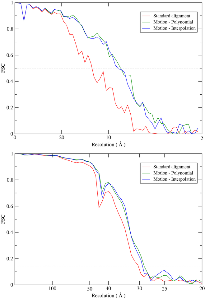
Subtomogram averaging was carried out for the two datasets. Figure 3 shows the FSC curves. The curves for the proteasome were computed against a high-resolution single particle cryoEM map (Grant and Grigorieff, 2015) (EMD-6464) whereas for the BB the Gold-Standard FSC curves from the two data halves are shown. These curves clearly show that the performance of the new TPS method is comparable to the polynomial one. In the proteasome case, the resolution improves from 12.0 (standard alignment) to around 9.0 Å. In the BB case, although the improvement (around 30.5 versus 29.0 Å) is not significant due to other remaining limiting factors (e.g. no. subtomograms, pixel size, CTF, SNR due to thickness), nevertheless, in both cases the FSC curves are above the standard alignment in the entire resolution range.

Figure 3. FSC curves from subtomogram averaging.

Proteasome (top) and Basal Body (bottom). The FSC curves for the proteasome were computed from the subtomogram averages against a high-resolution cryoEM proteasome map. For the BB, the FSC curves were computed from random halves of the data using the gold standard procedure.

4.3. Influence of the abundance of fiducials on the performance

The number of fiducials is known as one of the factors that may affect the accuracy of the motion modeling. Scarcity of fiducials may lead to over-fitting problems, which will translate into mis-modeling of the motion in the areas that are not well covered by the fiducials (Fernandez et al., 2018). To further analyze the performance of the two motion-compensation methods and to check their robustness under these situations, we applied them to the proteasome dataset using different numbers of fiducials for the modeling.

From the full set, we gradually reduced the number of fiducials used in the modeling. Specifically, 12, 9 and 6 fiducials evenly distributed across the field of view were selected. These numbers represent a ratio measurements/unknowns in the optimization of the polynomial parameters of 2.0, 1.5 and 1.0, respectively. In particular, lower ratios might potentially have higher risk of over-fitting problems. Motion modeling was then carried out with both methods using only those subsets of fiducials. Since these small subsets implied a limited Z-distribution of fiducials, both TPS interpolants and polynomials were tested in bivariate form to ensure a fair comparison. The parameters determined by the standard alignment (fiducial coordinates and basic image parameters) using the full set of fiducials were kept here. The performance of the methods was then assessed by cross-validation using the mean residual from the remaining fiducials, which were excluded from the motion modeling (Suppl. Figure S2).

Table 2 shows the averaged results from the 14 tilt-series in the proteasome dataset. With 12 or 9 fiducials being used, the averaged mean residual of the validation fiducials was reduced to around 1 pixel (0.98, 1.02, 1.03, 1.04) regardless of the motion-compensation method. These results are comparable to the LOO residual when the full set of fiducials (in the range 26–55) was employed (Table 1), suggesting that the performance of the methods is not impaired when 12 or 9 fiducials were used in the modeling. However, when motion modeling was done with as few as 6 fiducials, this residual increased and was especially higher in the case of the polynomial method (1.58 versus 1.16 of the new TPS method, see Table 2). These results indicate that the modeling is not so good with such a limited number of fiducials. Analysis of this validation residual for the individual tilt-series (Suppl. Figure S3) showed that the new motion-compensation method is still able to improve it compared to the standard alignment for all tilt-series. In contrast, the polynomial approach failed to improve it for several tilt-series, where over-fitting problems were detected (i.e. increased validation residual compared to the standard alignment and deteriorated quality in certain areas of the tomograms by visual inspection). These results suggest that the new motion-compensation method is more robust than the polynomial one when few fiducials are available.

Table 2.

Cross-validation assessment - averaged mean residual of the validation fiducials (pixels)

	12 fiducials	9 fiducials	6 fiducials
standard alignment	1.85	1.88	1.92
polynomial method	0.98	1.03	1.58
new TPS method	1.02	1.04	1.16

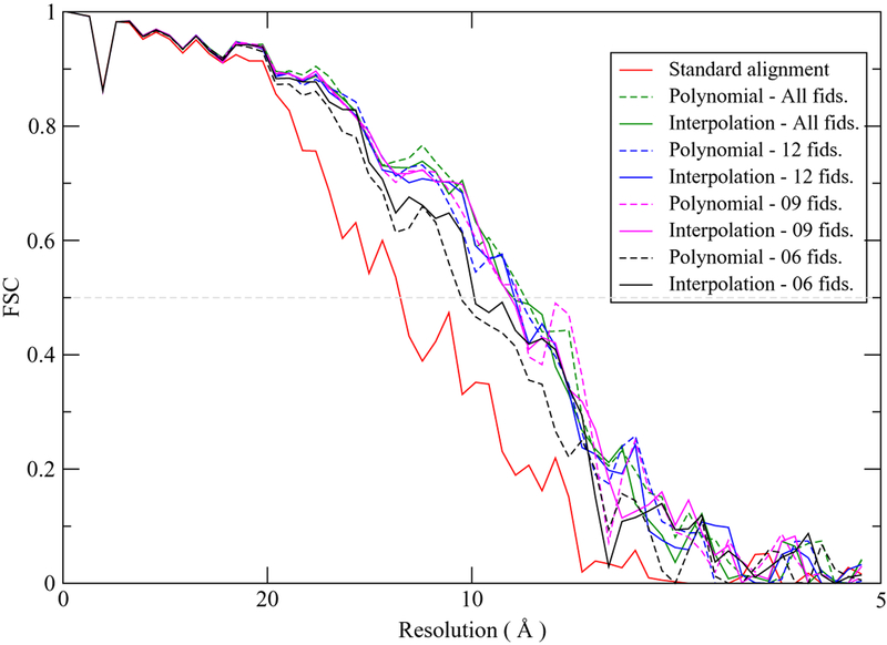
Based on the alignment results, we reconstructed the corresponding tomograms and conducted subtomogram averaging. Figure 4 shows the FSC curves obtained from the resulting averages against a high-resolution proteasome map (EMD-6464). These results are consistent with the validation residuals in Table 2. The FSC curves from both motion-compensation methods are very similar when relatively abundant fiducials (9 or more) are used, with resolutions around 9.0 Å. However, modeling the motion with 6 fiducials resulted in the deteriorated resolutions in both methods, particularly in the polynomial (around 10.5 Å) compared to the new method (around 10.0 Å), as reflected in the FSC curves.

Figure 4.

FSC curves from subtomogram averaging using different number of fiducials for motion modeling.

5. Discussion and conclusion

We have developed a new method to model the sample motion in cryoET. It assumes that the residuals resulting from the standard alignment can be considered as local estimates of the sample motion at the sparse, discrete positions of the fiducials in the 3D space. The sample motion throughout the 3D space can be modeled by using scattered data interpolation techniques. In this work, we have used Thin-Plate Splines (TPS) because of their smoothness and their simplicity of determination of the coefficients, making them very convenient for practical applicability. Indeed, motion modeling can be carried out transparently from the user’s point of view. The model of sample motion can then be directly used in the tomographic reconstruction.

A comparison with the previous polynomial method has shown that the new method produces tomograms of similar quality and similar improvements in resolution in subtomogram averaging. A major advantage of the new method is that their TPS interpolants can be easily constructed by solving a determined linear equation system. This overcomes one of the limitations of the polynomial method: the number of parameters involved and the need for experimental measurements (i.e. fiducial markers) for their reliable fitting. Furthermore, the new method appears to be less susceptible to over-fitting problems when the number of fiducials available is limited. Therefore, the new method may be complementary to the polynomial modeling, in particular when the latter fails or has limited performance. The new method will make this motion-compensation methodology more accessible to the general user in cryoET.

The method presented here partially resembles one of the early developments for motion correction in single particle cryoEM (Nejadasl et al., 2013). There, non-rigid frame alignment (i.e. warping) was carried out from the 2D interpolation of the motion observed at the fiducials in the sample. This 2D warping strategy might also be applied to cryoET of very thin samples, where the motion along the electron path is expected to vary negligibly. Thus, the images could be warped to compensate for the sample motion and produce a pseudo-perfectly aligned tilt-series so that the standard tomographic workflow could be applied. Based on our experience (Suppl. Figure S4), this strategy might be helpful only for very thin samples and the improvement in resolution is still lower than our new method.

The recent evidences indicating that the sample motion is limiting the resolution (Bharat et al., 2015) are driving new developments for tilt-series alignment and reconstruction in cryoET (Fernandez et al., 2018; Himes and Zhang, 2018; Tegunov and Cramer, 2018). These methods apply, adapt or resemble procedures that have been long used to deal with the sample deformation in ET of plastic sections, namely the use of polynomial approximations for optical aberrations and specimen distortions (Lawrence et al., 2006) or the local refinement of the alignment parameters (Mastronarde, 2006; Cantele et al., 2007). These procedures typically require a large number of fiducials, which limits their applicability. Tracking abundant biological structures, or image patches, as virtual fiducials enable reliable local alignment and may provide important improvements in resolution in cryoET (Himes and Zhang, 2018; Tegunov and Cramer, 2018). However, these strategies may be less feasible for relatively thick samples because the amount of overlapping signal may impede successful tracking. Therefore, the new method presented here, based on residual interpolation, will complement the potential role of these emerging techniques in cryoET.

Highlights.

• Alignment residuals provide local estimates of the sample motion at the 3D fiducial positions.

• Scattered data interpolation techniques can be applied to model the sample motion for the entire 3D space.

• The motion model is then integrated in the tomographic reconstruction to yield motion-compensated tomograms.

References

- Bharat TA, Russo CJ, Loewe J, Passmore LA, Scheres SH, 2015. Advances in single-particle electron cryomicroscopy structure determination applied to sub-tomogram averaging. Structure 23, 1743–1753. [DOI] [PMC free article] [PubMed] [Google Scholar]
- Bookstein FL, 1989. Principal warps: thin-plate splines and the decomposition of deformations. IEEE Trans. PAMI 11, 567–585. [Google Scholar]
- Brilot AF, Chen JZ, Cheng A, Pan J, Harrison SC, Potter CS, Carragher B, Henderson R, Grigorieff N, 2012. Beam-induced motion of vitrified specimen on holey carbon film. Journal of Structural Biology 177, 630–637. [DOI] [PMC free article] [PubMed] [Google Scholar]
- Cantele F, Zampighi L, Radermacher M, Zampighi G, Lanzavecchia S, 2007. Local refinement: An attempt to correct for shrinkage and distortion in electron tomography. Journal of Structural Biology 158, 59–70. [DOI] [PMC free article] [PubMed] [Google Scholar]
- Fernandez JJ, Li S, Bharat TAM, Agard DA, 2018. Cryo-tomography tilt-series alignment with consideration of the beam-induced sample motion. Journal of Structural Biology 202, 200–209. [DOI] [PMC free article] [PubMed] [Google Scholar]
- Grant T, Grigorieff N, 2015. Measuring the optimal exposure for single particle cryo-EM using a 2.6 Å reconstruction of rotavirus VP6. Elife 4, e06980, doi: 10.7554/eLife.06980. [DOI] [PMC free article] [PubMed] [Google Scholar]
- Himes B, Zhang P, 2018. High resolution in situ structural determination of heterogeneous specimen. BioRxiv 10.1101/231605. [DOI] [Google Scholar]
- Kukulski W, Schorb M, Welsch S, Picco A, Kaksonen M, Briggs JAG, 2011. Correlated fluorescence and 3D electron microscopy with high sensitivity and spatial precision. Journal of Cell Biology 192, 111–119. [DOI] [PMC free article] [PubMed] [Google Scholar]
- Lawrence A, Bouwer JC, Perkins G, Ellisman MH, 2006. Transform-based backprojection for volume reconstruction of large format electron microscope tilt series. Journal of Structural Biology 154, 144–167. [DOI] [PubMed] [Google Scholar]
- Mastronarde DN, 2006. Fiducial marker and hybrid alignment methods for single and double-axis tomography In: Frank J (Ed.), Electron Tomography. Methods for Three-Dimensional Visualization of Structures in the Cell, 2nd ed. Springer, New York, pp. 163–185. [Google Scholar]
- Nejadasl FK, Karuppasamy M, Newman ER, McGeehan JE, Ravelli RBG, 2013. Non-rigid image registration to reduce beam-induced blurring of cryo-electron microscopy images. Journal of Synchrotron Radiation 20, 58–66. [DOI] [PMC free article] [PubMed] [Google Scholar]
- Tegunov D, Cramer P, 2018. Real-time cryo-EM data pre-processing with Warp. BioRxiv 10.1101/338558. [DOI] [Google Scholar]
- Wan W, Briggs JAG, 2016. Cryo-electron tomography and subtomogram averaging. Methods in Enzymology 579, 329–367. [DOI] [PubMed] [Google Scholar]
- Wolberg G, 1990. Digital Image Warping. IEEE Computer Society Press, Los Alamitos, CA, USA. [Google Scholar]
- Zheng SQ, Palovcak E, Armache JP, Verba KA, Cheng Y, Agard DA, 2017. Motioncor2: Anisotropic correction of beam-induced motion for improved cryo-electron microscopy. Nature Methods 14, 331–332. [DOI] [PMC free article] [PubMed] [Google Scholar]
Associated Data
This section collects any data citations, data availability statements, or supplementary materials included in this article.