Abstract
While many low rank and sparsity based approaches have been developed for accelerated dynamic magnetic resonance imaging (dMRI), they all use low rankness or sparsity in input space, overlooking the intrinsic nonlinear correlation in most dMRI data. In this paper, we propose a kernel-based framework to allow nonlinear manifold models in reconstruction from sub-Nyquist data. Within this framework, many existing algorithms can be extended to kernel framework with nonlinear models. In particular, we have developed a novel algorithm with a kernel-based low-rank (KLR) model generalizing the conventional low rank formulation. The algorithm consists of manifold learning using kernel, low rank enforcement in feature space, and preimaging with data consistency. Extensive simulation and experiment results show that the proposed method surpasses the conventional low-rank-modeled approaches for dMRI.
Index Terms: Low rank models, compressed sensing, kernel method, preimaging, manifold recovery
I. Introduction
DYNAMIC magnetic resonance imaging (dMRI) has been widely used in many clinical applications such as cardiac cine imaging and dynamic contrast enhanced imaging, due to its ability to reveal spatial structures and kinetic information simultaneously. The data acquisition in MRI is modeled mathematically as sampling of the k-space, i.e., the Fourier transform of the desired image. The image is usually reconstructed from these samples using the well-known procedure of truncated Fourier series. In dMRI, to recover the image series using the conventional Fourier reconstruction, the Nyquist sampling criterion has to be satisfied in both k-space and the temporal direction. However, due to the slow data acquisition speed in MRI, this criterion is difficult to satisfy, which results in aliasing artifacts or motion artifacts. Research efforts have been made to reconstruct a high-quality image series from MRI data sampled below the Nyquist rate by exploiting spatial and/or temporal correlations in the image series [1]–[4]. A recent paradigm in sub-Nyquist sampling and signal recovery, Compressed Sensing (CS) has shown promising capability of accelerating data acquisition process without significant loss in signal recovery. Several types of constraints such as sparsity [5]–[17] and low-rankness [3], [18]–[21] have been explored at length in many literature. For example, the partial separable (PS) [18], [19] and sparsity with low rank (SLR) [20] methods suit dynamic data with slow variation, where the temporal basis are approximated nearly accurate from the navigator lines. This assumption is violated when the image series has higher temporal variation such as in perfusion imaging, dynamic imaging with fewer temporal frames and dMRI with motion.
Manifold models [22]–[27] have been widely used in machine learning for nonlinear dimensionality reduction, and it has been shown to be superior to linear approaches such as principal component analysis [28] and multidimensional scaling [29]. However, different from dimensionality reduction applications where the high-dimensional manifold-modeled signal is the input and is not of interest in the output, in image reconstruction, the signal is the output to recover. A few algorithms [30]–[35] have been developed for manifold-modeled signal recovery outside the MRI context. Recently, some papers have studied manifold for dMRI reconstruction [36]–[39]. Specifically, they use the idea of heat kernels and spectral graph theory [25], [40] to characterize the relationship between dMRI image series. For example, in [36], [38], a graph Laplacian is constructed to compute the image similarity, and the eigenfunction of the graph Laplacian provides a smooth embedding for dynamic image series. Such an approach is helpful when the image series consists of highly correlated and distributed image sequence along temporal direction, but might not be effective in the cases when very few temporal frames are available, and/or signal varies significantly along the temporal direction. In the meantime, kernel based methods have also been exploited to learn the intrinsic signal manifold and extensively used for signal embedding, classification, regression and denoising [41]–[43].
In this work, we establish a novel kernel-based framework to learn and incorporate a nonlinear manifold into constrained reconstruction from reduced acquisition. In particular, we use kernel principal component analysis (KPCA) [43], [44] to learn the manifold described by the principal components of the feature space. Low Rank in feature space is enforced by projecting undersampled signal into principal components of features space and preimaging technique is applied to project back the signal from feature space to input image space. We have previously shown that the kernel methods can be used to exploit the nonlinear correlation in the dMRI data [45]–[47]. Here, we put dMRI reconstruction in the context of manifold recovery from compressive measurements which is supported by theoretical results [26], [43], [44]. We use kernel PCA to learn the manifold. Supported by numerical simulations, it is hypothesized that the model learned by kernel PCA can more efficiently (i.e., lower rank in feature space) represent the dynamic images when few temporal frames are acquired, and as a result, the reconstruction based on such a model is more faithful. We thereby propose an efficient manifold recovery algorithm in the kernel-based framework, extending results in our conference papers [46], [47]. Different from kernel compressed sensing [34] which is a nonlinear generalization of sparsity-based reconstruction using kernel dictionary learning, our proposed method is a nonlinear generalization of low rank matrix recovery using kernel principal component analysis. A number of simulation and experimental results are shown to support the hypothesis.
The rest of the paper is organized as follows. In section II-A, we provide a brief review to classical low rank approaches to dMRI. Section II-B presents some background on manifold learning and embeddings and section II-C provides the background of kernel methods, the foundation that our method resides on. Section III elaborates on our proposed method. In section IV, the proposed method is evaluated using extensive simulation and experimental results, followed by discussion on various aspects of the proposed method and results in section V. Finally, section VI concludes the paper.
II. Background Theory
A. Signal recovery under low-rank constraints
In dMRI, the k-space measurement at time t, denoted as d(k, t) can be represented as
| (1) |
where γ (r, t) is the desired dynamic image at time t. The discrete version of dynamic image series can be written as an M ×N Casorati matrix Γ, whose (m, n)th entry is defined as γ(rm, tn), representing the value at the corresponding spatial location and time point [3], [18]. Here, M is the number of voxels in the image and N is the number of frames in the data set. Assuming that data are collected in k-space at a sub-Nyquist sampling rate, the imaging equation can be written as:
| (2) |
where A(·) is a linear operator that performs spatial Fourier transform on the image series with sub-Nyquist sampling and stacks the resulting k-space measurements into a vector y = ℂD, D ≪ MN. Solving Eq. (2) for Γ is a highly ill-posed problem. To address this issue, the low-rank (or partial separability) model has been adopted as the constraint under which the dynamic image series is recovered from under-sampled data [3], [18]–[20]. Specifically, reconstructing γ(r, t) from the undersampled data d(k, t) can be regarded as recovering the low rank Casorati matrix Γ. One way is to use the convex nuclear norm or non-convex Schatten p-norm (p < 1) [20] as surrogates of the rank of Γ. Because the nuclear norm is a convex function, the problem can be solved via semi definite programming:
| (3) |
where ‖·‖* denotes the nuclear norm. An alternative solution is to enforce the low-rank constraint explicitly with a pre-defined rank l by
| (4) |
where Us is a spatial coefficient matrix and Vt a temporal basis. In partial-separability-based methods [3], [18], [19], [48], Vt is usually estimated a priori by applying singular value decomposition (SVD) to the k-space data obtained with temporal Nyquist rate.
B. Manifold
Loosely speaking, a manifold is a topological space which is locally similar to the Euclidean space. The broad class of manifold models arise both in parametric settings where a low-dimensional parameter θ controls the generation of the signal, as well as in non-parametric settings. In parametric settings, for example, manifold models arise when the signals of interest are generated continuously as a function of some d-dimensional parameter. Non-parametric models also arise in many applications where the parameter that controls the generation of manifolds are not known. Both parametric and nonparametric cases are guided by the fundamental assumption that an N dimensional signal xi ∈ ℂN lie on or close to a smooth d dimensional manifold such that d ≪ N, . The goal of manifold learning is to find the low dimensional manifold through some nonlinear dimension reduction methods. Manifold learning has been extensively used in machine learning community for data classification and clustering [49], [50]. However, application of manifold learning in signal recovery is limited due to several challenges such as the lack of sufficient training data, the complexity in learning the manifold model, and the need for preimaging.
C. Kernel Method
Among many manifold learning algorithms, kernel principal component analysis (KPCA) is widely used and has the potential to be applied in signal recovery due to its capability to map testing data onto the embedding obtained from the training data, and the existence of explicit representation of preimages in some cases. Unlike many other approaches such as Isomap [22], Laplacian eigenmaps [25], locally linear embedding [23], and Hessian maps [24] which use local geometry to learn the manifold, KPCA [44] uses global correlation to learn such low-dimensional embedding. KPCA can be considered as a nonlinear generalization of principal component analysis [44].
The idea of kernel method is to nonlinearly transform the data from the original input space to a higher dimensional feature space such that linear operations in the feature space can represent a class of nonlinear operations in the input space. The nonlinear mapping , x → ϕ(x) that maps the input x from establishes a bridge between the input space and feature space . In KPCA, performing the linear PCA operation in the feature space is equivalent to performing a nonlinear PCA in input space, thus achieving the goal of learning the nonlinear manifold.
Specifically, in KPCA [44], the eigenvectors v of the covariance matrix is given by
| (5) |
where is the mean centered data and L is the numbers of signals. These eigenvectors represent the principal components (PC) of the data in the feature space. The coefficients α = [α1, α2, ⋯, αL]T can be found by solving the eigen system equation λv = Σv, or equivalently,
| (6) |
where Kc = K − 1T K − K1T + 1T K1T is the centered kernel matrix,
| (7) |
1L is an L × L matrix with all its elements equals to 1/L, λ and α are the corresponding eigenvalue and eigenvector, and
| (8) |
is the so-called kernel function with denoting inner product in the feature space. Different λ and α contribute to different PCs in the feature space. To map a testing signal x onto the low-dimensional embedding obtained by performing KPCA on the training data, we calculate inner product , where q is the index for the principal components.
It is seen that KPCA does not require explicit calculation of the nonlinear mapping ϕ(x), but only needs knowledge of the kernel functions κ(xi, xj) [44]. The choice of the kernel function (as thus the nonlinear mapping) is critical for the capability of representing the manifold effectively. For example, the Swiss roll manifold cannot be well represented using standard and widely used kernel functions such as Gaussian kernels κ(xi, xj) = exp(−‖xi − xj‖2/c) or polynomial kernels , but can be well represented by constructing data-dependent kernel matrix [42], [44], [51].
In signal recovery, a corrupted testing signal is embedded on the learned low-dimensional manifold. Another fundamental challenge in using the kernel method for signal recovery is that the final embedded testing signal needs to be given in the input space rather than in the feature space. This necessitates the preimaging problem, that finds a so-called preimage such that ϕ(z) = ρ, where ρ is the embedded signal in feature space. Since ϕ is usually highly nonlinear, the preimage does not necessarily exist nor is unique. The choice of kernel leads to different methods of preimaging. For example, for polynomial kernel of the form,
| (9) |
with c ≥ 0 and d being odd, there exists an invertible function fκ such that κ(xi, xj) = fk(〈xi, xj〉). In this case, there exists an explicit expression for the preimage of ϕ(x) and is given by [52, ch.18, pp 544–546]
| (10) |
where ξ is any orthonormal basis of the original input space, and where βq is the projection coefficient of ϕ(x) onto the qth PC vq of the feature space. For many other kernels, preimages can only be obtained through approximations [53], [54].
While KPCA has been widely used in pattern recognition [41], [44], data clustering and classification [49], these applications do not require the preimaging because the desired outputs are only the class that signals belong to, not the recovery of signals in the input space. Some image de-noising applications [34], [55], [56] employ KPCA and preimaging techniques, but require large numbers of training data.
III. Proposed Method
We assume the dynamic image series x lies on a low-dimensional manifold . Let be a nonlinear function that maps the signal x from input space to ϕ(x) in feature space. Using kernel method, we formulate the problem to reconstruct the dynamic image series from undersampled (k, t)-space measurements y as
| (11) |
where are row vectors of Γ representing the temporal profile at each spatial location, is a representation of the row vectors of Γ in the feature space using kernel method, A is combined partial Fourier and vectoring operator that gives a vectored representation y of an undersampled k-space data. The undersampling pattern for y is designed in such way that a few central k-space lines are fully sampled whereas higher frequencies are randomly undersampled at each frame and different random sampling pattens are adopted at different frames, as shown in the Fig. 1. Based on the properties that KPCA is able to reduce the dimension of data nonlinearly, we expect the Casorati matrix to have even lower rank when mapped to the feature space than in the input space with a proper choice of nonlinear mapping function ϕ. Since the manifold on which the dynamic MRI temporal profiles lie is unknown in general, some training data are acquired to learn the underlying manifold. Here we use KPCA to learn the manifold and enforce such manifold structure on the reconstructed image series while ensuring consistency with the k-space measurements. To solve Eq. (11) we use the following three distinct steps: (A) Manifold learning using KPCA, (B) Low rank enforcement in feature Space and (C) Preimaging with data consistency constraint. Step B and Step C are then iterated until convergence. The proposed method can be viewed as a generalization of the PS-based reconstruction method [3] in the feature space, where step (A) is to find the temporal basis in the featu re space using training data, step (B) is to recover the spatial basis and thus the signal in the feature space, and finally step (C) is to map the signal from the feature space to obtain the final image series in the original space.
Fig. 1.

Undersampling pattern used to simulate retrospective undersampling. Left: sampling pattern along phase (Np) - frequency encoding (Nf). Right: phase encoding (Np) - frame (Nfr) direction.
A. Manifold learning using KPCA
The objective of this step is to find the low-dimensional embedding of the dynamic MR images. Since we don’t have knowledge of the desired images, we use the temporal profiles of the low resolution dynamic images as the training data to learn the low-dimensional embedding. Specifically, given a low resolution dynamic image series (Γlow) obtained from zero-filled reconstruction of some central k-space data (typically 15–25 lines), a set of T training signals, pt, t = 1, 2, …, T are formed where each pt is an N dimensional temporal vector from a specific spatial location of the image series. These T (much smaller than the size of the image) training signals are randomly selected from all spatial locations. To learn the low dimensional manifold structure of the dynamic MRI series, we perform KPCA [44], [51] using the training data (xi in Eq. (5) becomes pt). The key idea here is that we represent each principal component in feature space as a weighted combination of nonlinear functions (mappings in feature space) of the training signals, that is
| (12) |
Similar to the PS-based methods where the temporal basis are estimated initially, these principal components in feature space are equivalent to nonlinear temporal basis. If the desired dynamic image series has a low rank representation in feature space, then it can be represented efficiently by very few temporal basis.
B. Low Rank Enforcement in Feature Space
In this step, our objective is to recover the desired dynamic images in feature space. We start with the aliased dynamic images obtained by zero-filled reconstruction of all undersampled k-space data. Under the assumption that the true dynamic images should lie on the low-dimensional manifold learned from step A, we project the aliased dynamic images onto such a low-dimensional manifold. This is realized by enforcing the low rankness on the matrix formed by the aliased dynamic images in the feature space. Specifically, we construct test signals using the temporal profiles of the aliasing dynamic images. Each of the test signals xi, i = 1, 2, …, M represent the corrupted version of the temporal signals of the desired dynamic images such that xi = Γ(i,:). We then project the test signals xi onto the nonlinear temporal basis computed in step A, which is equivalent to mapping the test signals onto the learned low-dimensional manifold. Let vq represent the qth PC in the feature space, the projection of the test signal xi on the qth PC is obtained by
| (13) |
where is the mean centered version of kxp(i) and measures the similarity between the test signal xi and all training signals pt such that,
| (14) |
| (15) |
It is seen from Eq. (13) that KPCA does not require explicit calculation of the nonlinear mapping ϕ(x), to compute the projection coefficients but only requires the knowledge of the kernel functions κ(xi, xj) and α which can be calculated using the eigen decomposition of kernel matrix as shown in Eq. (6). Similar to the PS-based reconstruction methods where a pre-determined number of temporal basis is chosen, we choose Q major principal components (Q ≪ T ≪ M) in the feature space corresponding to the Q largest eigenvalues as the nonlinear temporal basis to efficiently represent the temporal variations at all spatial locations. Hence, is approximated as:
| (16) |
where , and Eq. 16 takes the form of . Then the feature space representation of the test signal takes the form of
| (17) |
where
| (18) |
The expression of the test signal in Eqs. 16 and (17) can be considered as the low rank representation of the dynamic image series in the feature space by truncating the numbers of principal components in feature space and further soft thresholding on as
| (19) |
The soft threshold value is then updated for the next iteration as Sth = Sth −(1−(it − 1)Csstep) where it is the number of iterations and sstep is the step size typically of order 10−5 [21], [57]. It should be noted that, although thresholding is typically not required in dimensionality reduction and classification problems because of the high quality test signals, in our case thresholding is desired because the test signals are corrupted temporal signals obtained from aliased image [21], [57]. Furthermore, our empirical results show that soft thresholding is slightly better than hard thresholding.
C. Preimaging with Data Consistency Constraint
After we calculate all the coefficients , we have obtained , the desired image series in feature space. Different from the conventional PS-based method where the reconstruction is completed after Step B, our proposed method further needs to map the estimated image series from the feature space back into the original input space. Such a mapping is obtained through the so-called preimaging, which relies on the specific kernel function. Here we use the polynomial kernel of κ(xi, xj) = (〈xi, xj〉 + c)d such that the preimage zi of the temporal profile (test signal xi) at the ith spatial location can be obtained by generalization of Eq. (10) as,
| (20) |
After computing preimages for all spatial locations, we have the image series Γ, whose rows are the , i = 1, ⋯, M. To ensure the reconstructed Γ is consistent with the measured undersampled data, the spatial Fourier transform of the dynamic images are replaced by the acquired k-space data at the specific sampled locations while keeping the values at unacquired locations unchanged. Specifically,
| (21) |
where, Γk is the k-space equivalent of Γ, S′ is the binary inversion of the sampling mask S, , is the Casorati form of acquired k-space data (y), and (.*) represents element wise multiplication. Then the updated dynamic image series is obtained by inverse Fourier transform of the updated k-space data Γk. Such an updating process has been widely used in MR image reconstruction [15], [16].
Algorithm 1.
Kernel Low Rank (KLR) Model
| Input: Casorati matrix (Γaq) for image series from undersampled data. |
| Casorati matrix (Γlow) from low resolution training image series. |
| Output: Dynamic Image series (Γ). |
| A. Manifold Learning Using Kernel |
| Construct: pt = Γlow(t,:), t = 1, 2, …, M. |
| Select T random training signals pt. |
| Compute kernel matrix Kp and mean centered , using Eq. (7). |
| Eigen decomposition: . |
| Γ = Γaq. |
| B. Low Rank Enforcement in Feature Space |
| Construct test signals xi = Γ(i,:), i = 1, 2, …, M. |
| for i = 1 : M do |
| for q = 1 : Q do |
| Compute: Kernel vector , using Eq. (15). |
| Compute: Projection coefficients , using Eq. (13). |
| Soft threshold , using Eq. (19). |
| Compute: , using Eq. (18). |
| end for |
| end for |
| Update soft threshold Sth. |
| C. Preimaging with Data Consistency |
| for i = 1 : M do |
| Compute preimage zi, using Eq. (20). |
| Update Γ using . |
| end for |
| Update k-space data, using Eq. (21). |
| if Convergence then |
| Output dynamic image series Γ. |
| else |
| Repeat steps B and C. |
| end if |
The low rank enforcement (III-B) and the data consistency constraint (III-C) steps are then iterated until convergence. The iteration is continued until certain error tolerance criterion is met, such as where ‖·‖F is the Frobenius norm. Typically, etol is set to be in the order of 10−4. Although convergence has not been proved theoretically due to many iterative variables, numerical results show that the proposed method converges empirically. The proposed method is summarized in the Algorithm 1.
IV. Results
We performed simulation and experiments to evaluate the proposed method. Because the temporal variations can be quite different from application to application, our focus was on dynamic perfusion imaging with fewer temporal frames. The pros and cons of the proposed method are also discussed for cardiac cine imaging when the number of temporal frames are higher.
We start with two simulations to validate the proposed model and framework independent of the reconstruction algorithm. The first one is to show kernel PCA can represent the dynamic perfusion phantom images more efficiently than linear PCA, and the second one is to show the training data from low resolution images and from full resolution images generate similar training results. We then use a dynamic perfusion phantom [58] and two sets of in vivo arterial spin labeled (ASL) [59], [60] perfusion dMRI data from calf muscle and myocardium. In all in vivo experiments, the fully sampled data in Cartesian (k, t) space was acquired from an MRI scanner and its conventional Fourier reconstruction was used as the “true” reference for comparison of the reconstruction results from different methods. Besides the proposed method, methods exploiting low rankness in the original spatial-temporal space were also used for reconstruction, including PS with sparsity constraint [18], SLR [20], and CS-PCA [6]. All methods reconstruct the desired dynamic MR images from the retrospectively undersampled (k, t) space data obtained by using the undersampling pattern as shown in the Fig. 1. For the proposed method, all adjustable parameters including the number of principal components and the soft threshold value in feature space were all tuned heuristically. For all other methods, the results were obtained using the code from the corresponding research groups that developed the methods but were modified with the parameters tuned for the least root normalized mean square error (RNMSE) defined in Eq. (22),
| (22) |
where ΓREF and ΓREC are the matrix formed by the dynamic images from the reference and the reconstruction, respectively, and ‖·‖F denotes the Frobenius norm.
All computations were carried out on a DELL workstation with Intel(R) i7 3.40 GHz processor and 16 GB RAM, running MATLAB 2014.
A. Validation using simulations
We first use two simulations to validate the assumptions made in the proposed framework.
Simulation 1
The objective of this simulation is to demonstrate that kernel PCA is more efficient than linear PCA in representing the dynamic MR image series. We used a numeric perfusion phantom of size 256 × 256 with 50 time frames. The perfusion phantom represents liver, portal vein, inferior vena cava and pancreas based on enhancement kinetic modeling [58]. The injection rate, frequency and base vibration amplitude of 4 ml/sec, 500 and 30 respectively were chosen to mimic fast and abrupt temporal variation. From the original image series, 1000 training signals (temporal signals at 1000 spatial locations) were randomly selected and used to compute both linear PCs and kernel PCs. The 256 × 256 test signals (temporal signals at all spatial locations) were then projected onto 5% of the PCs in both linear and KPCA to generate approximations of the dynamic images. For KPCA, polynomial kernel was used and preimaging was performed to obtain the dynamic images for comparison. Figure 2 shows the comparison of spatial results and temporal curves of two regions of interest (ROI). It shows that with the same percentage of PCs, the RNMSE is much lower in KPCA than in linear PCA. The superiority of KPCA is also illustrated by the temporal curves of two ROIs, which suggests that KPCA represents the dynamic images more efficiently than PCA.
Fig. 2.

(i) Comparison of images and (ii) temporal curves of ROIs using linear and kernel PCA. (a) Reference. (b) Approximations using 5% PCs. Top: Linear PCA; Bottom: KPCA. (c) Corresponding error maps magnified ×20. RNMSE: PCA 0.0182 and KPCA 2.9×10⁻⁸, respectively.
Simulation 2
The objective of this simulation is to demonstrate that the training data from low-resolution images is sufficient to learn the low-dimensional embedding of the true, full-resolution images. We replace the training data in Simulation 1 from the true images to the low-resolution images, and perform KPCA approximation again. In Fig. 3, we compare the approximations obtained by low-resolution and full-resolution training data. Both approximations are seen to be very close in the spatial images and temporal variation as shown in Fig. 3. It is evident that the low-resolution images provide sufficient information for training.
Fig. 3.

(i) Comparison of images and (ii) temporal curves of ROIs approximated using training signals from full resolution and low resolution images. (a) Reference. (b) Approximations using 5% of PCs. Top: using training signals from full resolution images; Bottom: using training signals from low resolution images. (c) Corresponding error maps magnified ×107. RNMSE: Full resolution 1.12×10⁻⁸, Low resolution 3.14×10⁻⁷.
B. Phantom Results
A dynamic perfusion phantom with aperiodic motion with 50 temporal frames (refer to section IV-A for data parameters) was used to simulate the reduced (k, t) data with a reduction factor (R) of 5. The spatial results, as shown in the Fig. 4 illustrate that the aliasing artifacts in the conventional state of art methods are significantly reduced by the proposed method. Figure 5 compares the temporal variation of the cross section along the yellow line indicated in the reference image. The improved performance of the proposed method can be attributed to the ability to reveal the low rankness of the dynamic data in a much higher dimensional feature space, whereas the rank in the original space is not as low when there are only a few temporal frames.
Fig. 4.
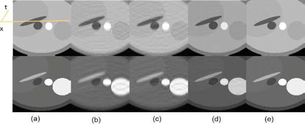
Spatial results: reconstruction comparison for dynamic perfusion phantom with motion. Two representative frames (a) Reference, (b) PS Sparse, (c) SLR, (d) CS-PCA, (e) Proposed-KLR.
Fig. 5.

Dynamic perfusion phantom with motion, temporal variation of a cross section. (a) Reference, (b) PS Sparse, (c) SLR, (d) CS-PCA, (e) Proposed-KLR.
C. ASL Perfusion Results
To further evaluate the proposed method using in vivo experimental data, we tested it on two in-vivo Arterial Spin labeling (ASL) perfusion datasets [59], [60] where only very few frames were acquired and abrupt changes exist in temporal signals (temporally non-smooth). The first dataset was from calf muscle perfusion (R=4) and the second one was from myocardial perfusion (R=3). Both data were acquired from healthy volunteers on a 3T scanner with a single channel body coil. The calf muscle perfusion data was acquired using a dedicated ASL sequence based on the asymmetric spinecho sequence [59], and the myocardial perfusion data was acquired using an ASL sequence based on single-shot gradient echo techniques [60]. Acquisition parameters for muscle and cardiac perfusion data were TR/TE = 2.8/1.2 ms, 2.5/1.1ms, flip angle = 5° for both, data matrix size = 112 × 100 × 20, 126×120×12, FOV = 160mm×112mm, 220mm×200mm, respectively. Figures 6 and 7 show images and temporal variations along the cross section for Muscle ASL perfusion data. The PS-sparse and SLR models are not good fit for these datasets because the rank is not low, with only very few time frames and those methods are primarily developed for dMRI modality with many temporal frames. Consequently, these two methods give images with more artifacts, and have comparatively higher RNMSEs than CS-PCA and the proposed method, as illustrated in the Table I. In contrast, the proposed method not only preserves the spatial information of images, but also effectively retains the kinetic information, both of which are essentials in ASL imaging. Similarly, the myocardial ASL perfusion results shown in Fig. 8 and Fig. 9 also suggest the superiority of the proposed method. The myocardium region in CS-PCA reconstruction is seen to have artifacts with blurred edges.
Fig. 6.
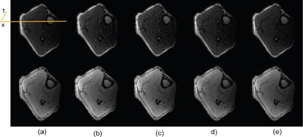
Spatial results: reconstruction comparison for calf muscle ASL perfusion data. (a) Reference, (b) PS Sparse, (c) SLR, (d) CS-PCA, (e) Proposed-KLR. Top: Frame 2; Bottom: Frame 7.
Fig. 7.
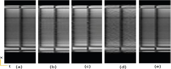
Calf muscle ASL perfusion data temporal variation of a cross section. (a) Reference, (b) PS Sparse, (c) SLR, (d) CS-PCA, (e) Proposed-KLR.
TABLE I.
RNMSE and Machine Time.
| Data | RNMSE | Machine Time (sec) | ||||||
|---|---|---|---|---|---|---|---|---|
|
| ||||||||
| PS Sparse | SLR | CS-PCA | Proposed-KLR | PS Sparse | SLR | CS-PCA | Proposed-KLR | |
|
| ||||||||
| Phantom | 0.0620 | 0.0580 | 0.0315 | 0.0210 | 122 | 148 | 104 | 720 |
| Cardiac cine | 0.0314 | 0.0394 | 0.0416 | 0.0214 | 125 | 102 | 85 | 676 |
| Muscle ASL | 0.822 | 0.651 | 0.0711 | 0.0261 | 28 | 32 | 52 | 68 |
| Myocardial ASL | 0.868 | 0.883 | 0.0983 | 0.0623 | 26 | 25 | 43 | 54 |
Fig. 8.
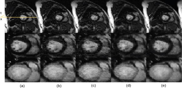
Spatial results: reconstruction comparison for myocardial ASL perfusion data. (a) Reference, (b) PS Sparse, (c) SLR, (d) CS-PCA, (e) Proposed-KLR. Top: Frame 2 Full FOV; Middle: Frame 2 ROI; Bottom: Frame 5 ROI.
Fig. 9.
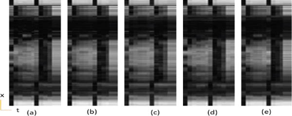
Myocardial ASL perfusion data temporal variation of a cross section, (a) Reference, (b) PS Sparse, (c) SLR, (d) CS-PCA, (e) Proposed-KLR.
Temporal intensity curves of Region of Interest (ROI) are typically of interest in ASL imaging. Figure 10 shows the temporal intensity curve of a particular ROI from the reference, CS-PCA and the proposed method. This shows the temporal curves from the proposed method follow the reference curve more consistently and precisely than the CS-PCA method.
Fig. 10.
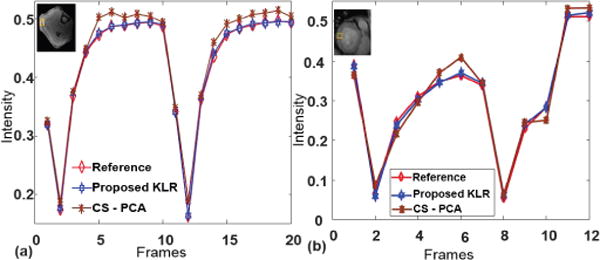
Intensity curve of an ROI in ASL perfusion (a) Muscle ASL data (b) Cardiac ASL data.
D. Cardiac Cine Results
Besides perfusion imaging, we also studied the usefulness of the proposed method in cardiac cine imaging using a set of cardiac cine data. The complex-valued multi-cycle cardiac cine data was simulated from human cardiac MR data acquired using a balanced SSFP sequence and single channel body coil on a 3T scanner with retrospective ECG-gating during a single breathhold and acquisition parameters TR = 3ms, matrix size = 200 × 256, field of view (FOV) = 273mm×350mm, spatial resolution = 1.36mm×1.36mm, slice thickness = 6mm. This data was then used to generate multiple time warps. Different heart rate variability and quasi-periodic spatial deformation along different cardiac cycle was obtained through thin plate spline mapping and nonlinear interpolation technique [61]. Each time warps were concatenated and a total of 40 frames were chosen representing about 3 cardiac cycle. It should be noted that the data in different cardiac cycles are not the same and such simulation has been used in [18]. Figure 11 shows the reconstruction results for the cine data with a reduction factor (R) of 5. The zoom-in views of the cardiac region show that the proposed method preserves the cardiac structures and intensity of myocardium better than the other methods. Figure 12 compares the temporal variation of the cross section along the yellow line indicated in the reference image. It demonstrates that the proposed method best preserves the temporal variations. Table I summarizes the RNMSEs and machine time for all test datasets. The qualitative reconstructions and quantitative measures signify that the proposed method outperforms the existing low-rank-based methods in these settings.
Fig. 11.
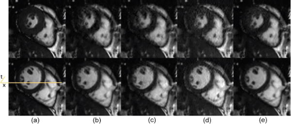
Spatial results: representative systolic and diastolic frames comparison for dynamic cardiac cine. (a) Reference, (b) PS Sparse, (c) SLR, (d) CS-PCA, (e) Proposed-KLR.
Fig. 12.

Cardiac cine temporal variation of a cross section. (a) Reference, (b) PS Sparse, (c) SLR, (d) CS-PCA, (e) Proposed-KLR.
However, when the number of frames is increased, as is usually the case in real-time cardiac cine imaging, the proposed method might not bring much advantage. To illustrate such limitation of the proposed method, we increase the frame rate of cardiac cine data in IV-D by about 3 times mimicking smoother temporal variation and a larger number of temporal frames. Retrospectively undersampled data using 1-D Cartesian sampling with a high reduction factor of 7.5 was then used in all reconstructions. From Fig. 13 and Fig. 14 we can see that the conventional PS-sparse method performs better than the proposed method. This is because 1) when the number of temporal frames in dynamic imaging is substantially increased with smoother temporal variations, the conventional approaches are able to find the low rank approximations of the dynamic image series; 2) the achievable reduction factor in the proposed method is limited by the need for low resolution images to perform kernel PCA. The reduction factor cannot be increased as much as PS-sparse with a large number of frames because the proposed method needs quite several navigator k-space lines to perform kernel PCA, while PS-sparse only needs very few lines for PCA.
Fig. 13.
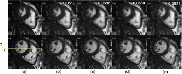
Spatial results: representative systolic and diastolic frames to illustrate limitation of the proposed method in the case of high frame rate and large numbers of frames. (a) Reference, (b) PS Sparse, (c) SLR, (d) CS-PCA, (e) Proposed-KLR. Numbers on top right of each column are respective RNMSE values.
Fig. 14.

Cardiac cine temporal variation of a cross section in the case of high frame rates and large number of frames. (a) Reference, (b) PS Sparse, (c) SLR, (d) CS-PCA, (e) Proposed-KLR.
V. Discussions
A. Relationship with Existing Methods
While several dynamic image reconstruction methods based on the low rank model have demonstrated success in accelerating dMRI with very high reduction factors, a large number of temporal frames are usually required to reveal the low rankness. Motivated by the fact that the kernel method is able to reveal some non-obvious features of signals, here we presented a kernel-based framework to expand the temporal signal of the image series from a low dimensional input space to high dimensional feature space such that the low rankness model still holds for the cases with few frames. Perfusion imaging is a dynamic MRI example with typically fewer frames, in which kernel-based framework shows improvement over existing methods. Such a framework opens up many possibilities to extend most existing reconstruction algorithms to new algorithms using manifold models. The proposed method is only one of possibilities, extending the low rank model to the nonlinear kernel PCA model.
B. Region of operation and Convergence
The performance of the proposed method depends on the choice of rank Q in feature space and the initial threshold value Sth. The choice of Q and threshold affect the tradeoff between the smoothness and details in the reconstructed images. Figure 15 shows the mean squared error for muscle and myocardial ASL data as a function of Q and Sth while keeping other parameters fixed. We can clearly see that the error changes with the parameters, but is consistent over a wide range, suggesting the method is insensitive to small changes of the parameters. The values of the parameters giving the least MSE have been used in the results.
Fig. 15.
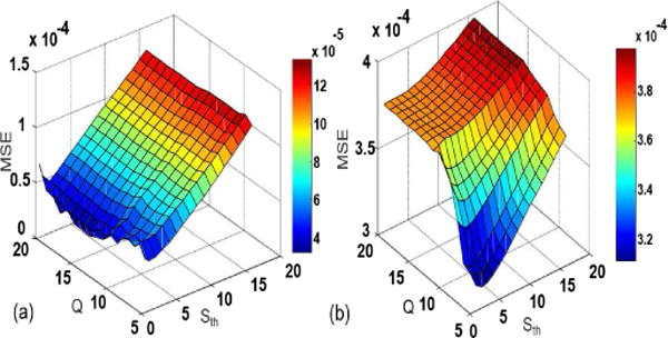
Region of operation test: MSE for different Q and threshold values. (a) muscle ASL perfusion data, (b) myocardial ASL perfusion data.
Figure 16 shows the performance of proposed method over different polynomial degrees d and constants c. Our experimental results show that the degree of order 3 gives the least MSE and the results are not sensitive significantly to constant c in the range of 100–1000. For better visualization, the MSE axis and the constant axis are shown in log scale in Fig. 16(a) and Fig. 16(b), respectively.
Fig. 16.
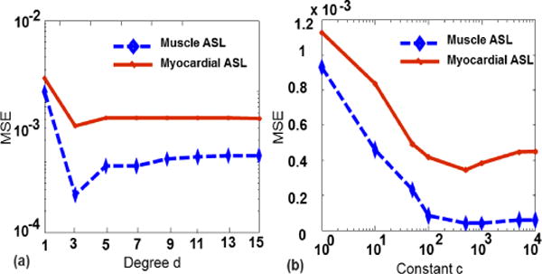
Performance analysis for different polynomial degree and constant.(a) MSE vs degree d, (b) MSE vs constant c.
Although the convergence of the proposed algorithm has not been proved theoretically due to different iterative parameters, our results have shown empirically that the proposed algorithm consistently converges. Figure 17 illustrates the convergence curve of the proposed method for different Q values keeping other parameters fixed.
Fig. 17.
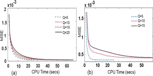
Convergence test: convergence rate for different Q (a) muscle ASL perfusion data, (b) myocardial ASL perfusion data.
C. Computational Complexity and Machine Time
The proposed method requires longer machine time than the competing methods due to the inherent extra operations in decomposition of the kernel matrix which increases with increase in numbers of training signals, and preimaging process which is not required in competing methods. It is important to note that the computation complexity of eigen-decomposition of the kernel matrix in Eq. (7) is O(T3) which only depends on the numbers of training data T (independent of the dimension of the feature space) [43], whereas the conventional low rank approximation costs O(MN2) for computation of the covariance matrix and O(N3) for singular value decomposition [62] which depends on the size of the image M and number of frames N. The increase in machine time is mainly attributed to the decomposition of kernel matrix and extra preimaging step which is not needed in other approaches.
D. Future Extensions
We present here a new kernel-based framework for dMRI reconstruction from sub-Nyquist acquisitions. The framework naturally motivates future studies on nonlinear sparsity models, and eventually combine nonlinear low rank and sparsity models using kernel method. The proposed method can also be integrated with existing parallel imaging techniques to further accelerate the data acquisition speed. Although our proposed method uses a single kernel for nonlinear low rank representation, multiple-kernel manifold models may be beneficial to application-specific dMRI reconstruction problems. Learning kernels from the undersampled data or data adaptive nonlinear dictionary learning instead of using generic kernels can be a challenging, yet interesting problem for future endeavors.
VI. Conclusion
In this paper we proposed a novel kernel-based framework for reconstructing dynamic MR images using manifold models. Within the framework, we extended the conventional low rank model to the feature space and developed a new method based on a kernel low-rank model. We have demonstrated that fewer nonlinear temporal basis than linear ones are needed to capture the temporal variations in dMRI. The method has shown its practical and successful application to the recovery of dynamic MR images from undersampled data, when existing low rank models fail, and its superior performance to the existing methods. It would be interesting to explore kernel extensions of other compressed-sensing based approaches in future studies.
Acknowledgments
This work is supported in part by the National Science foundation CBET-1265612, NSF CCF-1514403 and National Institute of Health R21EB020861.
We thank the anonymous reviewers for their comments and helping us to improve the quality of the paper significantly. We also thank Drs. Y. Wang (Cornell University), Z.-P. Liang (UIUC) and J. Zheng (Washington University) for helping with acquisition of different data sets.
Contributor Information
Ukash Nakarmi, Department of Electrical Engineering, University at Buffalo, NY, 14260, USA.
Yanhua Wang, School of Information and Electronics, Beijing Institute of Technology, Beijing, China.
Jingyuan Lyu, Department of Electrical Engineering, University at Buffalo, NY, 14260, USA.
Dong Liang, Paul C. Lauterbur Research Center for Biomedical Imaging, Shenzhen Institutes of Advanced Technology, Shenzhen, Guangdong 518055, China.
Leslie Ying, Department of Electrical Engineering, Department of Biomedical Engineering, University at Buffalo, NY, 14260, USA.
References
- 1.Liang Z-P, Lauterbur PC. An efficient method for dynamic magnetic resonance imaging. Medical Imaging, IEEE Transactions on. 1994;13(4):677–686. doi: 10.1109/42.363100. [DOI] [PubMed] [Google Scholar]
- 2.Madore B, Glover GH, Pelc NJ, et al. Unaliasing by fourier-encoding the overlaps using the temporal dimension (UNFOLD), applied to cardiac imaging and fMRI. Magnetic Resonance in Medicine. 1999;42(5):813–828. doi: 10.1002/(sici)1522-2594(199911)42:5<813::aid-mrm1>3.0.co;2-s. [DOI] [PubMed] [Google Scholar]
- 3.Liang Z-P. Spatiotemporal imaging with partially separable functions. Biomedical Imaging (ISBI), IEEE International Symposium on. 2007 Apr;:988–991. [Google Scholar]
- 4.Tsao J, Kozerke S. MRI temporal acceleration techniques. Journal of Magnetic Resonance Imaging. 2012;36(3):543–560. doi: 10.1002/jmri.23640. [DOI] [PubMed] [Google Scholar]
- 5.Tsao J, Boesiger P, Pruessmann KP. k-t BLAST and k-t SENSE: Dynamic MRI with high frame rate exploiting spatiotemporal correlations. Magnetic Resonance in Medicine. 2003;50(5):1031–1042. doi: 10.1002/mrm.10611. [DOI] [PubMed] [Google Scholar]
- 6.Jung H, Sung K, Nayak KS, Kim EY, Ye JC. k-t FOCUSS: A general compressed sensing framework for high resolution dynamic MRI. Magnetic Resonance in Medicine. 2009;61(1):103–116. doi: 10.1002/mrm.21757. [DOI] [PubMed] [Google Scholar]
- 7.Jung H, Ye JC, Kim EY. Improved k-t BLAST and k-t SENSE using FOCUSS. Physics in medicine and biology. 2007;52(11):3201. doi: 10.1088/0031-9155/52/11/018. [DOI] [PubMed] [Google Scholar]
- 8.Doneva M, Börnert P, Eggers H, Stehning C, Sénégas J, Mertins A. Compressed sensing reconstruction for magnetic resonance parameter mapping. Magnetic Resonance in Medicine. 2010;64(4):1114–1120. doi: 10.1002/mrm.22483. [DOI] [PubMed] [Google Scholar]
- 9.Ravishankar S, Bresler Y. MR image reconstruction from highly undersampled k-space data by dictionary learning. Medical Imaging, IEEE Transactions on. 2011;30(5):1028–1041. doi: 10.1109/TMI.2010.2090538. [DOI] [PubMed] [Google Scholar]
- 10.Wang Y, Ying L. Compressed sensing dynamic cardiac cine MRI using learned spatiotemporal dictionary. Biomedical Engineering, IEEE Transactions on. 2014;61(4):1109–1120. doi: 10.1109/TBME.2013.2294939. [DOI] [PubMed] [Google Scholar]
- 11.Bilgic B, Goyal VK, Adalsteinsson E. Multi-contrast reconstruction with bayesian compressed sensing. Magnetic Resonance in Medicine. 2011;66(6):1601–1615. doi: 10.1002/mrm.22956. [DOI] [PMC free article] [PubMed] [Google Scholar]
- 12.Chen L, Schabel MC, DiBella EV. Reconstruction of dynamic contrast enhanced magnetic resonance imaging of the breast with temporal constraints. Magnetic Resonance Imaging. 2010;28(5):637–645. doi: 10.1016/j.mri.2010.03.001. [DOI] [PMC free article] [PubMed] [Google Scholar]
- 13.Ji J, Lang T. Dynamic MRI with compressed sensing imaging using temporal correlations. Biomedical Imaging (ISBI), IEEE International Symposium on. 2008:1613–1616. [Google Scholar]
- 14.Gamper U, Boesiger P, Kozerke S. Compressed sensing in dynamic MRI. Magnetic Resonance in Medicine. 2008;59(2):365–373. doi: 10.1002/mrm.21477. [DOI] [PubMed] [Google Scholar]
- 15.Otazo R, Kim D, Axel L, Sodickson DK. Combination of compressed sensing and parallel imaging for highly accelerated first-pass cardiac perfusion MRI. Magnetic Resonance in Medicine. 2010;64(3):767–776. doi: 10.1002/mrm.22463. [DOI] [PMC free article] [PubMed] [Google Scholar]
- 16.Liang D, DiBella EV, Chen R-R, Ying L. k-t ISD: Dynamic cardiac mr imaging using compressed sensing with iterative support detection. Magnetic Resonance in Medicine. 2012;68(1):41–53. doi: 10.1002/mrm.23197. [DOI] [PMC free article] [PubMed] [Google Scholar]
- 17.Lustig M, Donoho D, Pauly JM. Sparse MRI: The application of compressed sensing for rapid MR imaging. Magnetic Resonance in Medicine. 2007;58(6):1182–1195. doi: 10.1002/mrm.21391. [DOI] [PubMed] [Google Scholar]
- 18.Zhao B, Haldar JP, Christodoulou AG, Liang Z-P. Image reconstruction from highly undersampled (k,t)-space data with joint partial separability and sparsity constraints. Medical Imaging, IEEE Transactions on. 2012;31:1809–1820. doi: 10.1109/TMI.2012.2203921. [DOI] [PMC free article] [PubMed] [Google Scholar]
- 19.Haldar J, Liang Z-P. Spatiotemporal imaging with partially separable functions: a matrix recovery approach. Biomedical Imaging (ISBI), International Symposium on. 2010 Apr;:716–719. [Google Scholar]
- 20.Lingala S, Hu Y, Dibella E, Jacob M. Accelerated dynamic MRI exploiting sparsity and low-rank structure: k-t SLR. Medical Imaging, IEEE Transactions on. 2011;30:1042–1054. doi: 10.1109/TMI.2010.2100850. [DOI] [PMC free article] [PubMed] [Google Scholar]
- 21.Otazo R, Candès EJ, Sodickson DK. Low-rank plus sparse matrix decomposition for accelerated dynamic MRI with separation of background and dynamic components. Magnetic Resonance in Medicine(Early view) 2014 doi: 10.1002/mrm.25240. [DOI] [PMC free article] [PubMed] [Google Scholar]
- 22.Tenenbaum JB, De Silva V, Langford JC. A global geometric framework for nonlinear dimensionality reduction. Science. 2000;290(5500):2319–2323. doi: 10.1126/science.290.5500.2319. [DOI] [PubMed] [Google Scholar]
- 23.Roweis ST, Saul LK. Nonlinear dimensionality reduction by locally linear embedding. Science. 2000;290(5500):2323–2326. doi: 10.1126/science.290.5500.2323. [DOI] [PubMed] [Google Scholar]
- 24.Donoho DL, Grimes C. Hessian eigenmaps: Locally linear embedding techniques for high-dimensional data. Proceedings of the National Academy of Sciences. 2003;100(10):5591–5596. doi: 10.1073/pnas.1031596100. [DOI] [PMC free article] [PubMed] [Google Scholar]
- 25.Belkin M, Niyogi P. Laplacian eigenmaps for dimensionality reduction and data representation. Neural computation. 2003;15(6):1373–1396. [Google Scholar]
- 26.Muller K, Mika S, Ratsch G, Tsuda K, Scholkopf B. An introduction to kernel-based learning algorithms. Neural Networks, IEEE Transactions on. 2001;12(2):181–201. doi: 10.1109/72.914517. [DOI] [PubMed] [Google Scholar]
- 27.Zhang Z, Zha H. Principal manifolds and nonlinear dimensionality reduction via tangent space alignment. Journal of Shanghai University (English Edition) 2004;8(4):406–424. [Google Scholar]
- 28.Cao L, Chua K, Chong W, Lee H, Gu Q. A comparison of PCA, KPCA and ICA for dimensionality reduction in support vector machine. Neurocomputing. 2003;55(12):321–336. support Vector Machines. [Google Scholar]
- 29.Borg I, Groenen PJ, Mair P. Applied Multidimensional Scaling Springer Science & Business Media. 2012 [Google Scholar]
- 30.Chen M, Silva J, Paisley J, Wang C, Dunson D, Carin L. Compressive sensing on manifolds using a nonparametric mixture of factor analyzers: Algorithm and performance bounds. Signal Processing, IEEE Transactions on. 2010;58(12):6140–6155. doi: 10.1109/TSP.2010.2070796. [DOI] [PMC free article] [PubMed] [Google Scholar]
- 31.Hegde C, Baraniuk RG. Signal recovery on incoherent manifolds. Information Theory, IEEE Transactions on. 2012;58(12):7204–7214. [Google Scholar]
- 32.Iwen MA, Maggioni M. Approximation of points on low-dimensional manifolds via random linear projections. Information and Inference. 2013;2(1):1–31. [Google Scholar]
- 33.Peyré G. Manifold models for signals and images. Computer Vision and Image Understanding. 2009;113(2):249–260. [Google Scholar]
- 34.Pourkamali Anaraki F, Hughes SM. Kernel compressive sensing. Image Processing (ICIP), 2013 20th IEEE International Conference on IEEE. 2013:494–498. [Google Scholar]
- 35.Qi H, Hughes S. Using the kernel trick in compressive sensing: Accurate signal recovery from fewer measurements. Acoustics, Speech and Signal Processing (ICASSP), 2011 IEEE International Conference on IEEE. 2011:3940–3943. [Google Scholar]
- 36.Poddar S, Jacob M. Dynamic MRI using smoothness regularization on manifolds (SToRM) Medical Imaging, IEEE Transactions on. 2016 Apr;35(4):1106–1115. doi: 10.1109/TMI.2015.2509245. [DOI] [PMC free article] [PubMed] [Google Scholar]
- 37.Schmidt JF, Santelli C, Kozerke S. MR image reconstruction using block matching and adaptive kernel methods. PloS one. 2016;11(4):1–14. doi: 10.1371/journal.pone.0153736. [DOI] [PMC free article] [PubMed] [Google Scholar]
- 38.Bhatia KK, Caballero J, Price AN, Hajnal JV, Rueckert D. Fast reconstruction of highly-undersampled dynamic MRI using random sampling and manifold interpolation. ISMRM. 2015 [Google Scholar]
- 39.Usman M, Atkinson D, Kolbitsch C, Schaeffter T, Prieto C. Manifold learning based ECG-free free-breathing cardiac cine MRI. Journal of Magnetic Resonance Imaging. 2015;41(6):1521–1527. doi: 10.1002/jmri.24731. [DOI] [PubMed] [Google Scholar]
- 40.Chung FR. Spectral Graph Theory Regional Conference Series in Mathematics. 1992;(92) [Google Scholar]
- 41.Bishop CM. Pattern Recognition and Machine Learning (Information Science and Statistics) Springer-Verlag New York, Inc; 2006. [Google Scholar]
- 42.Weinberger KQ, Sha F, Saul LK. Learning a kernel matrix for nonlinear dimensionality reduction. Twenty First International Conference on Machine Learning (ICML) 2004 [Google Scholar]
- 43.Mika S, Schölkopf B, Smola A, Müller KR, Scholz M, Rätsch G. Kernel PCA and de-noising in feature spaces. In: Kearns MS, Solla SA, Cohn DA, editors. Advances in Neural Information Processing Systems 11. Morgan Kaufmann; 1998. [Google Scholar]
- 44.Schölkopf B, Smola A, Müller K-R. Kernel principal component analysis. Artificial Neural Networks ICANN’97 Springer. 1997:583–588. [Google Scholar]
- 45.Zhou Y, Wang Y, Ying L. A kernel-based compressed sensing approach to dynamic MRI from highly undersampled data. Biomedical Imaging (ISBI), IEEE International Symposium on. 2013 Apr;:716–719. [Google Scholar]
- 46.Wang Y, Ying L. Undersampled dynamic magnetic resonance imaging using kernel principal component analysis. Engineering in Medicine and Biology Society (EMBC), Annual International Conference of the IEEE. 2014:1533–1536. doi: 10.1109/EMBC.2014.6943894. [DOI] [PubMed] [Google Scholar]
- 47.Nakarmi U, Wang Y, Lyu J, Ying L. Dynamic magnetic resonance imaging using compressed sensing with self-learned nonlinear dictionary (NL-D) Biomedical Imaging (ISBI), IEEE International Symposium on. 2015:331–334. [Google Scholar]
- 48.Pedersen H, Kozerke S, Ringgaard S, Nehrke K, Kim WY. k-t PCA: Temporally constrained k-t BLAST reconstruction using principal component analysis. Magnetic Resonance in Medicine. 2009;62(3):706–716. doi: 10.1002/mrm.22052. [DOI] [PubMed] [Google Scholar]
- 49.Wang R, Chen X. Manifold discriminant analysis. Computer Vision and Pattern Recognition, IEEE Conference on. 2009:429–436. [Google Scholar]
- 50.Belkin M, P N, Sindhwani V. Manifold regularization: A geometric framework for learning from examples. 2006 [Google Scholar]
- 51.Ham J, Lee DD, Mika S, Schlkopf B. A kernel view of the dimensionality reduction of manifolds. International Conference on Machine Learning (ICML) 2004 [Google Scholar]
- 52.Schölkopf B, Smola AJ. Learning with Kernels Cambridge: MIT Press. 2001 [Google Scholar]
- 53.Zheng WS, Lai J, Yuen PC. Penalized preimage learning in kernel principal component analysis. Neural Networks, IEEE Transactions on. 2010;21(4):551–570. doi: 10.1109/TNN.2009.2039647. [DOI] [PubMed] [Google Scholar]
- 54.Honeine P, Richard C. Preimage problem in kernel-based machine learning. IEEE Signal Processing Magazine. 2011;28(2):77–88. [Google Scholar]
- 55.Aharon M, Elad M, Bruckstein A. K-SVD: An algorithm for designing overcomplete dictionaries for sparse representation. Signal Processing, IEEE Transactions on. 2006;54(11):4311–4322. [Google Scholar]
- 56.Nguyen H, Patel VM, Nasrabadi NM, Chellappa R. Kernel dictionary learning. Acoustics, Speech and Signal Processing (ICASSP), 2012 IEEE International Conference on IEEE. 2012:2021–2024. [Google Scholar]
- 57.Donoho DL. De-noising by soft-thresholding. Information Theory, IEEE Transactions on. 1995 May;41(3):613–627. [Google Scholar]
- 58.Xu B, Spincemaille P, Chen G, et al. Fast 3D contrast enhanced MRI of the liver using temporal resolution acceleration with constrained evolution reconstruction. Magnetic Resonance in Medicine. 2013;69(2):370–381. doi: 10.1002/mrm.24253. [DOI] [PubMed] [Google Scholar]
- 59.Zheng J, An H, Coggan AR, et al. Noncontrast skeletal muscle oximetry. Magnetic Resonance in Medicine. 2014;71(1):318–325. doi: 10.1002/mrm.24669. [DOI] [PMC free article] [PubMed] [Google Scholar]
- 60.Northrup BE, McCommis KS, Zhang H, et al. Resting myocardial perfusion quantification with CMR arterial spin labeling at 1.5 T and 3.0 T. Journal of Cardiovascular Magnetic Resonance. 2008;10(1) doi: 10.1186/1532-429X-10-53. [DOI] [PMC free article] [PubMed] [Google Scholar]
- 61.Tsai Y, Ling H, Hu Y, et al. Thin plate spline technique for medical image deformation. Journal of medical and biological engineering) 2000;20:203–209. [Google Scholar]
- 62.Du Q, Fowler JE. Low-complexity principal component analysis for hyperspectral image compression. International Journal of High Performance Computing Applications. 2008;22(4):438–448. [Google Scholar]


