Spatial-Spectral Cube Matching Frame for Spectral CT Reconstruction

Abstract

Spectral computed tomography (CT) reconstructs the same scanned object from projections of multiple narrow energy windows, and it can be used for material identification and decomposition. However, the multi-energy projection dataset has a lower signal-noise-ratio (SNR), resulting in poor reconstructed image quality. To address this thorny problem, we develop a spectral CT reconstruction method, namely spatial-spectral cube matching frame (SSCMF). This method is inspired by the following three facts: i) human body usually consists of two or three basic materials implying that the reconstructed spectral images have a strong sparsity; ii) the same basic material component in a single channel image has similar intensity and structures in local regions. Different material components within the same energy channel share similar structural information; iii) multi-energy projection datasets are collected from the subject by using different narrow energy windows, which means images reconstructed from different energy-channels share similar structures. To explore those information, we first establish a tensor cube matching frame (CMF) for a BM4D denoising procedure. Then, as a new regularizer, the CMF is introduced into a basic spectral CT reconstruction model, generating the SSCMF method. Because the SSCMF model contains an L₀-norm minimization of 4D transform coefficients, an effective strategy is employed for optimization. Both numerical simulations and realistic preclinical mouse studies are performed. The results show that the SSCMF method outperforms the state-of-the-art algorithms, including the simultaneous algebraic reconstruction technique, total variation minimization, total variation plus low rank, and tensor dictionary learning.

1. Introduction

The spectral computed tomography (CT) (also called spectroscopic CT, multi-energy or color CT) has attracted continuous attentions because it has a great potential for tissue characterization, lesion detection and material decomposition [1, 2]. For example, the dual-energy CT (DECT), as the simplest and commercially available clinical spectral CT, has been employed for material differentiation [3], urinary calculi characterization [4], etc. Recently, thanks to the emergence and development of photon-counting detectors (PCDs), the multi-energy CT moves one step forward in practical applications. For example, the MARS (Medipix All Resolution System) research group developed a MARS-CT-3 scanner using three pairs of PCDs [5]. However, the charge sharing, Kescape, and fluorescence x-ray emission and re-absorption lead to corrupted spectral CT projection datasets with complicated noises [6]. This can decrease the signal-noise-ratio (SNR) of the projections and further comprise the reconstructed image quality. Thus, a primary task of spectral CT is to reconstruct accurate and clean images from the noisy projections. To address this intractable problem, lots of spectral CT reconstruction algorithms have been developed. In our opinion, all the methods employ some prior knowledge, and the knowledge can be divided into two categories: empirical-knowledge and prior-image-knowledge.

Regarding the empirical-knowledge based methods, they first convert the image into transform domain with a unified and image-independent transformation, and then focus on minimizing an L_0-norm or L₁-norm of the transform coefficients. Specifically, a satisfied image can be obtained by introducing man-made image characteristics as prior knowledge into the basic reconstruction model and optimizing the whole objection function. To address different problems in practical applications, different empirical-knowledge were reported, such as total variation (TV) [7], PRISM (prior rank, intensity and sparsity model) method [8], tensor-based nuclear norm [9], piecewise linear tight frame transform [10], total nuclear variation (TVN) [11], etc. Indeed, these reconstruction algorithms can obtain a satisfied result by enforcing the sparsity over a reconstructed image. Furtherly, the patch-based low-rank [1] , tensor nuclear norm (TNN) with TV [12], structure tensor TV [13] methods consider energy channel images similarity to formulate reconstruction model. However, image similarities in non-local spatial space are usually ignored among these methods. It can result in blurred edges, and finer structures are lost in the reconstructed images.

A representative group of prior-image-knowledge based methods are achieved by constructing a redundant dictionary from high quality images. This group can explore both image sparsity and similarity with a dictionary. They can be divided into two steps: dictionary training and image reconstruction. The first step is to train a redundant dictionary using images reconstructed by an analytic (e.g. FBP) or iterative (e.g. SART) algorithm. The second step is to reconstruct spectral images using the trained dictionary. In 2012, Zhao et al. applied a dual-dictionary learning (DDL) method for sparse-view spectral CT reconstruction [14]. Considering the image similarity among different energy channels, Zhang et al. introduced a tensor dictionary learning (TDL) into the spectral CT reconstruction [15]. To enhance the capability for clinical applications, very recently, Wu et al. incorporated an image gradient L₀-norm into the TDL (L₀TDL) framework for low-dose spectral CT [2]. Note that the final results depend on the image quality in the training process. The higher the quality of training image is, the better the reconstructed image is. Another group prior-image-knowledge based methods are realized by introducing a high quality spectral image into the optimized reconstruction model to constrain solution, such as spectral prior image constrained compressed sensing algorithm (spectral PICCS)[16], TV-TV and total variation spectral mean (TV-SM) methods [17]. In general, both of the two groups need high quality prior images. However, it might be impossible to obtain high quality prior images in practice. In addition, this type of reconstruction method can not consider image similarity within non-local spatial space.

About ten years ago, the Block Matching 3D (BM3D) was proposed for 2D image denoising by considering small image patch similarity within a searching window [18]. Then, it also obtained a great success in image deblurring [19], inpainting [20] and compression [21], etc. To address the volumetric image denoising issue, the BM3D was extended to BM4D and then it was applied to limited-angle MRI reconstruction [22]. Because the BM4D can accurately explore the nonlocal similarity of image cubes, it was applied to multispectral [23] and hyperspectral denoising [24] with a great success.

To handle the aforementioned spectral CT reconstruction issues, i.e., image edge blurring and finer structure losing in the empirical-knowledge based methods and difficulty in obtaining high quality prior images in the prior-image-knowledge based methods, we propose a spatial-spectral cube matching frame (SSCMF) to explore the spatial-spectral space similarity for spectral CT. Compared with the previous other tensor-based or multi-channel-based methods [15, 25, 26], the proposed SSCMF not only considers image structure similarity across spectral channels but also explores the non-local similarity of spectral image itself by clustering up a series of similar small cubes. The contributions are threefold. First, we establish a tensor cube matching frame based on the BM4D denoising procedure. Its insight can be easily considered as a regularizer. We thus call it cube matching frame (CMF) for convenience. Such a regularization term not only encodes the sparsity insights delivered by the traditional sparsity constraint, but also explores the similarities implied in a 3^rd tensor. Second, we sufficiently analyze the features of spectral images and introduce the CMF regularization term into the spectral CT reconstruction to further explore the image similarity and sparsity. This technique is named as spatial-spectral cube matching frame (SSCMF). Third, an effective denoising technique is employed to solve the 4D group coefficient L₀-norm minimization problem in the SSCMF model [27].

The rest of this paper is organized as follows. In section II, we establish the tensor CMF for BM4D. In section III, we construct the SSCMF model and adopt an effective denoising method for optimization. In section IV, both numerical simulations and real dataset experiments are performed to evaluate the proposed SSCMF method. In section V, we discuss some related issues and draw the conclusions.

2. BM4D Denoising Model

2.1. BM4D Algorithm

The BM4D was proposed as a volumetric nonlocal image denoising technique [22]. It can be considered as a natural extension of the state-of-the-art BM3D algorithm [19]. Similar to the BM3D algorithm, the BM4D algorithm can be implemented in three steps:

• i)Grouping similar volumetric cubes. The volumetric image cubes within a given image window share similar structures and they can be clustered to one group. These cubes in the same group can be further stacked as a 4D data array. During the course of grouping the cubes, the noise level σ of the volumetric image significantly affects the grouping accuracy[18].
• ii)Filtering. This consists of hard-thresholding filtering and collaborating filtering. The hard-thresholding filtering is used for image denoising by removing small groupwise spectrum coefficients in a 4D transform domain. An initial image can be recovered by performing the inverse transformation from 4D coefficients. The final denoised volumetric image can be obtained by the collaborating filtering.
• iii)Aggregation. The final denoised image cubes will be rearranged into the original corresponding locations by adopting a general weighting method for redundancy. To illustrate the effectiveness of data redundancy, the matrix representation of BM3D was introduced in [19]. To explore the volumetric data denoising and realize spectral CT reconstruction, we first provide the tensor cube frame for the BM4D

2.2. Tensor Cube Frame of BM4D

Let $\mathcal{X}\in {\mathcal{R}}^{N_W\times N_H\times N_D}$ be a 3^rd order tensor and ${\mathcal{x}}_j\in {\mathcal{R}}^{n_1\times n_2\times n_3}$ (n₁ ≪ N_W, n₂ ≪ N_H, n₃ ≪ N_D) be an extracted tensor cube, where j = 1,2,…,J and J=(N_w-n₁ + 1)(N_H – n₂ + 1) × (N_D –n₃ + 1). Assuming E_j represents the tensor cube extraction operation ${\mathcal{x}}_j$ can be expressed as

$${\mathcal{x}}_j=E_j(\mathcal{X}).$$ #(1)

For a tensor cube ${\mathcal{x}}_j$, we can determine a tensor searching window ${\mathcal{W}}_j\in {\mathcal{R}}^{N_1\times N_2\times N_3}$ (n₁ < N₁ < N_W, n₂ < N₂ < N_H, n₃ < N₃ < N_D). The process of determining a search window can considered as a special operation on $\mathcal{X}$. Let ${\mathcal{Z}}_j$ represents the operation of determining a search window,the searching window ${\mathcal{W}}_j$ can be expressed as

$${\mathcal{W}}_j={\mathcal{Z}}_j(\mathcal{X}).$$ #(2)

We extract R tensor cubes ${\mathcal{Y}}_{j,r}(1<r\le R)$ in the searching window tensor ${\mathcal{W}}_j$. All the extracted sensor cubes are stacked to form a 4^th order tensor as the j^th For simplicity, we assume that R is fixed.it assumed that,for each volume pixel in the searching window, there is atleast one cube that entersin the group and contains the volumetric pixel. ${\mathcal{Y}}_{j,r}$ can expressed as

$${\mathcal{Y}}_{j,r}={\epsilon }_{j,r}\left({\mathcal{W}}_j\right),$$ #(3)

where ε_j,r represents the r^th tensor cube extraction operation from the j^th searching window.infact,the BM4D modeling can be considered as a special form of the 4d decorrelating transform.it can be realized by a combination of separable 3D intrablock and 1D interblock transforms. Let Φ(·)and Ψ(·) be the 3D interblock and 1D intrablock transforms,repectively. The 3D transform coefficient ${\mathcal{G}}_{j,r}$ of ${\mathcal{Y}}_{j,r}$ can be written as

$${\mathcal{G}}_{j,r}=\mathbf{\Phi }\left({\mathcal{Y}}_{j,r}\right).$$ #(4)

There, the 3D coefficients of the j^th group can be written as ${\mathcal{G}}_j=\left({\mathcal{G}}_{j,1},{\mathcal{G}}_{j,2},\dots ,{\mathcal{G}}_{j,R}\right)$. We apply the 1D interblock transformation to ${\mathcal{G}}_j$ and the 4D spectrum of this group ${\mathcal{w}}_j$ can be written as

$$\begin{gathered} {\mathcal{w}}_j=\mathbf{\Psi }\left({\mathcal{G}}_j\right)=\mathbf{\Psi }\left({\mathcal{G}}_{j,1},{\mathcal{G}}_{j,2},\dots ,{\mathcal{G}}_{j,R}\right)=\mathbf{\Psi }\left(\mathbf{\Phi }\left({\mathcal{Y}}_{j,1}\right),\mathbf{\Phi }\left({\mathcal{Y}}_{j,2}\right),\dots ,\mathbf{\Phi }\left({\mathcal{Y}}_{j,R}\right)\right) \\ =\mathbf{\Psi }\mathbf{\Phi }\left({\mathcal{Y}}_{j,1},{\mathcal{Y}}_{j,2},\dots {\mathcal{Y}}_{j,R}\right)=\mathbf{\Psi }\mathbf{\Phi }\left({\epsilon }_{j,1}\left({\mathcal{Z}}_j(\mathcal{X})\right),{\epsilon }_{j,2}\left({\mathcal{Z}}_j(\mathcal{X})\right),\dots ,{\epsilon }_{j,R}\left({\mathcal{Z}}_j(\mathcal{X})\right)\right). \end{gathered}$$ #(5)

Now, let ${\mathcal{E}}_j$ be (ε_j,1,ε_j,2,…,ε_j,R). Eq. (5) can be written as

$${\mathcal{w}}_j=\mathbf{\Psi }\mathbf{\Phi }\left[\left({\epsilon }_{j,1},{\epsilon }_{j,2},\dots ,{\epsilon }_{j,R}\right){\mathcal{Z}}_j(\mathcal{X})\right]=\mathbf{\Psi }\mathbf{\Phi }\left({\epsilon }_j\left({\mathcal{Z}}_j(\mathcal{X})\right)\right).$$ #(6)

Here, in order to better understand the process of the BM4D, ψ is denoted as a 4D analysis operator and it equal to ΨΦ. Thus, Eq. (6) can be simplified as

$${\mathcal{w}}_j=\mathit{\psi }\left({\mathcal{E}}_j\left({\mathcal{Z}}_j(\mathcal{X})\right)\right).$$ #(7)

Note that Eq. (6) only considers a group constructed from the j^th searching window. A set of all groupwise coefficients Ω of tensor $\mathcal{X}$ can be expressed as following

$$\mathbf{\Omega }(\mathcal{X})=\left(\begin{array}{c}{\mathcal{w}}_1\\ ⋮\\ {\mathcal{w}}_J\end{array}\right).$$ #(8)

The synthesis transform of BM4D model can be similarly derived First, the inverse intrablock 1D transform and 3D transforms are applied to each tensor group spectrum ${\mathcal{w}}_j$. Then the obtained tensor cubes estimation are rearranged into their corresponding original position. The estimated tensor group from the j^th group spectrum can be denoted as ${\widehat{\mathcal{Z}}}_j(\mathcal{X})={\mathcal{E}}_j^{-1}\mathit{\vartheta }\left({\mathcal{w}}_j\right)$, where ϑ is the BM4D synthesis operation and ${\mathcal{E}}_j^{-1}$ represents the inverse of extraction operation ${\mathcal{E}}_j$ with appropriate weighting for redundancy. The final image can be further obtained by a weighting strategy i.e., the gropuwise estimation using weights α_j > 0 therefore, tensor $\mathcal{X}$ can be recovered as the following expression

$$\widehat{\mathcal{X}}={\mathit{\alpha }}^{-\mathbf{1}}\left(\begin{array}{c}{\mathit{\alpha }}_1{\mathcal{E}}_1^{-1}\mathit{\vartheta }\left({\mathcal{w}}_1\right)\\ ⋮\\ {\mathit{\alpha }}_J{\mathcal{E}}_J^{-1}\mathit{\vartheta }\left({\mathcal{w}}_J\right)\end{array}\right),$$ #(9)

where

$$\mathit{\alpha }={\displaystyle \sum _{j=1}^J}{\mathit{\alpha }}_j{\displaystyle \sum _{E_j(\mathcal{X})\in \mathcal{E}\left({\mathcal{Z}}_j(\mathcal{X})\right)}}{\mathcal{Z}}_j{}^T{\mathcal{Z}}_j$$

is a weighting tensor. if the u^th volume element of $\mathcal{X}$ belongs to the j^th tensor cube, the value of corresponding location on ${\mathcal{Z}}_j{}^T{\mathcal{Z}}_j$ would be 1 and otherwise it woul be 0. Therefore, the ${\sum }_{E_j(\mathcal{X})\in {\mathcal{E}}_{j,r}({\mathcal{Z}}_j(\mathcal{X}))}{\mathcal{Z}}_j{}^T{\mathcal{Z}}_j$ can indicate the number of cubes in the j^th group containing u^th tensor element.

2.3. Tensor frame Interpretation of BM4D

For a given group ${\mathcal{E}}_j\left({\mathcal{Z}}_j(\mathcal{X})\right)$, the 4D analysis operator ψ can transform it into the coefficient ${\mathcal{w}}_j$. In contrast, the BM4D synthesis operator ϑ can transform the group coefficient ${\mathcal{w}}_j$ into the corresponding tensor group ${\widehat{\mathcal{E}}}_j\left({\mathcal{Z}}_j(\mathcal{X})\right)$. The synthesis operator ϑ can be treated as an inverse transform of the analysis operartor ψ, i.e., ${\mathcal{E}}_j\left({\mathcal{Z}}_j(\mathcal{X})\right)=\mathit{\vartheta }\left(\mathit{\psi }\left({\mathcal{E}}_j\left({\mathcal{Z}}_j(\mathcal{X})\right)\right)\right)$. Again, the product ϑ and ψ can be expressed as

$$\mathit{I}=\mathit{\vartheta }\mathit{\psi },$$ #(10)

where I stands for the identify transform. However,an independent tensor group ${\mathcal{E}}_j\left({\mathcal{Z}}_j(\mathcal{X})\right)$ is considered in the above analysis,and our goal is to recover the whole tensor $\mathcal{X}$ from overlapped groups ${\left({\mathcal{E}}_1\left({\mathcal{Z}}_1(\mathcal{X})\right),\dots ,{\mathcal{E}}_J\left({\mathcal{Z}}_J(\mathcal{X})\right)\right)}^T$. Considering the weight coefficient tensor α, then the tensor $\mathcal{X}$ can be further recovered

$$\widehat{\mathcal{X}}={\mathit{\alpha }}^{-\mathbf{1}}\left(\begin{array}{c}{\mathit{\alpha }}_1{\mathcal{E}}_1^{-1}\mathit{\vartheta }\mathit{\psi }{\mathcal{E}}_1\left({\mathcal{Z}}_1(\mathcal{X})\right)\\ ⋮\\ {\mathit{\alpha }}_J{\mathcal{E}}_J^{-1}\mathit{\vartheta }\mathit{\psi }{\mathcal{E}}_J\left({\mathcal{Z}}_J(\mathcal{X})\right)\end{array}\right),$$ #(11)

which is in consisitent with Eq. (9).it is necessary to point out that the weight coefficient tensor α can be changed with respect to the image noise level σ. This means different noise may result im dofferent weight coefficient tensors.

3. Spectral CT Reconstruction based on spatial-spectral CMF

3.1. Spectral CT Imaging Model

Considering the noise in the projection datasets, the acquired or observed data forward model of the conventional CT for fan-beam scanning geometry van be approximated as a discretized linear system

$$\mathit{p}=\mathcal{A}\mathit{f}+\mathit{\eta },$$ #(12)

where $\mathit{f}\in {\mathcal{R}}^N$ (N = N_w × N_H) represents the vectorized 2D image, $\mathit{p}\in {\mathcal{R}}^T$ (T = T₁ × T₂) represents the measurements, T₁ and T₂ are respectively the view and detector numbers, $\mathcal{A}\in {\mathcal{R}}^{N\times T}$ is the CT projection matrix and $\mathit{\eta }\in {\mathcal{R}}^T$ stands for projection noise. Because the matrix $\mathcal{A}$ is huge, Eq. (12) can not be solved directly by adopting a matrix inverse technique due to the memory limitation Alternatively, it can be iteratively solved in terms of the following minimization problem

$$\underset{\mathit{f}}{\mathrm{argmin}}\frac{1}{2}\Vert \mathit{p}-\mathcal{A}\mathit{f}{\Vert }_2^2,$$ #(13)

where ‖.‖ represents the L₂ norm Eq. (13) involves the linear programming problem,which can be updated with the ART or SART methods. Methods [28] To further optimize the result of Eq. (13), a regularization of prior knowledge can be introduced into Eq. (13) Therefore, we have

$$\underset{\mathit{f}}{\mathrm{argmin}}\frac{1}{2}\Vert \mathit{p}-\mathcal{A}\mathit{f}{\Vert }_2^2+\tau \mathit{R}(\mathit{f}).$$ #(14)

Note that Eq. (14) consisits of two terms: data fidelity term $\frac{1}{2}\Vert \mathit{p}-\mathcal{A}\mathit{f}{\Vert }_2^2$ and regularization term R(f), and τ > 0 is a parameter to balance the data fidelity and regularization terms. For the regularization term R(f),it can be chosen as TV [29,30] wavelet frame [31], image gradient L_0-norm [32], low-rank [33],etc.

For the multi-energy CT, multiple projection datasets can be obtained with one scan. This means we can reconstruct multiple energy-dependent images of the same object using different projection datasets. Let u be the number of energy channels. Similar to Eq. (13), spectral CT reconstruction can be modeled as

$$\underset{\mathcal{F}}{\mathrm{argmin}}\left({\displaystyle \sum _{s=1}^S}\frac{1}{2}{\Vert {\mathit{p}}_s-\mathcal{A}{\mathit{f}}_s\Vert }_2^2\right)+\tau \mathit{R}(\mathcal{F}),$$ #(15)

where ${\mathit{f}}_s\in {\mathcal{R}}^N$ (s = 1,2,⋯,S) is a vectorized image of the s^th energy channel of a 3^rd order tensor $\mathcal{F}\in {\mathcal{R}}^{N_W\times N_H\times S}$, and the projection ${\mathit{p}}_s\in {\mathcal{R}}^T$ is a coloumn of $\mathit{P}\in {\mathcal{R}}^{N\times S}$. The first term of Eq. (15), (i.e., ${\sum }_{s=1}^S\frac{1}{2}{\Vert {\mathit{p}}_s-\mathcal{A}{\mathit{f}}_S\Vert }_2^2$) can be considered as data fidelity term for the multi-energy CT and it is formulated with summation of data fidelity error from all energy channels.

3.2. Spatial-spectral CMF for Spectral CT

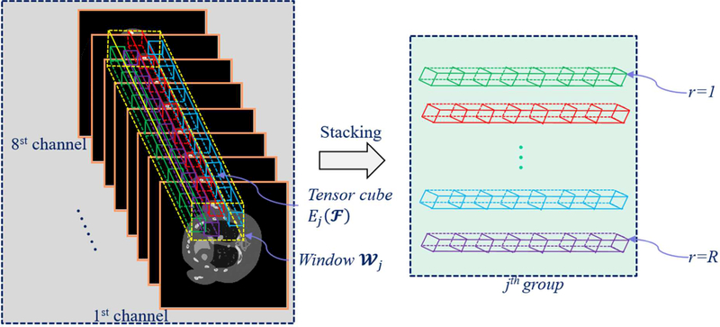
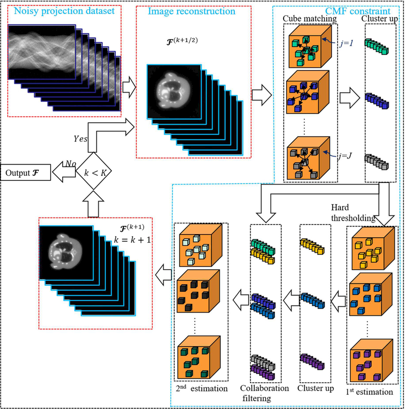
For the spectral CT, there are some facts: i) from the aspects of material decomposition, patients usually consist of two or three basic materials, i.e., soft tissue, bone and water. Thus, the constructed spectral images have a strong sparsity in material composition; ii) the same basic material components in a single channel have similar intensity and structures. Different material components within the same energy channel share similar structural information; iii) multi-energy projection datasets are collected from the same patient by using different energy windows. Although images reconstructed from different energy channels have different attenuation coefficients, they share the same physical structures; iv) charge sharing, K-escape, and fluorescence x-ray emission and re-absorption can cause severe noise in the reconstructed images. Considering the advantages of CMF in characterizing 3D image similarity and reducing noise, the CMF as a regularizer is introduced into the spectral CT reconstruction to generate a spatial-spectral CMF (SSCMF) reconstruction method. Fig. 1 demonstrates the process of grouping which is a key procedure in the SSCMF method. We extract similar tensor cubes within a given spatial-spectral searching window and then stack them as the j^th group. To clarify the procedure of SSCMF algorithm, Fig. 2 shows flowchart for the whole iteration. The proposed SSCMF method can be divided into two steps: image reconstruction and CMF constraint. For image reconstruction, we adopt the SART to perform back projection. In the CMF constraint step, first, the images reconstructed by the SART are grouped and clustered as 4D arrays. Then, the noises in these 4D data arrays can be suppressed by the hard-thresholding operation. This process can be considered as the 1st estimation. To enhance the denoising capability of the CMF, we perform the collaborative filtering on the original signal and initial estimation, which can be called as the 2nd estimation.

Fig.1.

Illustration of grouping spatial-spectral cubes.

Fig.2.

The flowchart of SSCMF method.

3.3. SSCMF Model

Mathematically speaking, the SSCMF model can be constructed as follow

$$\underset{\mathcal{F}}{\mathrm{argmin}}\left\{\left({\displaystyle \sum _{s=1}^S}\frac{1}{2}{\Vert {\mathit{p}}_s-\mathcal{A}{\mathit{f}}_s\Vert }_2^2\right)+\tau \Vert \mathbf{\Omega }(\mathcal{F}){\Vert }_0\right\},$$ #(16)

where ‖.‖ represents the L₀ norm regularization term of the spatial –spectral cube 4D transform coefficients. Since this model contains the quasi L_0-norm it makes Eq.(16) an NP-hard problem Here,we employ a strategy in [27] to minimize eq. (16) which can be divided into two steps:

$$\{\begin{array}{c}{\mathcal{F}}^{(k+1/2)}=\underset{\mathcal{F}}{\mathrm{argmin}}\left({\displaystyle \sum _{s=1}^5}\frac{1}{2}{\Vert {\mathit{p}}_s-\mathcal{A}{\mathit{f}}_s\Vert }_2^2\right)+\frac{\lambda }{2}{\Vert \mathcal{F}-{\mathcal{F}}^{(k)}\Vert }_F^2,\\ {\mathcal{F}}^{(k+1)}=\underset{\mathcal{F}}{\mathrm{argmin}}{\Vert \mathcal{F}-{\mathcal{F}}^{(k+1/2)}\Vert }_F^2+\tau \Vert \mathbf{\Omega }(\mathcal{F}){\Vert }_0,\end{array}$$ #(17a)#(17b)

where λ is acoupling parameter and ‖.‖_F represents the tensor frobenius norm Eqs. (17a) and (17b) can be called as observation fidelity and model fidelity steps, respectively. Especially, different forward system matrix $\mathcal{A}$ means different imaging problems. For example, when $\mathcal{A}$ means different imaging problems. For example ,when A corresponds a bluring matrix, Eq. (17a) is to update the current intermediate tensor image ${\mathcal{F}}^{(k+1/2)}$ so that it can be better agree with observation matrix P in the image debluring problem [27]. The regularization parameter λ is introduced into Eq(17a) to determine the degree of agreement between ${\mathcal{F}}^{(k+1/2)}$ and P. Eq. (17b) achieves an accurate update which can conform with the prior image model or structure as enforced by the penalty function $\Vert \mathbf{\Omega }(\mathcal{F}){\Vert }_0$. For the spectral data fidelity term, because the update of each energy channel is independent, Eq (17a) can be rewritten as

$${\mathcal{F}}^{\left(k+\frac{1}{2}\right)}=\underset{\mathcal{F}}{\mathrm{argmin}}{\displaystyle \sum _{s=1}^S}\left(\frac{1}{2}{\Vert {\mathit{p}}_s-\mathcal{A}{\mathit{f}}_S\Vert }_F^2+\frac{\lambda }{2}{\Vert {\mathit{f}}_s-{\mathit{f}}_s^{(k)}\Vert }_2^2\right).$$ #(18)

The update of ${\mathcal{F}}^{\left(\mathit{k}+\frac{\mathbf{1}}{\mathbf{2}}\right)}$ can be achieved by separetly updating all energy channel image f_s(s = 1,…,S). Therefore, Eq. (18) is equivalent to

$${\mathit{f}}_s^{\left(k+\frac{1}{2}\right)}=\underset{{\mathit{f}}_s}{\mathrm{argmin}}\frac{1}{2}{\Vert {\mathit{p}}_s-\mathcal{A}{\mathit{f}}_s\Vert }_2^2+\frac{\lambda }{2}{\Vert {\mathit{f}}_s-{\mathit{f}}_s^{(k)}\Vert }_2^2,(s=1,\dots ,S).$$ #(19)

To determine the minimization point of f_s,the derivate of Eq. (19) should be equivalent to zero. We have,

$$-{\mathcal{A}}^T\left({\mathit{p}}_s-\mathcal{A}{\mathit{f}}_s\right)+\lambda \left({\mathit{f}}_s-{\mathit{f}}_s^{(k)}\right)=0,(s=1,\dots ,S).$$ #(20)

which can be simplified as

$$\left({\mathcal{A}}^T\mathcal{A}+\lambda \mathit{I}\right){\mathit{f}}_s={\mathcal{A}}^T{\mathit{p}}_S+\lambda {\mathit{f}}_S^{(k)}.(s=1,\dots ,S)$$ #(21)

Eq. (21) is equivalent to

$$\left({\mathcal{A}}^T\mathcal{A}+\lambda \mathit{I}\right){\mathit{f}}_s={\mathcal{A}}^T{\mathit{p}}_s+\lambda {\mathit{f}}_s^{(k)}+{\mathcal{A}}^T\mathcal{A}{\mathit{f}}_s^{(k)}-{\mathcal{A}}^T\mathcal{A}{\mathit{f}}_s^{(k)},(s=1,\dots ,S)$$ #(22)

$$\left({\mathcal{A}}^T\mathcal{A}+\lambda \mathit{I}\right){\mathit{f}}_s=\left({\mathcal{A}}^T\mathcal{A}+\lambda \mathit{I}\right){\mathit{f}}_s^{(k)}+{\mathcal{A}}^T\left({\mathit{p}}_s-\mathcal{A}{\mathit{f}}_s^{(k)}\right).(s=1,\dots ,S)$$ #(23)

Therefore, ${\mathit{f}}_s^{\left(k+\frac{1}{2}\right)}$ can be updated as

$${\mathit{f}}_s^{\left(k+\frac{1}{2}\right)}={\mathit{f}}_s^{(k)}+\beta {\left({\mathcal{A}}^T\mathcal{A}+\lambda \mathit{I}\right)}^{-1}{\mathcal{A}}^T\left({\mathit{p}}_s-\mathcal{A}{\mathit{f}}_s^{(k)}\right),(s=1,\dots ,S),$$ #(24)

where β = 1 and it can be any other relaxation factor in the range of (0,2). Eq. (21) indicates that λ only affects the iteration step. Considering Eq (24) as the solution of Eq. (17a), λ = 0 becomes a legal regularization parameter for a unique solution. In this case, Eq. (24) is degraded as the SART method [34]. Thus, λ is set as zero in this work.

The first term ${\Vert \mathcal{F}-{\mathcal{F}}^{(k+1/2)}\Vert }_F^2$ of Eq. (17b) can be considered as the data fidelity to balance the final estimation ${\mathcal{F}}^{(k+1)}$ and the current estimation ${\mathcal{F}}^{(k+1/2)}$. The regularization term $\Vert \mathbf{\Omega }(\mathcal{F}){\Vert }_0$ enforces the L₀-norm sparse constraint over the 4D tensor coefficients to suppress noise by removing small coefficients in the 4D transform domain.considering Eqs.(7) and (8), Eq. (17b) is equivalent to

$${\mathcal{F}}^{(k+1)}=\underset{\mathcal{F}}{\mathrm{argmin}}{\Vert \mathcal{F}-{\mathcal{F}}^{\left(k+\frac{1}{2}\right)}\Vert }_F^2+\tau {\Vert \mathit{\psi }\left(\begin{array}{c}{\mathcal{E}}_1\left({\mathcal{Z}}_1(\mathcal{F})\right)\\ ⋮\\ {\mathcal{E}}_J\left({\mathcal{Z}}_J(\mathcal{F})\right)\end{array}\right)\Vert }_0.$$ #(25)

Substituting Eq. (10) into Eq .(11) and then Eq. (25) becomes

$${\mathcal{F}}^{(k+1)}=\underset{\mathcal{F}}{\mathrm{argmin}}{\Vert \mathcal{F}-{\mathcal{F}}^{\left(k+\frac{1}{2}\right)}\Vert }_F^2+\tau {\Vert \left(\begin{array}{c}\mathit{\psi }{\mathcal{E}}_1{\mathcal{Z}}_1\\ ⋮\\ \mathit{\psi }{\mathcal{E}}_J{\mathcal{Z}}_J\end{array}\right)\mathcal{F}\Vert }_0,$$ #(26)

which can be further written as

$${\mathcal{F}}^{(k+1)}=\underset{\mathcal{F}}{\mathrm{argmin}}{\Vert \mathcal{F}-{\mathcal{F}}^{\left(k+\frac{1}{2}\right)}\Vert }_F^2+\tau \Vert \mathit{\varrho }(\mathcal{F}){\Vert }_0,$$ #(27)

where $\mathit{\varrho }=\left(\begin{array}{c}\mathit{\psi }{\mathcal{E}}_1{\mathcal{Z}}_1\\ ⋮\\ \mathit{\psi }{\mathcal{E}}_J{\mathcal{Z}}_J\end{array}\right)$. The problem of Eq (27) can be treated as a denoising with to solve such a problem with an analysis prior defined over the tensor frame shrinkage algorithm [36].In this work, we employ a typical technology (i.e., hard-thresholding method [36] to solve Eq. (27). The solution can be given as

$${\mathcal{F}}^{(k+1)}={\mathit{\alpha }}^{-1}{\mathit{\varrho }}^{-1}\lfloor \mathit{\varrho }{\left({\mathcal{F}}^{\left(k+\frac{1}{2}\right)}\right)\rfloor }_{\tau },$$ #(28)

where ϱ⁻¹ represents the inverse operator of the ϱ with appropriate weighting for redundancy. The operator ⌊⋅⌋_τ denotes the hard thresholding operation and it can be calculated as [36]

$${\lfloor \mathit{\varrho }\left({\mathcal{F}}^{\left(k+\frac{1}{2}\right)}\right)\rfloor }_{\tau }=\{\begin{array}{ll}0,\hfill & \mathit{\varrho }\left({\mathcal{F}}^{\left(k+\frac{1}{2}\right)}\right)<\sqrt{\tau }\hfill \\ \mathit{\varrho }\left({\mathcal{F}}^{\left(k+\frac{1}{2}\right)}\right),\hfill & \mathit{\varrho }\left({\mathcal{F}}^{\left(k+\frac{1}{2}\right)}\right)\ge \sqrt{\tau }\hfill \end{array}.$$ #(29)

It is necessary to emphasize that Eq. (29) can be implemented by the BM4D denoising algorithm, which is formulated using the frame notation in [22]. For our proposed reconstruction algorithm, the frame shrinkage step Eq. (29) is treated as an approximate solution for Eq. (17b). Therefore, Eq. (17b) will be updated by a BM4D-based denoising for spectral CT images. Our algorithm mainly explores the similarity of spatial-spectral information by utilizing the cube matching frame regularization and its workflow is summarized as Algorithm I.

Algorithm I.

SSCMF

Input: λ,τ,β,σ,P;

1: Initialization of $\mathcal{F}\leftarrow \mathbf{0}$, k = 0

2: repeat

3: for s: = 1,2, ⋯,S do

4: Updating ${\mathit{f}}_s^{(k+1/2)}$ by SART

5: end for

6: Generating frames ψ and ϑ using the ${\mathcal{F}}^{(k+1/2)}$;

7: Updating ${\mathcal{F}}^{(k+1)}$ using Eq. (28);

8: Applying positive constraint over ${\mathcal{F}}^{(k+1)}$;

9: k = k + 1;

10: until convergence

Output: Reconstructed spectral CT image $\mathcal{F}$

In the Algorithm I, the model fidelity 6–7 steps correspond to the BM4D denoising process of image ${\mathit{f}}_S^{(k+1/2)}$. They are implemented by adopting a highly available online optimized BM4D denoising toolbox [22] (http://www.cs.tut.fi/~foi/GCF-BM3D/). Eq. (28) is implemented with a 4D transform shrinkage followed by the wiener collaborative filtering.Here, the coefficient shrinkage Eq. (29) is implemented by a hard thresholding filtering with the controlling parameter τ in our numerical simulations and preclinical experiments ,the cube size is 4 × 4 × 4 and the sliding step is 3. Other parameter setting and transform selection are the same as those in the BM4D denosing toolbox (http://www.cs.tut.fi/~foi/GCF-BM3D/).

4. Experiments

To evaluate the performance of our SSCMF method, simultaneous algebratic reconctruciton technique (SART), total variation minimization (TVM), total variation plus low rank (TV+LR)[8], and tensor dictionary learning (TDL)[15] algorithms are selected and implemented for comparison. Both numerical simulations and preclinical spectral datasets are employed for stopped after 50 iterations. The relaxation factor β is fixed as 0.03 and other parameters are evaluation. For all the iterative methods, the initial images are set as zero and all of them are optimized and summarized as in Table 1.

Table 1.

Reconstruction parameters for both numerical simulations and preclinical datasets.

	Photon number	σ	τ
Mouse thorax phantom	2×104	0.016	12
	5×103	0.05	10
Preclinical dataset		0.02	0.35

4.1. Mouse Thorax Phantom Study

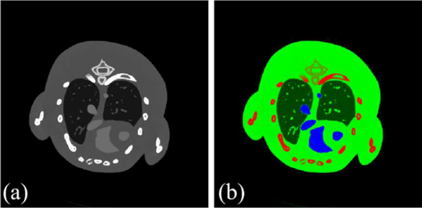
A simulated mouse thorax phantom is employed, containing three basic materials: soft tissue, bone, and iodine (Fig. 3). As shown in Fig. 3, 1.2% iodine is injected into the mouse thorax phantom as contrast agent. A polychromatic 50KVp x-ray source is assumed, and it is divided into eight different energy channels: [16, 22) keV, [22, 25) keV, [25, 28) keV, [28, 31) keV, [31, 34) keV, [34, 37) keV, [37, 41) keV, and [41, 50) keV. The PCD used in the experiment contains 512 detector elements, and each element covers a length of 0.1mm. Regarding the scanning geometry, the distances from source to rotation center and PCD are 132mm and 180mm, respectively. 640 projections are uniformly collected over a full scan. Each reconstructed energy channel image consists of 512×512 pixels, and each pixel covers an area of 0.075×0.075 mm². The photon number of each x-ray path is set as 2×10⁴, and Poisson noise is added in to the received photon number.

Fig 3.

The mouse thorax phantom. (a) is the 1st channel image in [0, 3] cm⁻¹ reconstructed by the SART with full-scan noise-free projections. (b) is the merged color image where green, red and blue stand for soft tissue, bone and iodine, respectively.

a). Reconstruction Results

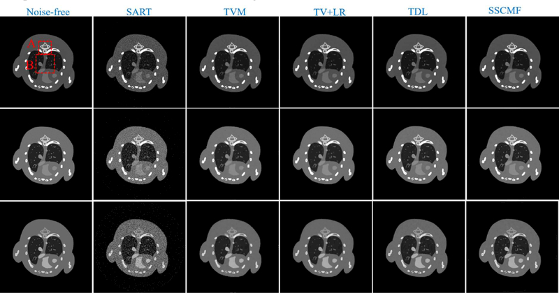
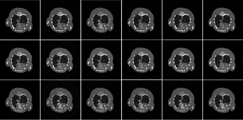
To compare the performances of all algorithms in spectral CT reconstruction, parameters in all algorithms are optimized, and their best results are selected for comparison and analysis. Fig. 4 shows the reconstructed images of three representative energy channels (1^st, 4^th and 8^th). One can see that the SSCMF algorithm always obtain higher quality images compared with other competitors. More specifically, the SSCMF method outperforms other algorithms in edge preservation and finer structure recovery. This point is further confirmed by two magnified region of interests (ROIs) A (bony structure) and B (soft tissue) in Fig. 5. It can be observed that images reconstructed by using the SART have the strongest noise. The TVM, TV+LR and TDL methods can reduce noise to a certain extent, but the profiles of reconstructed images are not clearer. In contrast, the SSCMF method has an excellent performance in noise reduction as well as image edge preservation. Fig. 6 plots representative profiles along the yellow line in bony structure A in Fig. 5. From Fig. 6, one can infer that the profiles of SSCMF method are closer to the ground truths compared with the TVM, TV+LR and TDL algorithms.

Fig. 4.

Reconstructed results of three representative energy-channel images. The 1st to 3rd row images correspond to the 1st, 4th and 8th channels, and their display windows are [0, 3], [0, 1.2] and [0, 0.8] cm⁻¹, respectively.

Fig. 5.

Magnified ROIs A (bony structure) and B (soft tissue) in Fig. 4.

Fig. 6.

Representative profiles along the yellow line in bony ROI A in Fig. 5. (a), (b) and (c) are for 1, 4 and 8 channels, respectively.

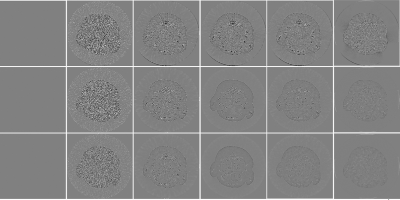
To further demonstrate the advantages of the SSCMF method, Fig. 7 shows the reconstructed difference images with respect to the references. Note that the reference images are reconstructed by the SART from noise-free projections. It can be seen from Fig. 7 that the reconstructed images utilizing the SART have the largest differences, followed by the TVM, TV+LR and TDL. In contrast, the difference images of SSCMF are smaller than those reconstructed using other competing algorithms, especially for the 1^th energy channel.

Fig. 7.

Same as Fig. 4 but the difference images with respect to references. The display window is [−0.2, 0.2] cm⁻¹.

To quantitatively evaluate the reconstructed image quality, the indexes of root mean square error (RMSE), peak signal-to-noise ratio (PSNR) [37], feature similarity (FSIM) [38] and structural similarity (SSIM) [39] are employed. Table 2 summarizes all the quantitative results which indicate that the SSCMF can obtain the smallest RMSEs for all channels, followed by the TDL and then TV+LR method which has slightly smaller RMSEs than the TVM. The SART has the largest RMSEs in all channels because of no prior knowledge. These conclusions are also confirmed with the indexes of PSNR, FSIM and SSIM.

Table 2.

Quantitative image quality evaluation results.

Index	Method	1st	2nd	3rd	4th	5th	6th	7th	8th
RMSE (10−2)	SART	11.88	8.50	6.85	6.23	6.07	6.35	6.00	5.72
	TVM	3.80	2.57	1.98	1.73	1.55	1.53	1.37	1.21
	TV+LR	3.69	2.34	1.73	1.40	1.22	1.34	1.14	0.98
	TDL	3.40	2.14	1.54	1.22	1.05	1.07	0.96	0.87
	SSCMF	2.68	1.62	1.18	1.03	0.88	0.88	0.78	0.73
PSNR	SART	18.50	21.40	23.28	24.11	24.33	23.94	24.44	24.86
	TVM	28.40	31.81	34.08	35.26	36.17	36.31	37.23	38.34
	TV+LR	28.67	32.60	35.25	37.09	38.29	37.43	38.86	40.13
	TDL	29.37	33.38	36.23	38.24	39.57	39.39	40.32	41.25
	SSCMF	31.44	35.83	38.53	39.74	41.10	41.14	42.11	42.76
SSIM	SART	0.9125	0.8838	0.8647	0.8273	0.7737	0.7251	0.6801	0.6291
	TVM	0.9901	0.9876	0.9835	0.9746	0.9595	0.9407	0.9220	0.8918
	TV+LR	0.9909	0.9877	0.9843	0.9759	0.9684	0.9583	0.9318	0.9152
	TDL	0.9909	0.9924	0.9943	0.9901	0.9896	0.9874	0.9724	0.9506
	SSCMF	0.9915	0.9956	0.9962	0.9949	0.9930	0.9911	0.9892	0.9865
FSIM	SART	0.8822	0.8345	0.8223	0.8037	0.7797	0.7567	0.7384	0.7177
	TVM	0.9780	0.9730	0.9713	0.9647	0.9497	0.9326	0.9246	0.9133
	TV+LR	0.9870	0.9836	0.9815	0.9722	0.9564	0.9365	0.9347	0.9238
	TDL	0.9822	0.9860	0.9876	0.9844	0.9811	0.9774	0.9597	0.9308
	SSCMF	0.9871	0.9909	0.9885	0.9855	0.9824	0.9794	0.9761	0.9711

b). Material Decomposition

The material decomposition of spectral CT images is a nonlinear ill-posed problem. Regarding the material decomposition methods, they mainly can be classified into two categories, i.e., projection-based and image-based methods. The projection-based methods model the nonlinear material decomposition problem and usually introduce regularization in the material-specific projection domain. Unfortunately, those methods are very sensitive to noise, and the decomposed images are highly affected by noise [40, 41]. Regarding the image-based methods, they first reconstruct all energy bin images independently using a set of different spectra and then obtain basis material images using a matrix inversion. Such an image-based method fails to characterize the real nonlinearity relationship between the polychromatic projections and the decomposed results. This may cause artifacts in the decomposed results [42].

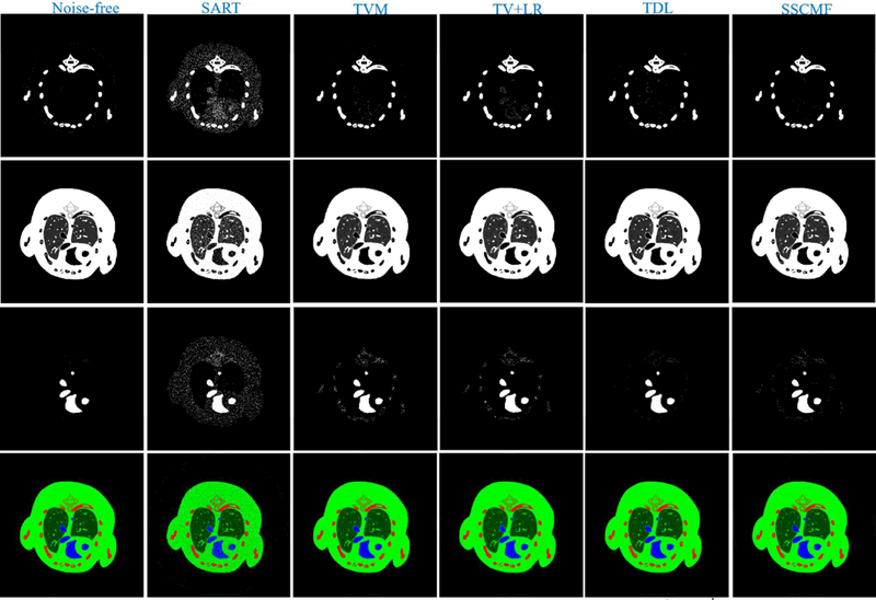
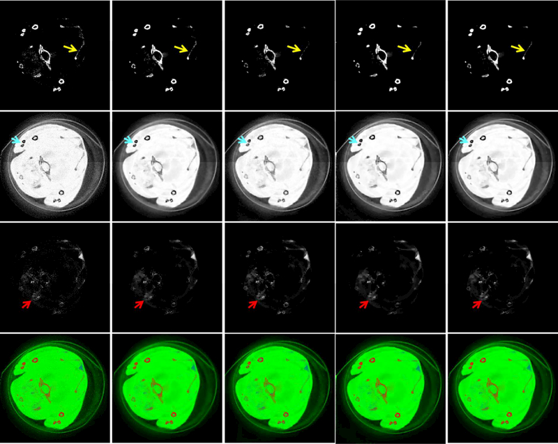
To validate the proposed SSCMF algorithm in terms of material decomposition, the reconstructed all channel images are decomposed into three basis materials (soft tissue ,bone and iodine contrast agent) utilizing an image-based material decomposition method [43]. Fig. 8 shows the proportions of the corresponding three basis materials and the individual merged color images. From the 1^st row of Fig. 8, it can be seen that more pixels of iodine contrast agents are easier to be wrongly classified into the bony regions by the SART, TVM, TV+LR and TDL methods than the SSCMF method. For the soft-tissue component decomposition (2^nd row), the SSCMF result provides more finer structures than those achieved by other competing algorithms. In terms of the iodine contrast agent decomposition component, the TDL and SSCMF methods have similar high accuracy. To quantitatively evaluate the material decomposition results, the RMSE, PSNR, SSIM and FSIM values of each basis material from all reconstruction methods are listed in Table 3.

Fig. 8.

Three basic materials decomposed from the reconstructed results in Fig.4. The 1st to 3rd rows represent bone, soft tissue and iodine. The 4th row images are color renderings, where red, green and blue represent bone, soft tissue and iodine, respectively. For the 1st to 3rd rows, the display windows are [0, 0.1], [0.2, 0.8] and [0, 0.5] cm⁻¹, respectively

Table 3.

Quantitative evaluation results of three decomposed basis materials.

Index	Method	Bone	Soft tissue	Iodine contrast agent
RMSE (10−2)	SART	1.27	6.77	4.96
	TVM	0.70	2.61	1.95
	TV+LR	0.85	2.67	1.87
	TDL	0.77	2.10	1.20
	SSCMF	0.50	1.90	1.19
PSNR	SART	37.92	23.39	26.08
	TVM	43.11	31.68	34.20
	TV+LR	41.40	31.47	34.59
	TDL	42.25	33.55	38.12
	SSCMF	46.06	34.44	38.50
SSIM	SART	0.9118	0.6176	0.7596
	TVM	0.9976	0.8923	0.9470
	TV+LR	0.9949	0.8654	0.9544
	TDL	0.9982	0.8424	0.9628
	SSCMF	0.9984	0.9687	0.9661
FSIM	SART	0.9899	0.8098	0.9084
	TVM	0.9985	0.9699	0.9578
	TV+LR	0.9981	0.9760	0.9581
	TDL	0.9986	0.9753	0.9604
	SSCMF	0.9988	0.9755	0.9604

c). Convergence Analysis

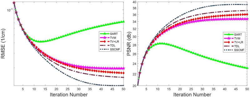
The SSCMF model contains the L₀-norm minimization of 4D groupwise coefficients, which is NP-hard and makes the convergence complicated. In this study, we only numerically analyze the convergence of the proposed method. Specifically, the averaged RMSE and PSNR vs. iteration number are given in Fig. 9. By comparison, the SSCMF algorithm can converge to an optimized solution quickly with a smaller RMSE or a higher PSNR. Because the spectral CT projection datasets contain severe noise, the RMSE values of SART decrease rapidly and then increase slowly. Fig. 9 indicates that the RMSEs can maintain subsequently stable after 40 iterations for all the reconstruction methods.

Fig. 9.

Convergence curves of averaged RMSE (a) and PSNR (b) vs. iteration number.

d). Parameters Selection

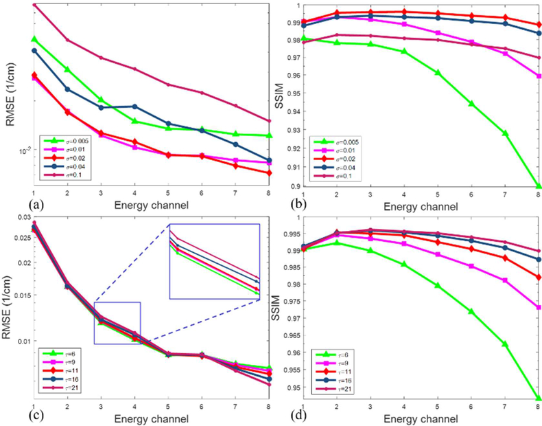
The parameters of SSCMF mainly include the estimated image noise level σ and the hard-threshold value τ. σ depends on the estimated noise at current iteration. That is to say, the higher the image noise levels is, the greater the σ value is. In this study, σ is set as a constant. Regarding the hard-threshold value, τ it is used to suppress noise by removing small coefficients in the 4D transform domain. A greater value of τ can enforce the anti-noising capability and lose more image details. Correspondingly, a smaller value of τ can decrease the anti-noising capability and keep more image details. Here, to investigate the performance of the SSCMF method with respect to different parameter settings, we quantitatively compare the RMSEs and SSIMs from all channels with respect a small σ (σ = 0.005) have large RMSEs and small SSIMs in all energy chanσ nels. A greater σ to one parameter, as shown in Fig. 10. Fig. 10 (a) and (b) show that the reconstructed images with (σ = 0.1) may lead to similar conclusions. This means an appropriate σ value can result in smalls RMSEs and large SSIMs. For this case, the optimal is around 0.016, which matches the noise level in the reconstructed image. From Fig. 10 (c) and (d), we can see that a smaller can result in a of SSIM, a greater τ might obtain better results. For this case, the optimal τ is around 11 and it was smaller RMSE in low energy channel and larger RMSE in high energy channels. In terms of the index set as 12.

Fig. 10.

Quantitative results of all energy channels with respect to different parameters.

e). Low-dose Reconstruction

To evaluate the performance of SSCMF in the case of low-dose reconstruction, the photon number of each x-ray path is reduced to 5×10³. The lower the photon number of each x-ray path is, the higher the Poisson noise in projection is. Fig. 11 shows the reconstructed images. From Fig. 11, it can be seen that the images reconstructed by the TVM, TV+LR and TDL methods loss some finer structures and details, especially in the high-energy channels. Compared with the TVM and TV+LR results, the images reconstructed by the SSCMF algorithm have clear image edges.

Fig. 11.

Same as Fig.4 but reconstructed with 5×10³ photons per x-ray path.

f). Contrast Agent Concentration Analysis

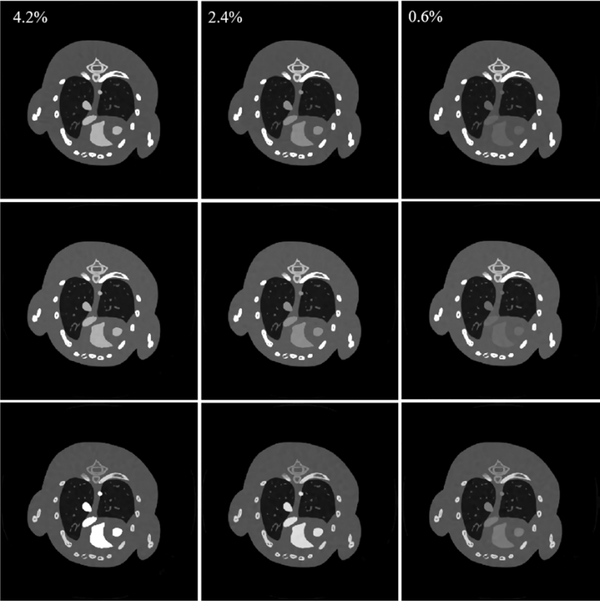
To validate the performance of the proposed SSCMF method for different concentrations of iodine, 0.6%, 2.4% and 4.2% iodine concentrations are injected into the mouse thorax phantom, respectively. Fig. 12 demonstrates the reconstructed results, and it can be seen that the proposed SSCMF has a good performance with the selected iodine contrast concentration. The higher the iodine concentration is, the larger the image contrast is. In clinical applications, it is appropriate to select the iodine contrast concentration so that the final material decomposition results can separate three basis materials.

Fig. 12.

Results reconstructed by the SSCMF method with different iodine concentrations. From 1^st to 3^rd columns, the iodine concentrations are 4.2%, 2.4% and 0.6%, respectively. The 1^st to 3^rd row images correspond to the 1^st, 4^th and 8^th channels, and their display windows are [0, 3], [0, 1.2] and [0, 0.8] cm⁻¹, respectively

g). Computational Cost Analysis

Regarding the computational costs of all the optimization algorithms, i.e., TVM, TV+LR, TDL and SSCMF methods, they can be divided into two major procedures: backprojection reconstruction and regularization constraint. The computational cost of multi-energy projection datasets reconstruction step mainly depends on the number of energy channels. The higher the number of energy channels is, the larger the time consumption is. Regarding the regularization term, different regularization constraints have different computational costs and they also depend on the parameter settings. For example, the computational cost of CMF depends on the tensor cube size, search tensor cube window size, the cube sliding step, etc. In general, the computational cost to update the regularization term is less than that is consumed by the back projection reconstruction. In this study, all the aforementioned methods are programmed by Matlab (2017b) with GPU techniques on a PC (8 CPUs @3.40GHz, 32.0GB RAM, Intel(R) HD Graphics 530). Here, the back projection reconstruction step consumes114.58 seconds in all algorithms. For the TV, TV+LR, TDL and CMF regularization terms, they cost 1.64, 0.52, 10.65, 38.23 seconds, respectively. The CMF regularization term requires more time than the TV and TV+LR regularizations because it is performed on overlapped small image tensor cubes. Because the number of TV iteration is 20 and it needs to operate on each channel image independently, the TV regularization needs more computational costs than the TV+LR method.

4.2. Preclinical Mouse Study

A mouse with injected gold nanoparticles (GNP) was scanned by a MARS micro spectral CT system. The system includes one x-ray source and one PCD. The distances from the x-ray source to the PCD and rotation axis are 255 mm and 158 mm, respectively. The PCD horizontally consists of 512 elements, and each element covers a length of 0.11 mm, resulting in an FOV with a radius of 9.21mm. 371 raw projections are collected in a full scan. A strategy of multiple scans is adopted, and 13 energy channel datasets are obtained. The projections for the central slice in fan-beam geometry Each reconstructed channel image is a matrix of 512×512, covering area of 18.41×18.41mm². are extracted and employed to verify the advantages of the SSCMF algorithm in practical applications.

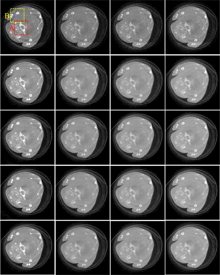
Fig. 13 shows the reconstructed results of four representative energy channels (1^st, 5^th, 9^th and 13^th). From the 1^st row of Fig. 13, it can be seen that the images reconstructed by the SART are corrupted by severe noises and lose some details. Although the reconstructed images using the TVM and TV+LR methods (2^nd and 3^rd rows in Fig. 13) contain less noise, the soft tissue structures are blurred to some degree, especially the obvious blocky effects in the TVM reconstruction. In contrast, the TDL and SSCMF methods achieve a great success in recovering finer structures as well as preserving image edges (see the 4^th and 5^th rows).

Fig. 13.

Reconstructed results of four representative energy-channels. From the 1^st to 4^th columns, the images are for different energy-channels (1^st, 5^th, 9^th and 13^th). From the 1^st to 4^th rows, the images are reconstructed using the SART, TVM, TV+LR and SSCMF methods, respectively. The display window for all the reconstructed images are [0, 0.8] cm⁻¹.

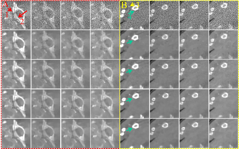
To further demonstrate the advantages of the SSCMF method, a bony ROI A and soft tissue ROI B are extracted and magnified as in Fig. 14. For the magnified bony ROI A, one can see that the image structures indicated by the red arrows “1” and “2” can hardly be distinguished in the images reconstructed by the SART, TVM and TV+LR methods. The image structure indicated by the red arrow “2” is slightly blurred in the images reconstructed by the TDL technique. However, the images reconstructed by the SSCMF have clearer edge features. As for the soft tissue ROI B, we can see that the images reconstructed by the SSCMF are smoother with more image details. The region marked with the arrow “3” indicates the unique merits of the TDL and SSCMF in recovering fine structures. The image edge structures indicated by arrow “4” is more clearer using the SSCMF than that obtained from the TDL method.

Fig. 14.

The magnified ROIs A and B in Fig.13.

Regarding the material decomposition, Fig. 15 shows three decomposed basic materials (tissue, bone and GNP) and color rendering images. For the bone material, the profile of SSCMF is clearer than those obtained from the SART, TVM, TV+LR and TDL methods. In addition, the SSCMF can also provide more accurate tissue decomposition results without blocky artifacts. In the rendered color images, the edges of the SSCMF method are more obvious than other competing algorithms.

Fig. 15.

Three decomposed basic materials of the Fig. 13. From the 1^st to 3^rd rows, the images are for bone, soft tissue and GNP, respectively. The 4^th row images are merged color images, where red, green and blue represent bone, soft tissue and GNP, respectively. For the 1^st to 3^rd rows, the display windows are [0.1, 0.5], [0, 1] and [0, 0.5] cm⁻¹, respectively.

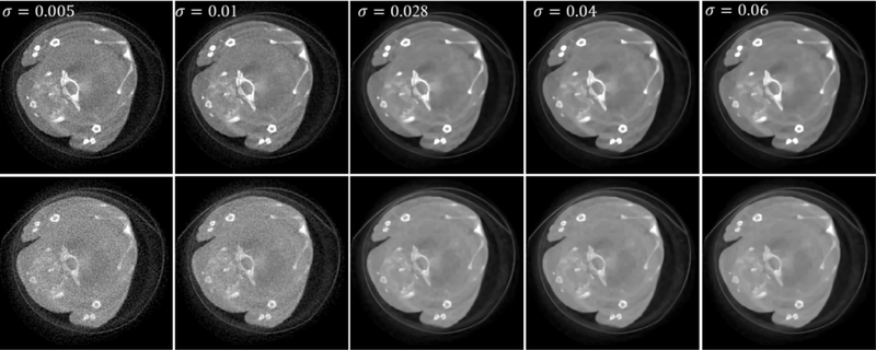
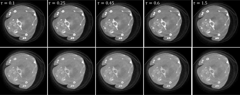
To further analyze the impacts of the parameters on the reconstructed image quality in practical series of different parameter settings. From Fig. 16, it can be seen that a small σ value (0.005 and 0.01) applications, Figs. 16 and 17 show the reconstructed mouse images using the SSCMF method with a can reduce the algorithm robustness and a greater σ value (0.028, 0.04 and 0.06) can smear finerτ structures and image edges. Regarding the selection of parameter , a similar conclusion can be made.

Fig. 16.

Reconstructed results with different σ. The 1^st and 2^nd rows represent different channels (1^st and 13^th). From the 1^st to 5^th columns, the images are reconstructed with different σ and a fixed τ = 0.35. The display window is [0, 0.8] cm⁻¹.

Fig. 17.

Same as Fig. 16 but with different τ and a fixed σ = 0.016.

5. Discussions and Conclusions

Although the SSCMF method reconstructs excellent results for the spectral CT, there are still some issues to be addressed. First, there are numerous parameters in the BM4D denoising procedure to be optimized for Eq. (25), including the tensor cube size, tensor cube searching window size, the number of tensor cubes, etc. In this work, we only empirically optimized the main parameters based on extensive experiments. However, the theoretical analysis of optimization for all parameters is still open. Second, different similarity measurements for cubes may generate different groups and further result in different reconstruction results. In this study, the sum of squared differences between two input tensor cubes is considered as the similarity measurement [22], which can be read as

$$d\left({\mathcal{Y}}_{j,r},{\mathcal{Y}}_{j,l}\right)=\frac{{\Vert {\mathcal{Y}}_{j,r}-{\mathcal{Y}}_{j,l}\Vert }_F^2}{L^3},$$

where L³ is a normalized factor. Of course, there are other methods to quantify such similarity, such as SVM-KNN [44], PCA basis [45], etc. In our future work, we will investigate the reconstructed results with respect to different similarity measurements. Third, because the BM4D denoising codes are only implemented on CPU, we will transplant this procedure to GPU to speedup the convergence. Fourth, we only employ a simple strategy to solve Eq. (16). In fact, there are many other available methods, such as split-bregman method [8], alternative direction minimization method (ADMM) [46], etc. Fifth, because a volumetric CT image has 3D similar structures, the proposed CMF regularization term can be directly applied for 3D volumetric CT reconstruction. Furthermore, a 4DCT image not only has similarity in 3D volumetric space but also has structural and intensity similarities among different time frames. Moreover, as for the cone-beam spectral CT reconstruction, it is necessary to extend the established CMF to 5D so that it can explore both the 3D volumetric structures and 1D spectral similarities.

In this study, the numbers of energy channel are 8 and 13 in numerical simulation and clinical experiment, respectively. In practice, the number of energy channel may be smaller. To evaluate the proposed method for the case with less channels, the aforementioned spectrum in numerical simulation is divided into four different energy channels: [16, 25) keV, [26, 33) keV, [34, 40) keV, [41, 50) keV. Fig. 18 shows all channel images reconstructed by using the SSCMF method. It can be observed that the SSCMF algorithm still perform well in reconstructing high quality images from less energy channels.

Fig. 18.

Reconstructed results from 4 energy channels. From left to right, the images are for 1–4 energy channels and their display windows are [0, 2] cm⁻¹, [0, 1.2] cm⁻¹, [0, 1.0] cm⁻¹ and [0, 0.6] cm⁻¹, respectively.

In summary, to take advantages of the similarity of nonlocal spatial-spectral cubes in spectral CT images, we first propose a CMF for BM4D procedure, and then it is introduced into the spectral CT reconstruction model as a new regularizer. By incorporating the CMF into basic spectral CT reconstruction model, the reconstructed image quality is dramatically improved. The advantages of the SSCMF method are twofold. First, it can explore both the nonlocal similarity of an image and structural similarity among different spectral channels by grouping similar spatial-spectral cubes. This makes it a great success for the SSCMF method to preserve image edges and recover finer structures. Second, performing collaborative filtering on the raw group and 1^st estimation can improve the algorithm robustness. Both numerical simulations and realistic preclinical mouse experiments confirm these merits of the proposed SSCMF method by comparing with the SART, TVM, TV+LR and TDL methods.