Statistical outbreak detection by joining medical records and pathogen similarity

Abstract

We present a statistical inference model for the detection and characterization of outbreaks of hospital associated infection. The approach combines patient exposures, determined from electronic medical records, and pathogen similarity, determined by whole-genome sequencing, to simultaneously identify probable outbreaks and their root-causes. We show how our model can be used to target isolates for whole-genome sequencing, improving outbreak detection and characterization even without comprehensive sequencing. Additionally, we demonstrate how to learn model parameters from reference data of known outbreaks. We demonstrate model performance using semi-synthetic experiments.

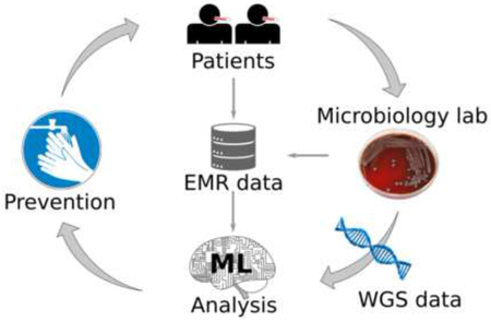
Graphical Abstract

1. Introduction

Hospital-associated infections (HAIs) are an unfortunate reality in the hospital setting. The Centers for Disease Control and Prevention estimated that 722,000 HAIs occurred in the U.S. acute care hospitals in 2011, resulting in 75,000 deaths [23]. Some HAIs represent hospital-associated transmission (HAT), in which bacteria or other pathogens are transmitted in the hospital. In addition, because of HAI case definitions, not all HAT is considered to be HAI.

Under the current standard of practice, investigation into potential instances of HAT are conducted in response to reports of suspicious infections by hospital staff or review of HAIs by infection prevention teams. Review of HAIs can identify circumstantial similarities among infection cases and exposures that may be indicative of HAT [12, 1]. This process may be iterative, working from an initial group of suspicious infections and adding or removing cases as evidence is accumulated. Evidence for common exposure is often found by reviewing electronic medical records (EMR), which can be labor intensive for complex hospital stays involving, for example, a patient being housed in different locations within the hospital or involving multiple medical procedures. High levels of genetic similarity across pathogens is often indicative of possible transmission, though whether such infections constitute HAT is contingent on the nature of their relationship. For example, transmission may have occurred at a common long-term care facility prior to arrival at the hospital. While understanding such instances may be clinically relevant they may not be considered HAT.

Due to falling costs and high discriminatory power, it is becoming feasible to use whole genome sequencing (WGS) as a basis for measuring genetic similarity of pathogens in clinical practice. A common measure of genetic similarity during outbreak investigations involving HAT is the single-nucleotide polymorphism (SNP) differences between bacterial isolates. Sequencing environmental or device isolates is commonly performed to adjudicate hypothesized root-cause exposures [24]. Upon identification of the root-cause, infection prevention teams can intervene to mitigate subsequent transmission and, ideally, similar outbreaks in the future. Interventions may include removing a contaminated device from clinical service, sanitizing contaminated hospital environments, educating healthcare personnel to improve infection prevention practice, or other suitable actions.

There is a need to improve HAT identification [1, 28] and root-cause analysis to reduce the risk of outbreaks going unnoticed and to reduce the time between launching an investigation and root-cause identification, thus allowing timely and effective interventions. We present a statistical framework for analysis of HAT that (i) comprehensively monitors patient exposures and clinical microbiology records to detect cases of HAT, (ii) probabilistically ranks potential root-causes, and (iii) suggests which patients’ isolates to submit for WGS to maximize performance on tasks (i) and (ii) under budgetary and resource constraints. We demonstrate the performance of our proposed approach using semi-synthetic data experiments. Our results suggest that the proposed approach to monitoring may be operationally effective at improving HAT detection and investigation in practical settings.

The remainder of the document is structured as follows. In Section 2 we review related work, Section 3 presents our model and methods for inference, Section 4 demonstrates the approach on semi-synthetic simulations constructed from known historical outbreaks. Finally, Section 5 concludes with some remarks on the strengths and weaknesses of the approach, issues to consider for deployment, and alternative strategies.

2. Related Work

The concept of ‘outbreak’ can mean either an unexpected increase in the number of disease cases, or the introduction of a pathogen strain into a particular environment [12]. Here we use the term, as does much of the related literature, in the latter sense. The related literature largely breaks down along lines of outbreak detection and outbreak characterization. Outbreak detection methods often use primarily count based statistics to identify groups of patients for whom the number of infections is unusually large [10]. Outbreak characterization methods primarily focus on reconstructing the transmission tree for a given outbreak. Little work is apparent at the intersection of these two viewpoints, in particular when the number of cases per incident is very small.

2.1. Bio-surveillance

de Bruin et al. [7] review 27 early electronic HAI surveillance systems for effectiveness. The authors focus on how data sources leveraged by these systems correlate with reported performance. It was noted that increased use of EMR was correlated with a shift toward increased sensitivity and decreased specificity. Hota et al. [17] translated manual chart review processes for bloodstream infection into an automated algorithm. The authors identified heterogeneous nomenclatures and a lack of standardized data as a major challenge. Other studies have demonstrated that electronic surveillance out performs manual efforts while reducing overall effort [6, 31]. Yet, it has been pointed out that automated systems may miss cases in which critical evidence, such as remarks in physician’s narratives, are not included in the electronic analyses [31].

Deng et al. [8] reviewed the use of WGS in bio-surveillance in the food industry. The authors point toward cases in which the combination of WGS and epidemiological data were able to improve precision of investigative efforts; ruling out potential causes that looked plausible based on epidemiological data alone. Hill et al. [15] used simulation to study the benefit of combining WGS with epidemiological data, in the form of tracking individual food units. The authors stressed the importance that the epidemiological data be relevant; capturing important system dynamics.

Stachel et al. [29] evaluated WHONET [32] in combination with SaTScan [27] (WHONET-SaTScan) as a tool for combining EMR and microbiological culture data for outbreak detection. The approach is to find spatio-temporal regions in which the number of observed infections is significantly higher than expectation, based on comparable baselines derived from the outside of the region of interest. The analysis considered cultures collected not less than 3 days after admission and analyzed hospital, unit, and service lines as spatial dimensions. Identified groups of patients were escalated for investigation if they met 3 of 6 criteria that included common exposure and pathogens with similar antibiotic susceptibility profiles.

Grad and Lipsitch [12] discuss in detail many of the issues and opportunities at the heart of outbreak detection and characterization from the perspective of public health. The need to be robust is a common theme across issues of sampling, genetic measurements, data and analysis development, and inference. Often many sources of information may be incomplete, inference may be incorrect or uncertain, and there may be privacy and legal concerns.

2.2. Transmission tree reconstruction

Largely motivated by falling costs for WGS, recently there has been significant interest in using high precision genomic techniques in combination with epidemiological data to characterize outbreaks of infectious disease. These efforts have largely focused on reconstructing the transmission tree from observed data. Generally, these methods do not focus on root-cause analysis. Unless health-care workers, devices, linens, and other environmental factors are sampled, they will not be included in the reconstructed transmission tree and any outbreak stemming from such potential causes will not be correctly explained by the transmission tree alone. A notable exception is [9] which accounts for partially observed outbreaks with unsampled “hosts.” However, to the extent that patient-to-patient transmission can be reliably identified, some potential root-causes may be ruled out. We view this body of literature as germane to outbreak detection and characterization, but a full review of this literature is beyond the scope of this paper. For relevant reviews, we refer the reader to Ray et al. [26] and Hatherell et al. [14].

Cottam et al. [4] and Cottam et al. [5] have been pointed to as seminal papers in the combination of molecular and epidemiological data for outbreak characterization [26, 21]. Cottam et al. [5] developed a probability model describing the likelihood of farm-to-farm virus transmission that incorporated known infection timings. The authors demonstrate that the addition of the epidemiological data significantly increases the power of inference over genetic evidence alone. Jombart et al. [19] use a maximum weight spanning tree approach constrained to respect time ordering of isolates. Lapidus and Carrat [22] developed a probabilistic model based on contacts between infected subjects and chronology of disease symptoms to infer likely transmission trees. More recently, many authors have employed Bayesian modeling and the accompanying Markov Chain Monte Carlo (MCMC) sampling methods to perform inference over transmission trees [35, 13, 20, 25]. Such models usually include mathematical terms that describe the likelihood of the infected population and measured pathogen similarities under a supposed transmission tree. MCMC sampling is then conducted to make inferences (usually on the transmission tree), such as finding the most likely tree.

Worby et al. [34] introduced a geometric-Poisson model for inferring the likelihood of SNP distance between pairs of isolates in the same outbreak based on the time of lineage divergence, sampling times, and expected time of coalescence. The authors demonstrate that probabilistic reasoning using the model outperformed previous graph based [19] and Bayesian [20] approaches at identifying cases of direct transmission. The authors note that the method performs best when there is a high mutation rate. However, other studies have suggested that outbreaks, in fact, tend to have low genetic diversity [19, 3].

Worby et al. [35] propose a full Bayesian model for computing the posterior probability of transmission routes. The model relaxes several assumptions common in prior work including known infection times, fully connected transmission trees, and presumed irrelevance of the uninfected population. Similar to [34], it assumes either a Poisson or geometric distribution on SNP distances. The model further assumes homogeneous mixing of patients within a hospital, modeling the transmission likelihood using an exponential distribution. The authors explore the improvements that can be gained by considering shared genetic variants when computing genetic similarity.

Frequent criticisms of the above approaches include that they require densely sampled genetic data (most/all of the constituent individuals in an outbreak), either require a model of within-host diversity (which may not be known) or fail to account for within-host diversity, and ignore individuals who avoided infection [12, 35, 26, 14]. Didelot et al. [9] relaxes the need for dense genetic sampling, improving the utility of transmission tree inference for ongoing outbreak investigation.

3. Methods

As noted above, a number of researchers have observed that WGS based measures of pathogen similarity cannot resolve all of the uncertainty in the transmission tree. To use WGS most advantageously, proper models of within- host population dynamics, within-environment population dynamics, and transmission bottleneck sizes, are required. Further, the genetic similarity of distinct lineages of a given pathogen are a function of the local environment. Unfortunately, the necessary information to account for these factors may not be wholly available for most pathogens and/or environments a priori. Furthermore, in this application, important portions of the available epidemiological data can be expected to be co-opted from existing data streams designed to serve other purposes (e.g. billing). Therefore, the derived epidemiological data may be coarse, incomplete, or otherwise suboptimal for HAT detection and root-cause analysis. Finally, recent studies have pointed to high degrees of uncertainty in resolving transmission trees from genetic data, due to low within-outbreak genetic diversity [34, 3].

We therefore attempt to find a middle ground between exploiting the available genetic and epidemiological data, and being robust to those issues. We accomplish this in two ways. First, we do not try to infer the complete transmission tree. Since we are primarily concerned in HAT detection and secondarily in root-cause identification, the underlying transmission tree is only of tertiary interest. Second, we use machine learning approaches to learn, from historical examples, the within-outbreak transmission probabilities conditioned on the observed epidemiological data. This allows the model to incorporate and contextualize the epidemiological information without being overly constrained by it.

For the semi-synthetic experiments performed here, epidemiological data include admission, discharge, and isolate collection dates, room and unit occupancy, as well as the date and type of each procedure undergone by each patient. We refer to these pieces of information as EMR data. Genetic data include pathogen species and antibiotic resistance profiles. Since species identification and measurement of antibiotic resistances are routine in most hospitals, we include these elements in our reference to EMR data. Our experiments consider exposures to 245 of the most common procedures and procedure groups. We refer to pairwise SNP distances as WGS data. In the simulation experiments presented here, the EMR data used are real-world and the WGS data are generated synthetically.

3.1. Direct/Indirect Transmission Outbreak (DITO) model

We propose a simple inference model for outbreak detection and characterization. The model considers only the top of the transmission tree, i.e. those patients infected by the root-cause, leaving the remainder of the tree undefined. We show how the structure of this model allows analytic maximization or marginalization over the set of patients infected by the root-cause. This approach results in a flexible probabilistic model with which the presence of an outbreak, as well as its constituent patients and root-cause can be inferred simultaneously.

We begin by introducing some notation. Let $\mathcal{I}$ denote a set of infected patients, for example: all patients with a positive culture for a common species of bacteria within a fixed window of time (analysis window). Let ${\mathcal{O}}_r\subseteq \mathcal{I}$ be a decorated¹ set of patients who are part of an outbreak with root-cause r. Here, we presume a single outbreak, though our methods can be extended to multiple concurrent outbreaks. Let ${\epsilon }_r$ be the set of patients exposed to the root-cause, which infects patients upon exposure with probability θ. The set ${\epsilon }_r$ includes non-infected patients as well as infected patients. Infected patients are only included in ${\epsilon }_r$ if they were exposed to the root-cause before their positive culture (time of isolate collection). Then, the set $a\subseteq {\mathcal{O}}_r\cap {\epsilon }_r$ identifies the patients in the outbreak who were infected by the root-cause. For each patient $i\in \mathcal{I}$, we denote the probability that patient i was infected by a not-HAT cause as η_i. We denote the probability that patient $i\in {\mathcal{O}}_r$ was infected by intermediate transmission (indirect) as γ_i.

The probability η_i can be an arbitrary function of patient i’s characteristics (e.g. age, gender, medical history, and/or co-morbidities) and is assumed to not depend on a, or θ. The probability γ_i is also assumed to not depend on a or θ, but can otherwise be a function of the specific outbreak instance ${\mathcal{O}}_r$. This might include isolate collection time, the size of the outbreak, co-residence with previously infected within-outbreak patients, and/or patient specific characteristics. For the purposes of our experiments, we take η_i and γ_i to be constants, but treat them as general functions in the following presentation. In Section 3.2 we demonstrate how these functions can be determined from historical outbreak data using machine learning.

We take $\mathcal{S}$ to denote some notion of infection similarities. These similarities may be derived from WGS (e.g. SNP distance), or antibiotic susceptibility patterns, or some combination of the two. Following [35], we treat pairwise similarities as mutually independent, conditioned on whether the infections are of common origin. Let $S_{i,j}^{+}$ be the probability of the observed similarity between the infections of patients i and j conditioned on $i,j\in {\mathcal{O}}_r$. Let $S_{i,j}^{-}$ be the probability of the observed similarity otherwise (i.e. i and j not both in ${\mathcal{O}}_r$). S⁺ and S⁻ are assumed to not depend on a or θ. Here, we treat them as fixed (i.e. independent of ${\mathcal{O}}_r$) symmetric matrices with $S_{i,i}^{+}=S_{i,i}^{-}=1$. Under these assumptions, the probability of $\mathcal{S}$ is modeled as

$$\mathbb{P}(\mathcal{S}\mid \mathcal{I},{\mathcal{O}}_r)=\prod _{i,j\in \mathcal{I},i<j}[S_{i,j}^{+}{\mathrm{𝟙}}_{\{i,j\in {\mathcal{O}}_r\}}+S_{i,j}^{-}(1-{\mathrm{𝟙}}_{\{i,j\in {\mathcal{O}}_r\}})],$$ (1)

where ${\mathrm{𝟙}}_{\{\cdot \}}$ is the indicator function.

Under this framework, there are three possible explanations for each patient infection; non-HAT ($i\in \mathcal{I}\setminus {\mathcal{O}}_r$), infected through the particular root-cause (i ∈ a), or infected by intermediate transmission within the outbreak ($i\in {\mathcal{O}}_r\setminus a$). The probability of observing the infected patient population given these explanations is given by

$$\mathbb{P}(\mathcal{I}\mid {\mathcal{O}}_r,a,\theta )={\theta }^{\mid a\mid }(1-\theta {)}^{\mid {\epsilon }_r\setminus a\mid }\prod _{i\in {\mathcal{O}}_r\setminus a}{\gamma }_i\prod _{i\in \mathcal{I}\setminus {\mathcal{O}}_r}{\eta }_i.$$ (2)

Combining (1) and (2), the probability of the observed data and likelihood ratio are given by

$$\begin{gathered} \mathbb{P}(\mathcal{S},\mathcal{I}\mid {\mathcal{O}}_r,a,\theta )=\mathbb{P}(\mathcal{S}\mid \mathcal{I},{\mathcal{O}}_r,a,\theta )\mathbb{P}(\mathcal{I}\mid {\mathcal{O}}_r,a,\theta ) \\ =\mathbb{P}(\mathcal{S}\mid \mathcal{I},{\mathcal{O}}_r)\mathbb{P}(\mathcal{I}\mid {\mathcal{O}}_r,a,\theta ) \\ \frac{\mathbb{P}(\mathcal{S},\mathcal{I}\mid {\mathcal{O}}_r,a,\theta )}{\mathbb{P}(\mathcal{S},\mathcal{I}\mid {\mathcal{O}}_r=\varnothing .)}={\theta }^{\mid a\mid }(1-\theta {)}^{\mid {\epsilon }_r\setminus a\mid }\prod _{i\in a}\frac{1}{{\gamma }_i}\prod _{i\in {\mathcal{O}}_r}\frac{{\gamma }_i}{{\eta }_i}\prod _{i,j\in {\mathcal{O}}_r,i<j}\frac{S_{i,j}^{+}}{S_{i,j}^{-}}. \end{gathered}$$ (3)

Equation (3) represents the likelihood ratio of the observed data under an outbreak to the null hypothesis; ${\mathcal{O}}_r=\varnothing$. where $\mathbb{P}(\mathcal{S},\mathcal{I}\mid {\mathcal{O}}_r=\varnothing .)={\prod }_{i,j\in \mathcal{I}}{S}_{i,j}^{-}{\prod }_{i\in \mathcal{I}}{\eta }_i$. Considering this ratio cancels out terms corresponding to non-outbreak patients. In the presence of an outbreak we expect to find an ${\mathcal{O}}_r$ and a that cause (3) to give a high value. Whereas in the absence of an outbreak we expect that one cannot find both a set of patients with high infection similarities ${}^{S_{i,j}^{+}}∕_{S_{i,j}^{-}}$. and a root-cause r with few negative exposures $\mid {\epsilon }_r\setminus a\mid$ and high coincidence ∣a∣. We therefore infer the presence, cause, and constituents of an outbreak by maximizing (3). To perform maximum likelihood inference, we will need to maximize (3) over ${\mathcal{O}}_r$, a, and θ. We will maximize over a and θ analytically and then turn to numerical methods to complete the inference. Additionally, in Section 3.3 we require the probability of an outbreak ${\mathcal{O}}_r$ to optimize a decision reward function. This too can be computed analytically by assuming e.g. uniform priors and marginalizing over a and θ. It is toward these two tasks that we turn our attention now.

Maximizing over a and θ.

The θ terms in (3) take their maximal value at ${\theta }^{\star }={}^{\mid a\mid }∕_{\mid {\epsilon }_r\mid }$. For any fixed ∣a∣, ${\prod }_{i\in a}{}^1∕_{{\gamma }_i}$ can be maximized by taking the first ∣a∣ patients sorted by γ_i in ascending order. Therefore (3) can be maximized in a and θ in $\mathcal{O}(\mid {\mathcal{O}}_r\mid \log \mid {\mathcal{O}}_r\mid )$ time, assuming the γ_i can be computed efficiently, by first sorting the patients in ${\mathcal{O}}_r$ and then iterating over values of ∣a∣ from 1 to $\mid {\mathcal{O}}_r\cap {\epsilon }_r\mid$. Note that a = ∅ is a degenerate solution, and is disallowed. Supposing the patients are sorted by γ_i, let a* be the value of ∣a∣ that maximizes (3). Then, the contribution due to the choice of route r is

$$\prod _{i=1}^{a^{\star }}\frac{1}{{\gamma }_i}{\left[\frac{a^{\star }}{\mid {\epsilon }_r\mid }\right]}^{a^{\star }}{\left[\frac{\mid {\epsilon }_r\mid -a^{\star }}{\mid {\epsilon }_r\mid }\right]}^{(\mid {\epsilon }_r\mid -a^{\star })}$$ (4)

and (3) takes the value P*:

$$P^{\star }({\mathcal{O}}_r)=\prod _{i\in {\mathcal{O}}_r}\frac{{\gamma }_i}{{\eta }_i}\prod _{i,j\in {\mathcal{O}}_r,i<j}\frac{S_{i,j}^{+}}{S_{i,j}^{-}}\prod _{i=1}^{a^{\star }}\frac{1}{{\gamma }_i}{\left[\frac{a^{\star }}{\mid {\epsilon }_r\mid }\right]}^{a^{\star }}{\left[\frac{\mid {\epsilon }_r\mid -a^{\star }}{\mid {\epsilon }_r\mid }\right]}^{(\mid {\epsilon }_r\mid -a^{\star })}.$$ (5)

Marginalizing over a and θ.

Integrating over θ gives the Beta function. Since ∣a∣ and $\mid {\epsilon }_r\setminus a\mid$ are integers, we have ${\int }_0^1{\theta }^{\mid a\mid }(1-\theta {)}^{\mid {\epsilon }_r\setminus a\mid }d\theta ={\left[(\mid {\epsilon }_r\mid +1)\left(\begin{array}{c}\hfill \mid {\epsilon }_r\mid \hfill \\ \hfill \mid a\mid \hfill \end{array}\right)\right]}^{-1}$. It remains to sum over values of a. We first consider sets of fixed cardinality. Let ${\xi }_m={\sum }_{a,\mid a\mid =m}{\prod }_{i\in a}{}^1∕_{{\gamma }_i}$, then

$$\frac{\mathbb{P}(\mathcal{S},\mathcal{I}\mid {\mathcal{O}}_r)}{\mathbb{P}(\mathcal{S},\mathcal{I}\mid {\mathcal{O}}_r=\varnothing .)}=\frac{1}{(\mid {\epsilon }_r\mid +1)}\prod _{i\in {\mathcal{O}}_r}\frac{{\gamma }_i}{{\eta }_i}\prod _{i,j\in {\mathcal{O}}_r,i<j}\frac{S_{i,j}^{+}}{S_{i,j}^{-}}\sum _{m=1}^{\mid {\mathcal{O}}_r\cap {\epsilon }_r\mid }{\xi }_m{\left(\begin{array}{c}\hfill \mid {\epsilon }_r\mid \hfill \\ \hfill m\hfill \end{array}\right)}^{-1}.$$ (6)

As it happens, the vector ξ can be computed efficiently by adapting a discrete Fourier transform based approach proposed by [16]. In brief, we define a vector x, with elements $x_l=\frac{1}{\mid {\mathcal{O}}_r\cap {\epsilon }_r\mid +1}{\prod }_{j=1}^{\mid {\mathcal{O}}_r\cap {\epsilon }_r\mid }1+\frac{1}{{\gamma }_j}\text{exp}\left(\frac{2\pi l\sqrt{-1}}{\mid {\mathcal{O}}_r\cap {\epsilon }_r\mid +1}\right)$, $l=0,\dots ,\mid {\mathcal{O}}_r\cap {\epsilon }_r\mid$. Then, ξ is given by the discrete Fourier transform of x. In this way, ${\sum }_{m=1}^{\mid {\mathcal{O}}_r\cap {\epsilon }_r\mid }{\xi }_m{\left(\begin{array}{c}\hfill \mid {\epsilon }_r\mid \hfill \\ \hfill m\hfill \end{array}\right)}^{-1}$ can be computed in $\mathcal{O}(\mid {\mathcal{O}}_r\cap {\epsilon }_r{\mid }^2)$ time. Again, a = ∅ is a degenerate case, and so the summation begins at m = 1.

3.2. Learning

Here, we demonstrate how the component probability functions of our model can be learned from historical data to better adapt the method to the local operating environment. There are four functions that need to be learned: ${}^{S_{i,j}^{+}}∕_{S_{i,j}^{-}}$ based on antibiotic resistance profiles, ${}^{S_{i,j}^{+}}∕_{S_{i,j}^{-}}$ based on SNP distance, η_i, and γ_i.

In our empirical data, not all bacterial isolates are tested for resistances to all antibiotics, moreover resistance information is often missing. Additionally, the number of known HAT outbreaks is small. In this situation, it is prudent to use a simple model that treats missing values as uninformative, such as a simple naïve Bayes model. For a given pair of bacterial isolates and antibiotic indexed by k, let c_k ∈ {−1, 0, 1} indicate whether the pair are both susceptible (c_k = −1), both resistant (c_k = 1), or one is susceptible while the other resistant (c_k = 0). The probability of c_k given that the pair of patients were part of the same outbreak $\mathbb{P}(c_k\mid y=1)$ (y denotes whether the pair is part of the same outbreak) can be estimated from historical outbreaks data. Similarly, the probability given that the pair of patients were not part of the same outbreak $\mathbb{P}(c_k\mid y=0)$ can be estimated by randomly sampling pairs. If outbreaks are rare, most such randomly assembled pairs will not be part of the same outbreak. We use Laplace smoothing to estimate the probabilities. Finally, we calibrate the estimated likelihood ratio using a logistic function. Specifically, this means we define $z_{i,j}=\text{ln}\left({\prod }_k\frac{\mathbb{P}(c_k\mid y=1)}{\mathbb{P}(c_k\mid y=0)}\right)$, then fit a logistic regression model to labeled pairs and take

$$\text{ln}\frac{S_{i,j}^{+}}{S_{i,j}^{-}}={\alpha }_2{z}_{i,j}+{\alpha }_1-\text{ln}({}^p∕_{1-p}),$$ (7)

where α are the logistic regression coefficients and p is the proportion of positive pairs in the training data. Equation (7) follows from ${}^{\mathbb{P}(x\mid y=1)}∕_{\mathbb{P}(x\mid y=0)}={}^{\mathbb{P}(y=1\mid x)\mathbb{P}(y=0)}∕_{\mathbb{P}(y=0\mid x)\mathbb{P}(y=1)}$, and we take $\mathbb{P}(y=1\mid z_{i,j})=[1+\text{exp}(-{\alpha }_2{z}_{i,j}-{\alpha }_1){]}^{-1}$ where y = 1 indicates within-outbreak and y = 0 otherwise.

To compute ${}^{S_{i,j}^{+}}∕_{S_{i,j}^{-}}$ using SNP distance, we can take exactly the same approach, except we exchange z_i,j in (7) for the SNP distance. This approach is directly related to the importation structure model proposed by [35] as a generative-discriminative pair; the importation model being the generative model. Both methods result in linear log-likelihood ratios.

Under the assumption that infections are common, but outbreaks are rare, one could use the probability of developing an infection as proxy ground truth to fit η_i. However, labels used for its estimation ought to be in good supply. One could fit any calibrated classification model to such proxy. Here we take η_i to be a constant, as thus take its value to be the mean proportion of patients who are infected.

The strategy we use to learn γ_i is to select its parameter values in such a way as to best differentiate the true root-cause from alternatives. For a fixed set of outbreak patients, only the θ and ${}^1∕_{{\gamma }_i}$ terms depend on the choice of route. Using historical outbreak data, we create a route score for each candidate route r, normalizing by outbreak-size, as

$$\underset{a\subseteq {\mathcal{O}}_r,\theta }{\max }\frac{1}{\mid {\mathcal{O}}_r\mid }\text{ln}\left({\theta }^{\mid a\mid }(1-\theta {)}^{\mid {\epsilon }_r\setminus a\mid }\prod _{i\in a}\frac{1}{{\gamma }_i}\right)=-\sum _{i=1}^{a_r^{\star }}\frac{\text{ln}{\gamma }_i}{\mid {\mathcal{O}}_r\mid }+\frac{C_r}{\mid {\mathcal{O}}_r\mid },$$ (8)

where $C_r=a_r^{\star }\text{ln}({}^{a_r^{\star }}∕{}_{\mid {\epsilon }_r\mid })+(\mid {\epsilon }_r\mid -a_r^{\star })\text{ln}{(}^{(\mid {\epsilon }_r\mid -a_r^{\star })}∕\mid {\epsilon }_r\mid )$ is a constant in the parameters of γ_i. The patients in ${\mathcal{O}}_r$ are taken to be the true (or known) outbreak population, regardless of the value of r. The parameter values of γ_i can then be learned using appropriate loss function (e.g. logistic loss) and optimization techniques. Dividing by $\mid {\mathcal{O}}_r\mid$ is a heuristic to make distinct outbreaks comparable for the purposes of learning. Here, we take γ_i to be constant, and so using logistic loss reduces to fitting a logistic regression model with a two column design matrix $X_{r,}.=\left[\frac{C_r}{\mid {\mathcal{O}}_r\mid },\frac{-a_r^{\star }}{\mid {\mathcal{O}}_r\mid }\right]$. That is, let $\mathbb{P}(y_r=1;\alpha )=[1+\text{exp}(\frac{a_r^{\star }}{\mid {\mathcal{O}}_r\mid }{\alpha }_1-\frac{C_r}{\mid {\mathcal{O}}_r\mid }{\alpha }_0){]}^{-1}$ and take ${\gamma }_i=\text{exp}({}^{{\alpha }_1}∕_{{\alpha }_0})$.

3.3. Inference

WGS recommendations..

We assume some information on strain similarity is available routinely. For example, antibiotic resistance profiles are routinely available in the experiments presented here. It is expected however, that WGS can provide measures of similarity (e.g. SNP distance) that are more precise, by which we mean better able to discriminate within-outbreak pairs from unrelated pairs. The availability of precise comparisons improves the quality of inference both in detection and characterization. We now demonstrate how our model can be used to give recommendations regarding which isolates ought to be selected for WGS given a fixed budget. We define a reward function $\mathbb{R}(d,{\mathcal{O}}_r)$ which measures the reward one would receive if a set of patients d was selected, given ${\mathcal{O}}_r$ is the true outbreak. One choice of reward measure might be the estimated increase in detection performance. Here we take $\mathbb{R}(d,{\mathcal{O}}_r)=\max \{1-{\left[\frac{2}{3}\mid d\cap {\mathcal{O}}_r\mid +\frac{1}{3}\right]}^{-1},0\}$ which serves to illustrate the approach. A reward function of this form saturates as more is learned about the outbreak mimicking an expected diminishing returns in the information gained about the root-cause. This encodes an exploitation versus exploration trade-off in a thusly established search strategy. Finally, we recommend $d^{\star }={\text{argmax}}_d{\mathbb{E}}_{{\mathcal{O}}_r}[\mathbb{R}(d,{\mathcal{O}}_r)]$ under the constraint that ∣d∣ ≤ K, where K is the budget (measured in number of WGS samples). To estimate the expected value we use (6) to perform importance sampling, described in Appendix B.

Maximum likelihood..

We use the above model to solve two inference problems. The first is to detect and characterize outbreaks, the second is to recommend isolates for whole-genome sequencing (not necessarily executed in that order). For detection and characterization we use a maximum likelihood approach, which means we must find the set of patients and route ${\mathcal{O}}_r$ that maximize (5). The pairwise similarity terms introduce a bilinear term with binary constraints in the logarithm of (5). Optimizing bilinear forms with binary constraints is known to be NP-complete [11]. The remaining terms are convex in a* when γ_i is constant. The result is that (5) is difficult to maximize.

We propose two remedial approaches. For both methods, we consider a set of patients and then maximize over routes by brute force as follows. If γ_i does not depend on r, then γ_i can be computed and patients sorted once for the set. Maximizing over r requires computing (4), which involves a set intersection to get ${\mathcal{O}}_r\cap {\epsilon }_r$ and a linear scan to find a*.

The first approach is a heuristic optimization strategy. For each choice of likelihood cutoff τ, we collect the sets of patients who are jointly connected by pairs where ${}^{S_{i,j}^{+}}∕_{S_{i,J}^{-}}>\tau$. Each such connected component is a candidate outbreak patient set. We sweep over all values of τ and then take the set of patients that yields max_r $P^{\star }({\mathcal{O}}_r)$. Finally, a rank of routes is produced by fixing the patient set and ordering the routes according to $P^{\star }({\mathcal{O}}_r)$. The second approach for optimizing over the patient set is to use cross-entropy optimization [2]. This is a simple general purpose stochastic strategy that has been shown to perform effectively, even on NP-complete problems [2]. In brief, outbreak patient sets are drawn by sampling patients without replacement. The proposal distribution is a mixture (in our experiments, we use 5 components) of patient-probability vectors. The top 25% of samples, ranked by max_r $P^{\star }({\mathcal{O}}_r)$ are then used to update the proposal distribution until convergence. We perform cross-entropy optimization using the complete infected patient population $\mathcal{I}$, and again for each cluster obtained by performing spectral clustering on the $\mathcal{I}$ using the ${}^{S_{i,j}^{+}}∕_{S_{i,j}^{-}}$ as the adjacency matrix (obtaining 15 clusters). We take the highest value over all clusters. This addendum is a simple heuristic strategy to focus additional effort on promising portions of the solution space.

We refer to the method of optimizing $P^{\star }({\mathcal{O}}_r)$ using cross-entropy optimization as ‘DITO^c,’ since it uses comprehensive WGS. The heuristic connected-component method is referred to as ‘${\mathbf{DITO}}_{\mathbf{H}}^{\mathbf{c}}$’. Optimizing $P^{\star }({\mathcal{O}}_r)$ using only antibiotic resistance based similarities (i.e. no WGS) is referred to as ‘DITO⁰.’ Recommending 10 isolates for WGS prior to inference by means of $d^{\star }={\text{argmax}}_d{\mathbb{E}}_{{\mathcal{O}}_r}[\mathbb{R}(d,{\mathcal{O}}_r)]$ is referred to as ‘DITO¹⁰.’

3.3.1. Baseline methods

We introduce four baseline methods to quantify the benefits of using the EMR data together with the WGS data. As our point of departure, recall that the DITO model uses WGS and/or similar data such as antibiotic susceptibilities to quantify the likelihood of a common origin through the $S_{i,j}^{+}∕S_{i,J}^{-}$ terms, and EMR data to determine exposure and approximate time of infection used to infer the sets of patients a and ${\mathcal{E}}_r$. The first baseline method uses no genetic data; we set $S_{i,j}^{+}∕S_{i,J}^{-}=1$, we call this ‘ExpR’ since it considers only exposures. The second method uses no EMR; we optimize ${\prod }_{i\in {\mathcal{O}}_r}\frac{{\gamma }_i}{{\eta }_i}{\prod }_{i,j\in {\mathcal{O}}_r,i<j}\frac{S_{i,j}^{+}}{S_{i,j}^{-}}$ instead of (5), which is accomplished using either cross-entropy optimization or the above heuristic. We call these ‘SIM’ when using cross-entropy optimization and ‘SIM_H’ when using the heuristic optimization. Finally, to demonstrate the performance of a pipeline inference strategy we rank routes by (4) using the outbreak patient population inferred by SIM, which we refer to as ‘SIM+(4)’.

Finally, we use CODA [18]; a CUSUM control charting method for detecting unexpected increases in a count of events, popular in bio-surveillance applications. Let C_t be the number of events in a fixed-width sliding window ending at time t. Here we take C_t to correspond to the number of pairs of patients with pairwise SNP distance less than a cutoff τ in a 7-day window. Let μ_t and σ_t be the mean and standard deviation for event counts at ‘similar’ times, learned from historical data. Here we take μ_t and σ_t to correspond to the mean and standard deviation of C_t in the same month of the previous 2 years. Then the control charting score CODA_t is computed as

$${\text{CODA}}_t=\max \left\{{\text{CODA}}_{t-1}+\frac{1}{{\sigma }_t}(C_t-{\mu }_t-{\sigma }_t),0\right\},$$ (9)

with CODA₀ = 0. An outbreak alert is generated if CODA_t rises above a decision threshold. The SNP cutoff τ can be chosen by maximizing Area Under Receiver Operating Characteristic (AUC) on historical outbreaks. The optimal cutoff turns out to be 0 for our simulations. We refer to ‘Coda₀’ as the CODA algorithm run on count of pairwise SNP distances equal to 0, ‘Coda_∞’ as the CODA algorithm run on count of pairs, and ‘Coda^#’ as the CODA algorithm run on count of patients. The later two do not use any WGS or EMR data apart from the count of infected patients.

3.4. Simulation environment

3.4.1. Data

The empirical data consist of all bedded patients at the University of Pittsburgh Medical Center (UPMC) Presbyterian Hospital, Pittsburgh, Pennsylvania between 2012 and 2016, inclusive. We consider infected patients to be those with a positive culture for Klebsiella pneumoniae. For each patient, we have their room and procedure information as well as the antibiotic susceptibilities for each infected patient. During this time period there were 5 outbreaks of Klebsiella pneumoniae infection, ranging from 2 to 28 patients in size. For these outbreaks, the data include the antibiotic resistance profiles for the associated bacterial isolates. The data used in this study represent approximately 240 thousand unique patients, with 335 thousand room stays and 10 million billing transactions (aggregated at the daily level) limiting analysis to the 245 most common procedures and procedure groups. All data were de-indentified to protect patient identity and approved by IRB in this use.

These data were used to sample from plausible distributions of patient experiences for the purposes of evaluating the proposed algorithms. We create semi-synthetic outbreaks by spiking these real-world records with synthetic infection events using an SIR model; identifying patients as Susceptible, Infected, or Recovered over time. The SIR model approach follows [33] and is described presently. Each such outbreak is generated for a randomly selected 30-day period of time (analysis window) by randomly choosing a root-cause and transmission tree. It should be noted that the synthetic outbreaks are not simulated to completion (zero infected patients). The leading edge of the 30-day analysis window is treated as the present time, and thus the outbreaks are in progress at the time of observation. We independently simulated two sets of 500 positive and negative examples each, for training and evaluation purposes, respectively.

3.4.2. Transmission tree

A medical procedure is randomly chosen as the simulated root-cause of a HAT outbreak. Initially, all uninfected patients are considered members of the susceptible population, subject to their arrival date. For each day, the likelihood of each patient in the susceptible population of becoming infected is determined by whether they are exposed to the root-cause, whether they share a room or unit with an outbreak-infected patient, and the current size of the outbreak-infected population. This assumes a hierarchical mixing of patients with maximal mixing occurring within rooms, less within units, and still less hospital-wide. The number of days for each outbreak-infected patient to recover follows a geometric distribution (probability=0.2). The approach closely follows [33], save that we do not simulate the bacterial population alongside the transmission tree, and we assume a slightly more expressive mixing structure.

3.4.3. SNP distances

Once the transmission tree is sampled, SNP distances are drawn from a geometric distribution (probability=0.001) for pairs of patients that are not both within-outbreak. For within-outbreak patients, SNP distances are generated using the geometric-Poisson distribution proposed in [34]. Antibiotic susceptibilities for within-outbreak patients are drawn with replacement from historical outbreaks. We observed that antibiotic susceptibility information was more discriminative than we would expect. This happened because bootstrapping the historical isolates did not produce sufficient variation in susceptibility patterns between training and testing data. Additionally, the isolates in question were extended spectrum beta lactamase producers (ESBL), which represent about 25% of the Klebsiella pneumoniae isolates in our data and have a somewhat different antibiotic resistance profile than the remaining 75% of isolates, which further increased the differentiation between the within-outbreak patterns and those of the general population. This forced us to artificially decrease the informative power of antibiotic resistances to demonstrate the value of seeking more discriminative measures (e.g. WGS). We raised the likelihood ratio $S_{i,j}^{+}∕S_{i,j}^{-}$ to the power of 0.2 to simulate a less informative distribution of resistance profiles. Methods that use the weakened information are given the subscript w: ${\mathbf{DITO}}_{\mathbf{w}}^{10}$ and ${\mathbf{DITO}}_{\mathbf{w}}^0$. Results for the unadulterated alternatives are given in Appendix A.

3.4.4. Analysis

In summary, semi-synthetic experiments were conducted as follows. We generate snapshots of exposures and infections by randomly selecting a 30-day window in time and taking infections and patient exposures from empirical hospital data. We then generate pathogen similarities by sampling SNP distances and antibiotic resistances. To generate an outbreak (a “positive”), we first sample a route and then sample a transmission tree using empirical patient experiences and add the resulting synthetic infections to the data.

These semi-synthetic windows are used as the units of analysis. Each window being “positive” if an outbreak is present and “negative” otherwise. The presence and makeup of outbreaks are known during the training phase and used to estimate model parameters. The presence and time-to-detection of an outbreak is inferred during the testing/inference phase if the detection score exceeds a threshold. In this case, the ranking of routes and inferred outbreak population are compared to the true values.

4. Results

Our semi-synthetic simulations resulted in an infected patient population of 164.4 subjects on average (within a 30 day window), with a standard deviation of 23.4. To this population, outbreaks contributed additional infected patients. Table 1 shows the distribution of outbreak sizes generated. Most of the outbreaks are small, with a minimal size of 2 patients. The largest outbreak generated consisted of 48 patients.

Table 1:

Synthetic outbreak size distribution

2–3	4–6	7–9	≥ 10
0.39	0.32	0.15	0.14

We evaluate the above methods both in their ability to detect outbreaks, as well as identify the root-cause and constituent patient population. Detection ability is often measured using true positive rate (TPR) and false positive rate (FPR) as well as time-to-detection. TPR measures the proportion of outbreaks successfully detected, ignoring time in some fashion. Here TPR is measured for an ongoing outbreak, as opposed to after an outbreak has run its course, and the time of this evaluation is taken to be the leading edge of the 30-day analysis window as described in Section 3.4.1. FPR measures the rate of false alarms. Time-to-detection measures how promptly an outbreak is detected after its onset. However, outbreaks may differ in their temporal evolution depending on the frequency with which patients are exposed to their root-cause and the behavior or location of the infected patients, as well as parameters of the biology of infection such as incubation periods. Therefore, in this context time-to-detection somewhat conflates the dynamics of outbreak evolution with time. In the place of time-to-detection, we measure outbreak size at time of detection. This puts outbreaks which evolve at differing rates on a common basis of comparison.

Here, we show results for our proposed methods (DITO^c and ${\text{DITO}}_w^{10}$) as well as a few selected baselines. We show performance for those baselines that do not use one of three types of information; WGS, antibiotic resistances, and epidemiological data. Where multiple baselines use the same information, we show results for the best performing method. Complete results for all methods and baselines are given in Appendix A. Coda₀ uses WGS information but no EMR data (apart from species identification). ${\text{DITO}}_w^0$ uses antibiotic susceptibilities and EMR data, but no WGS data. ExpR uses only EMR data.

Figure 1 shows receiver operating characteristic (ROC) curves for our proposed methods and the ${\text{DITO}}_w^0$ baseline. Figure 2 shows ROC curves for the DITO^c method along with the Coda₀ and ExpR baselines. Table 2 gives the area under the ROC curve (AUC), TPR at a fixed FPR of 0.05, and mean outbreak size at time of detection at a fixed FPR of 0.05. Figures 1, 2, and Table 2 give aggregate performance metrics. Tables 3 and 4 show how AUC and TPR at an FPR of 0. 05 vary across outbreaks of different sizes.

Figure 1:

Receiver operating characteristic (ROC) curves for proposed methods and the ${\text{DITO}}_w^0$ baseline. Shaded region represents 95% confidence envelope.

Figure 2:

Receiver operating characteristic (ROC) curves for DITO^c and select baselines. Shaded region represents 95% confidence envelope.

Table 2:

Overall detection performance for selected methods. AUC gives area under the ROC curve, TPR and Outbreak Size give the true positive rate and mean size of outbreak at time of detection for a fixed false positive rate of 0.05, respectively.

Method	AUC	TPR	Outbreak Size
DITOc	0.94 ± 0.028	0.83 ± 0.064	2.8 ± 0.12
${\text{DITO}}_w^{10}$	0.74 ± 0.054	0.48 ± 0.050	4.2 ± 0.60
${\text{DITO}}_w^0$	0.56 ± 0.067	0.17 ± 0.063	6.8 ± 3.4
ExpR	0.50 ± 0.048	0.051 ± 0.013	9.1 ± 20.
SIM	0.87 ± 0.029	0.77 ± 0.040	3.0 ± 0.12
Coda0	0.75 ± 0.056	0.34 ± 0.079	5.5 ± 1.0

Table 3:

AUC for select methods by true outbreak size.

	Outbreak size
Method	2–3	4–6	7–9	≥ 10
DDITOc	0.85 ± 0.070	0.97 ± 0.029	0.95 ± 0.048	0.95 ± 0.051
${\text{DITO}}_w^{10}$	0.62 ± 0.10	0.74 ± 0.095	0.86 ± 0.099	0.91 ± 0.077
${\text{DITO}}_w^0$	0.53 ± 0.11	0.52 ± 0.12	0.53 ± 0.16	0.73 ± 0.14
ExpR	0.51 ± 0.077	0.49 ± 0.089	0.52 ± 0.13	0.48 ± 0.14
SIM	0.71 ± 0.059	0.96 ± 0.035	0.95 ± 0.048	0.95 ± 0.051
Coda0	0.54 ± 0.11	0.80 ± 0.089	0.89 ± 0.090	0.94 ± 0.057

Table 4:

True positive rate for a fixed false positive rate of 0.05, by true outbreak size.

	Outbreak size
Method	2–3	4–6	7–9	≥ 10
DDITOc	0.55 ± 0.18	0.96 ± 0.042	0.98 ± 0.024	0.97 ± 0.044
${\text{DITO}}_w^{10}$	0.17 ± 0.066	0.49 ± 0.094	0.82 ± 0.090	0.92 ± 0.075
${\text{DITO}}_w^0$	0.055 ± 0.075	0.12 ± 0.088	0.27 ± 0.14	0.55 ± 0.15
ExpR	0.052 ± 0.018	0.049 ± 0.030	0.052 ± 0.047	0.049 ± 0.056
SIM	0.46 ± 0.091	0.95 ± 0.031	0.98 ± 0.024	0.97 ± 0.044
Coda0	0.090 ± 0.074	0.23 ± 0.16	0.56 ± 0.26	0.92 ± 0.12

Figures 3 and 4 show mean outbreak size at time of detection as it relates to FPR. DITO^c is shown in red (solid) in both figures. ${\text{DITO}}_w^{10}$ is shown in yellow (dash), ${\text{DITO}}_w^0$ in green (dash-dot), Coda₀ in blue (dash), and ExpR in purple (dash-dot). The random curve is shown in gray (dot) in both figures. Shaded regions indicate 95% confidence envelopes. These colors (line types) are consistent across figures.

Figure 3:

Activity monitoring characteristic (AMOC) curves for proposed methods and the ${\text{DITO}}_w^0$ baseline. Shaded region represents 95% confidence envelope.

Figure 4:

Activity monitoring characteristic (AMOC) curves for DITO^c and select baselines. Shaded region represents 95% confidence envelope.

Table 5 shows the proportion of outbreaks for which the root-cause ranked highly in the inference. Methods not capable of ranking causes are not included. The table shows the proportions of samples for which the root-cause was ranked first among potential causes, as well as the proportion of samples for which the root-cause ranked within the top 3. Additionally, this table includes performance for an oracle method, which is given the true within-outbreak patient population and ranks hypotheses according to (2) maximized over a and θ. This serves as a bench mark for the other methods. Performance is shown for different sizes of outbreak.

Table 5:

Probability of root-cause route rank, by true outbreak size.

		Outbreak size
Method	Rank	2–3	4–6	7–9	≥ 10
Oracle	1	0.73 ± 0.062	0.76 ± 0.065	0.66 ± 0.10	0.62 ± 0.11
DITOc		0.55 ± 0.069	0.78 ± 0.064	0.71 ± 0.10	0.66 ± 0.11
${\text{DITO}}_w^{10}$		0.21 ± 0.057	0.47 ± 0.076	0.62 ± 0.11	0.57 ± 0.11
${\text{DITO}}_w^0$		0.035 ± 0.027	0.061 ± 0.038	0.16 ± 0.083	0.23 ± 0.097
ExpR		0.030 ± 0.025	0.030 ± 0.028	0.037 ± 0.047	0.040 ± 0.051
SIM+(4)		0.36 ± 0.068	0.75 ± 0.068	0.71 ± 0.10	0.66 ± 0.11
Oracle	≤ 3	0.91 ± 0.041	0.92 ± 0.044	0.80 ± 0.090	0.77 ± 0.097
DITOc		0.65 ± 0.066	0.91 ± 0.045	0.85 ± 0.081	0.80 ± 0.093
${\text{DITO}}_w^{10}$		0.27 ± 0.062	0.59 ± 0.075	0.75 ± 0.097	0.74 ± 0.10
${\text{DITO}}_w^0$		0.060 ± 0.034	0.097 ± 0.046	0.23 ± 0.093	0.36 ± 0.11
ExpR		0.035 ± 0.027	0.067 ± 0.040	0.062 ± 0.057	0.094 ± 0.070
SIM+(4)		0.44 ± 0.070	0.88 ± 0.051	0.85 ± 0.084	0.80 ± 0.096

For methods that infer the identity of the within-outbreak patients, we can measure the precision and recall of these predictions. Table 6 shows these metrics by outbreak size.

Table 6:

Precision and recall for identifying the patients who are part of an outbreak.

		Outbreak size
Method	Metric	2–3	4–6	7–9	≥ 10
DITOc	precision	0.68 ± 0.065	0.99 ± 0.012	1.0 ± 0.0	1.0 ± 0.0
	recall	0.68 ± 0.065	0.97 ± 0.019	1.0 ± 0.0	1.0 ± 0.0
${\text{DITO}}_w^{10}$	precision	0.29 ± 0.062	0.62 ± 0.073	0.90 ± 0.054	0.80 ± 0.047
	recall	0.26 ± 0.056	0.46 ± 0.059	0.64 ± 0.060	0.73 ± 0.058
${\text{DITO}}_w^0$	precision	0.062 ± 0.028	0.11 ± 0.040	0.22 ± 0.076	0.46 ± 0.077
	recall	0.059 ± 0.026	0.072 ± 0.029	0.23 ± 0.083	0.53 ± 0.10
ExpR	precision	0.012 ± 0.0095	0.029 ± 0.017	0.023 ± 0.023	0.14 ± 0.048
	recall	0.015 ± 0.011	0.015 ± 0.0085	0.010 ± 0.012	0.019 ± 0.0069
SIM	precision	0.44 ± 0.069	0.97 ± 0.027	1.0 ± 0.0	1.0 ± 0.0
	recall	0.44 ± 0.069	0.96 ± 0.028	1.0 ± 0.0	1.0 ± 0.0

4.1. Interpretation of results

Our proposed method DITO^c which uses comprehensive WGS and available EMR data outperforms other baseline methods. This is unsurprising since it uses more information that the other methods. SIM+(4) gives only slightly worse performance. These two methods are intimately related; DITO^c performs joint inference whereas SIM+(4) does so in a pipeline architecture. It is common that joint models outperform pipeline strategies. Yet, these results suggest a pipeline architecture may be a reasonable approach if desired. The heuristic optimization method proposed in Section 3.3 gives mediocre performance. Thus, we recommend the use of cross-entropy optimization even though it is more computationally expensive. DITO^c and SIM perform significantly better than Coda₀, suggesting that mutual similarity between patients carries significant information over count of similar pairs. The poor performance of ExpR suggests that WGS information carries significantly more information content than route exposures. It may be that utilizing more of the EMR data, e.g. by including infection timing and unit/room residences, will further boost performance. We leave this for future work. Using EMR data provides gains in detection performance for small outbreaks, size 2–3. This is likely due to the fact that these are the noisiest cases, and using EMR allows the algorithms to dismiss a pair of patients when they do not share any common routes. Coda_∞ and Coda_# perform only slightly better than random, indicating expectedly that patient counts alone are insufficient for detecting outbreaks as small as those simulated here.

A clear progression in all performance measures is observed moving from ${\text{DITO}}_w^0$ to ${\text{DITO}}_w^{10}$ to DITO^c. This demonstrates the value of the WGS recommendation strategy. By sequencing only 10 isolates the ${\text{DITO}}_w^{10}$ method recovers much of performance lost by ${\text{DITO}}_w^0$ over DITO^c, at approximately 6% of the sequencing costs (10 of 164 isolates sequenced).

DITO^c and SIM+(4), to a lesser extent, do very well in identifying the root-cause. Interestingly, root-cause performance peaks for outbreaks of size 4–6, dropping for larger outbreaks. This is because the larger outbreaks simulated here tend to have much higher amounts of intermediate transmission. Those patients infected by intermediate transmission may not have been exposed to the root-cause, adding additional noise to the signal. Additionally, the effective hypothesis space (routes to which at least one within-outbreak patient was exposed) grows with the size of the outbreak. Modeling γ_i as a function of the outbreak size, increasing the outbreak size say, would likely mitigate some of this effect.

5. Discussion and Conclusion

We have presented a statistical inference model for the detection and characterization of outbreaks of bacterial infection in the hospital setting: Direct/Indirect Transmission Outbreak, DITO model. We demonstrated, using semi-synthetic experiments, the use of the model for two complementary inference tasks; the first being detection of outbreaks with simultaneous explanation of their root-causes and constituent patient populations, the second being WGS recommendations in which isolates are selected for sequencing to maximize performance of the first task under a limited budget. We measured the performance of our proposed methods against several baselines as well as ablated versions, demonstrating that the combination of both WGS and EMR data improves performance on the above tasks. We conclude that the DITO model can effectively detect outbreaks, identify root-cause, and identify constituent patients when the root-cause is present in the model’s hypothesis space. Further, performance appears to strengthen with the size of the outbreak population. Our results suggest that good performance can be achieved at low false positive rates, suggesting that an outbreak monitoring system based on these methods may be a viable approach for reducing the hundreds of thousand of HAIs that occur in U.S. acute care hospitals annually [23].

Our model is best characterized as striking a middle ground between transmission tree reconstruction and biosurveillance or control-chart based techniques. This allows our method to naturally take genetic and epidemiological data into account, as in transmission tree reconstruction based approaches. Our model is capable of significant flexibility in the nature of the data included; easily combining antibiotic susceptibility information with WGS based SNP distance and including infection timing and room information where available. On the other hand, our model uses a control population ${\mathcal{E}}_r$ and prior belief η_i, as in bio-surveillance based approaches, to direct inference in the most promising directions. This middle ground position represents a novel contribution.

Whereas we use semi-synthetic data here, Sundermann et al. [30] provide a real-world evaluation of a key component of the proposed model. They demonstrate that expression (4) effectively identifies root-cause and/or the principal transmission route on real world outbreaks. In their study, the outbreak population was predetermined by molecular characterization of the bacterial isolates, making the approach evaluated something akin to SIM+(4).

Time has largely been removed from the proposed model. Temporal considerations feature in choice of analysis window, that is which patients are included in the infected population $\mathcal{I}$ and exposed populations ${\mathcal{E}}_r$, and possibly γ_i depending on modeling choices. Choice of analysis window can impact inference performance. If one chooses a narrow window, outbreaks that are sparse in time may go undetected. If one chooses a wide window, there are more patients to consider and a higher likelihood of finding spurious correlations, i.e. false positives. One can control for the later to some degree by penalizing patient-to-patient transmission γ_i if there is a significant gap in time between patient i’s infection and the most recent outbreak patient prior to i. Another practical resolution is to simultaneously conduct inference for various time scale settings to minimize the risk of missing slowly evolving events, and enable additional benefit of identifying the most likely dynamics of expansion of an outbreak.

Choice of control population ${\mathcal{E}}_r$ is a related consideration. One may wish to make design choices for ${\mathcal{E}}_r$ depending on the value of ${\mathcal{O}}_r$. Nothing in the presented method precludes this possibility. This would allow inference methods to control for commonalities in the outbreak. For example, procedures are likely correlated with unit. If many patients within an outbreak are on a common unit, procedures common to that unit may be scored unduly highly. This bias can be corrected by constraining ${\mathcal{E}}_r$ to patients on said unit. This is similar to traditional case-control methodologies used in some outbreak investigations.

In the experimental evaluation, the true root-cause of each outbreak was among the set of candidate routes r. In practice however, considerable attention must be paid to the construction and management of this hypothesis space. Depending on the contents and latency of data streams available, it is likely that not all physically plausible root-causes can be enumerated with associated patient exposures identified. Additionally, as alluded to above, there may be considerable overlap and correlation between different route hypotheses. As a result, root-cause identification of the kind presented here will likely only ever be directional in nature. It will be necessary for domain experts to review inference results in the context of the limits of the hypothesis space being used. Thus, we expect our proposed algorithm will be of most benefit when developed into an interactive system for exploring the observed data, tracking, and escalating potential outbreaks for further investigation.

The level of aggregation of candidate routes in the hypothesis space can also impact inference results. If the true root-cause is split across several routes in the hypothesis space, evidence will be divided ($\mid {\mathcal{O}}_r\cap {\mathcal{E}}_r\mid$ will be too small) and the power of the inference will suffer. Alternatively, if candidate routes are too broad, encompassing a multitude of potential causes, evidence will be diluted ($\mid {\mathcal{E}}_r\mid$ will be too large) and the power of the inference will suffer.

A notable characteristic of our method is that significant genetic similarity and plausible epidemiological link (route) are required for strong posterior scores. While this property significantly improves the quality of inference, it would be naïve to think that all outbreaks will necessarily meet these conditions. Incomplete data, incomplete hypothesis space, and/or multi-strain or multi-species outbreaks may subvert our approach. It would be prudent therefore, to consider ways to be robust in these cases. One approach may be to adjust our proposed model to account for missing exposures and/or dissimilar outbreak pathogens. This could be accomplished simply by artificially treating ${\mathcal{O}}_r\cap {\mathcal{E}}_r={\mathcal{O}}_r$ and increasing η_i for those patients not observed to be exposed to route r. This effectively encodes a penalized pseudo-exposure for every patient by every route. Additionally, one could impose a minimal value on $S_{i,j}^{+}∕S_{i,j}^{-}$. to decrease the penalty for dissimilar pathogens. These modifications may decrease overall performance however. Another, perhaps more practical approach would be to implement alternative fall-back methods that are based on genetic similarity alone (to be robust to incomplete data) and exposures alone (to be robust to genetic dissimilarity).

In the simulation experiments presented, ample training data were provided. In practice however, it is unlikely that large numbers of historical outbreaks, complete with full characterization, will be available. For some parameters such as η_i, training data is in large supply assuming outbreaks are rare. Fitting γ_i may be more difficult however. Choosing functional forms of γ_i and $S_{i,j}^{+}$ that have few parameters or regularizing heavily can help avoid overfitting to the few examples in hand. In the simulation experiments here, most parameter values appeared to converge quickly, using as few as 3 examples of historical outbreaks. The γ_i parameter however, required more examples taking 15–20 positive examples to converge.

The discriminatory power of infection similarity measures, i.e. the magnitude of $S_{i,j}^{+}∕S_{i,j}^{-}$, can have a significant impact on performance. Bootstrapping antibiotic resistances from historical Klebsiella pneumoniae outbreaks to construct our simulation environment resulted in antibiotic resistances demonstrating a higher degree of discriminatory power than we expected. This forced us to artificially decrease the informative power of antibiotic resistances to demonstrate the value of seeking more discriminative measures (e.g. WGS). While this reduced the elegance of the semi-synthetic simulation environment, we do not believe that it detracts from the method. Overall, our results show that if commonly available measures of infection similarity are only weakly informative, performance gains can be made by seeking more discriminative measures, and our method can effectively identify those isolates which are likely to provide significant information under a constrained budget.

Highlights.

Joining pathogen similarity with epidemiological data increases outbreak detection

Joint root cause and patient inference improves detection of small outbreaks

Machine learning methods can effectively tune outbreak detection models

Appendix A. Additional Results

Here we give tables of performance measures for all methods and baselines studied. Table A.7 gives the area under the ROC curve (AUC), TPR at a fixed FPR of 0.05, and mean outbreak size at time of detection at a fixed FPR of 0.05. Tables A.8 and A.9 show how AUC and TPR at an FPR of 0.05 vary across outbreaks of different sizes.

Table A.10 shows the proportion of outbreaks for which the root-cause ranked highly in the inference. Methods not capable of ranking causes are not included. The table shows the proportions of samples for which the root-cause was ranked first, within the top 3, and within the top 10 among potential causes. Additionally, this table include performance for an oracle method, which is given the true within-outbreak patient population and ranks hypotheses according to (2) maximized over a and θ. This serves as a bench mark for the other methods. Performance is shown for different sizes of outbreak.

For methods that infer the identity of the within-outbreak patients, we can measure the precision and recall of these predictions. Table A.11 shows these metrics by outbreak size.

Table A.7:

Overall detection performance for select methods. AUC gives area under the ROC curve, TPR and Outbreak Size give the true positive rate and mean size of outbreak at time of detection for a fixed false positive rate of 0.05, respectively.

Method	AUC	TPR	Outbreak Size
DITOc	0.94 ± 0.028	0.83 ± 0.064	2.8 ± 0.12
DITO10	0.83 ± 0.048	0.43 ± 0.11	4.6 ± 0.69
DITO0	0.79 ± 0.052	0.35 ± 0.088	5.2 ± 1.0
${\text{DITO}}_w^{10}$	0.74 ± 0.054	0.48 ± 0.050	4.2 ± 0.60
${\text{DITO}}_w^0$	0.56 ± 0.067	0.17 ± 0.063	6.8 ± 3.4
${\text{DITO}}_H^c$	0.68 ± 0.060	0.33 ± 0.052	4.0 ± 1.7
ExpR	0.50 ± 0.048	0.051 ± 0.013	9.1 ± 20.
SIM	0.87 ± 0.029	0.77 ± 0.040	3.0 ± 0.12
SIMH	0.65 ± 0.032	0.34 ± 0.054	3.8 ± 1.2
Coda0	0.75 ± 0.056	0.34 ± 0.079	5.5 ± 1.0
Coda∞	0.57 ± 0.067	0.14 ± 0.063	7.0 ± 6.9
Coda#	0.53 ± 0.068	0.086 ± 0.039	8.1 ± 13.

Table A.8:

AUC by true outbreak size.

	Outbreak size
Method	2–3	4–6	7–9	≥ 10
DITOc	0.85 ± 0.070	0.97 ± 0.029	0.95 ± 0.048	0.95 ± 0.051
DITO10	0.71 ± 0.095	0.83 ± 0.083	0.94 ± 0.062	0.95 ± 0.051
DITO0	0.68 ± 0.099	0.78 ± 0.095	0.89 ± 0.092	0.94 ± 0.058
${\text{DITO}}_w^{10}$	0.62 ± 0.10	0.74 ± 0.095	0.86 ± 0.099	0.91 ± 0.077
${\text{DITO}}_w^0$	0.53 ± 0.11	0.52 ± 0.12	0.53 ± 0.16	0.73 ± 0.14
${\text{DITO}}_H^c$	0.65 ± 0.099	0.75 ± 0.092	0.70 ± 0.14	0.51 ± 0.17
ExpR	0.51 ± 0.077	0.49 ± 0.089	0.52 ± 0.13	0.48 ± 0.14
SIM	0.71 ± 0.059	0.96 ± 0.035	0.95 ± 0.048	0.95 ± 0.051
SIMH	0.62 ± 0.052	0.72 ± 0.062	0.67 ± 0.099	0.55 ± 0.090
Coda0	0.54 ± 0.11	0.80 ± 0.089	0.89 ± 0.090	0.94 ± 0.057
Coda∞	0.52 ± 0.11	0.54 ± 0.12	0.61 ± 0.16	0.72 ± 0.15
Coda#	0.49 ± 0.11	0.53 ± 0.12	0.58 ± 0.17	0.56 ± 0.17

Appendix B. Importance Sampling

Our importance sampling routine is self-normalizing with a heuristic proposal distribution. We begin by sampling a threshold value τ from a manually defined discrete distribution. We then sample an outbreak size k with probability proportional to K – k, where K is the maximum size. The outbreak is then sampled by drawing k patients uniformly without replacement from the set of patients satisfying $S_{i,j}^{+}∕S_{i,j}^{-}>\tau$ (the size of the set determines K). The sample weight is computed as the ratio of the outbreak probability, computed by marginalizing (6) over choice of route r

Table A.9:

True positive rate for a fixed false positive rate of 0.05, by true outbreak size.

	Outbreak size
Method	2–3	4–6	7–9	≥ 10
DITOc	0.55 ± 0.18	0.96 ± 0.042	0.98 ± 0.024	0.97 ± 0.044
DITO10	0.18 ± 0.16	0.26 ± 0.14	0.90 ± 0.22	0.97 ± 0.044
DITO0	0.12 ± 0.14	0.27 ± 0.18	0.52 ± 0.26	0.91 ± 0.13
${\text{DITO}}_w^{10}$	0.17 ± 0.066	0.49 ± 0.094	0.82 ± 0.090	0.92 ± 0.075
${\text{DITO}}_w^0$	0.055 ± 0.075	0.12 ± 0.088	0.27 ± 0.14	0.55 ± 0.15
${\text{DITO}}_H^c$	0.23 ± 0.081	0.49 ± 0.094	0.40 ± 0.085	0.13 ± 0.11
ExpR	0.052 ± 0.018	0.049 ± 0.030	0.052 ± 0.047	0.049 ± 0.056
SIM	0.46 ± 0.091	0.95 ± 0.031	0.98 ± 0.024	0.97 ± 0.044
SIMH	0.29 ± 0.076	0.48 ± 0.087	0.38 ± 0.13	0.11 ± 0.12
Coda0	0.090 ± 0.074	0.23 ± 0.16	0.56 ± 0.26	0.92 ± 0.12
Coda∞	0.085 ± 0.076	0.072 ± 0.091	0.23 ± 0.19	0.26 ± 0.19
Coda#	0.090 ± 0.057	0.076 ± 0.088	0.11 ± 0.13	0.091 ± 0.10

Table A.10:

Probability of root-cause route rank, by true outbreak size.

		Outbreak size
Method	Rank	2–3	4–6	7–9	≥ 10
Oracle	≤1	0.73 ± 0.062	0.76 ± 0.065	0.66 ± 0.10	0.62 ± 0.11
DITOc	≤1	0.55 ± 0.069	0.78 ± 0.064	0.71 ± 0.10	0.66 ± 0.11
DITO10	≤1	0.14 ± 0.049	0.35 ± 0.073	0.19 ± 0.088	0.19 ± 0.091
DITO0	≤1	0.035 ± 0.027	0.091 ± 0.045	0.075 ± 0.062	0.12 ± 0.077
${\text{DITO}}_w^{10}$	≤1	0.21 ± 0.057	0.47 ± 0.076	0.62 ± 0.11	0.57 ± 0.11
${\text{DITO}}_w^0$	≤1	0.035 ± 0.027	0.061 ± 0.038	0.16 ± 0.083	0.23 ± 0.097
${\text{DITO}}_H^c$	≤1	0.25 ± 0.060	0.35 ± 0.073	0.30 ± 0.10	0.067 ± 0.061
ExpR	≤1	0.030 ± 0.025	0.030 ± 0.028	0.037 ± 0.047	0.040 ± 0.051
SIM+(4)	≤1	0.36 ± 0.068	0.75 ± 0.068	0.71 ± 0.10	0.66 ± 0.11
Oracle	≤3	0.91 ± 0.041	0.92 ± 0.044	0.80 ± 0.090	0.77 ± 0.097
DITOc	≤3	0.65 ± 0.066	0.91 ± 0.045	0.85 ± 0.081	0.80 ± 0.093
DITO10	≤3	0.22 ± 0.057	0.46 ± 0.076	0.27 ± 0.098	0.31 ± 0.11
DITO0	≤3	0.055 ± 0.033	0.12 ± 0.051	0.11 ± 0.072	0.22 ± 0.095
${\text{DITO}}_w^{10}$	≤3	0.27 ± 0.062	0.59 ± 0.075	0.75 ± 0.097	0.74 ± 0.10
${\text{DITO}}_w^0$	≤3	0.060 ± 0.034	0.097 ± 0.046	0.23 ± 0.093	0.36 ± 0.11
${\text{DITO}}_H^c$	≤3	0.30 ± 0.064	0.46 ± 0.076	0.37 ± 0.11	0.080 ± 0.066
ExpR	≤3	0.035 ± 0.027	0.067 ± 0.040	0.062 ± 0.057	0.094 ± 0.070
SIM+(4)	≤3	0.44 ± 0.070	0.88 ± 0.051	0.85 ± 0.084	0.80 ± 0.096
Oracle	≤10	0.95 ± 0.031	0.96 ± 0.033	0.89 ± 0.072	0.87 ± 0.080
DITOc	≤10	0.70 ± 0.064	0.95 ± 0.035	0.94 ± 0.057	0.89 ± 0.073
DITO10	≤10	0.30 ± 0.064	0.55 ± 0.076	0.44 ± 0.11	0.51 ± 0.11
DITO0	≤10	0.090 ± 0.041	0.19 ± 0.060	0.27 ± 0.098	0.32 ± 0.11
${\text{DITO}}_w^{10}$	≤10	0.33 ± 0.065	0.64 ± 0.074	0.82 ± 0.086	0.80 ± 0.093
${\text{DITO}}_w^0$	≤10	0.13 ± 0.047	0.23 ± 0.064	0.35 ± 0.11	0.54 ± 0.11
${\text{DITO}}_H^c$	≤10	0.32 ± 0.065	0.49 ± 0.077	0.39 ± 0.11	0.12 ± 0.077
ExpR	≤10	0.090 ± 0.041	0.15 ± 0.055	0.16 ± 0.083	0.24 ± 0.099
SIM+(4)	≤10	0.48 ± 0.070	0.93 ± 0.043	0.94 ± 0.062	0.89 ± 0.078

with uniform probability, and the sample likelihood under the proposal distribution. A uniform prior is assumed for ${\mathcal{O}}_r$. Finally, the sample weights are normalized.

Table A.11:

Precision and recall for identifying the patients who are part of an outbreak.

		Outbreak size
Method	Metric	2–3	4–6	7–9	≥ 10
DITOc	precision	0.68 ± 0.065	0.99 ± 0.012	1.0 ± 0.0	1.0 ± 0.0
DITOc	recall	0.68 ± 0.065	0.97 ± 0.019	1.0 ± 0.0	1.0 ± 0.0
DITO10	precision	0.22 ± 0.037	0.36 ± 0.032	0.36 ± 0.019	0.50 ± 0.021
DITO10	recall	0.60 ± 0.056	0.85 ± 0.035	0.91 ± 0.029	0.99 ± 0.011
DITO0	precision	0.12 ± 0.0060	0.20 ± 0.0081	0.28 ± 0.011	0.44 ± 0.022
DITO0	recall	0.91 ± 0.026	0.93 ± 0.021	0.94 ± 0.025	0.99 ± 0.0057
${\text{DITO}}_w^{10}$	precision	0.29 ± 0.062	0.62 ± 0.073	0.90 ± 0.054	0.80 ± 0.047
${\text{DITO}}_w^{10}$	recall	0.26 ± 0.056	0.46 ± 0.059	0.64 ± 0.060	0.73 ± 0.058
${\text{DITO}}_w^0$	precision	0.062 ± 0.028	0.11 ± 0.040	0.22 ± 0.076	0.46 ± 0.077
${\text{DITO}}_w^0$	recall	0.059 ± 0.026	0.072 ± 0.029	0.23 ± 0.083	0.53 ± 0.10
${\text{DITO}}_H^c$	precision	0.32 ± 0.065	0.47 ± 0.078	0.36 ± 0.11	0.071 ± 0.061
${\text{DITO}}_H^c$	recall	0.32 ± 0.065	0.47 ± 0.077	0.36 ± 0.11	0.071 ± 0.061
ExpR	precision	0.012 ± 0.0095	0.029 ± 0.017	0.023 ± 0.023	0.14 ± 0.048
ExpR	recall	0.015 ± 0.011	0.015 ± 0.0085	0.010 ± 0.012	0.019 ± 0.0069

References

- [1].Baker Meghan A, Huang Susan S, Letourneau Alyssa R, Kaganov Rebecca E, Peeples Jennifer R, Drees Marci, Platt Richard, and Yokoe Deborah S. Lack of comprehensive outbreak detection in hospitals. infection control & hospital epidemiology, 37(4):466–468, 2016. [DOI] [PMC free article] [PubMed] [Google Scholar]
- [2].Botev Zdravko I, Kroese Dirk P, Rubinstein Reuven Y, and L’Ecuyer Pierre. The cross-entropy method for optimization In Handbook of statistics, volume 31, pages 35–59. Elsevier, 2013. [Google Scholar]
- [3].Campbell Finlay, Strang Camilla, Ferguson Neil, Cori Anne, and Jombart Thibaut. When are pathogen genome sequences informative of transmission events? PLoS pathogens, 14(2):e1006885, 2018. [DOI] [PMC free article] [PubMed] [Google Scholar]
- [4].Cottam Eleanor M, Haydon Daniel T, Paton David J, Gloster John, Wilesmith John W, Ferris Nigel P, Hutchings Geoff H, and King Donald P. Molecular epidemiology of the foot-and-mouth disease virus outbreak in the united kingdom in 2001. Journal of Virology, 80(22):11274–11282, 2006. [DOI] [PMC free article] [PubMed] [Google Scholar]
- [5].Cottam Eleanor M, Thébaud Gaäl, Wadsworth Jemma, Gloster John, Mansley Leonard, Paton David J, King Donald P, and Haydon Daniel T. Integrating genetic and epidemiological data to determine transmission pathways of foot-and-mouth disease virus. Proceedings of the Royal Society of London B: Biological Sciences, 275(1637): 887–895, 2008. [DOI] [PMC free article] [PubMed] [Google Scholar]
- [6].de Bruin Jeroen S, Adlassnig Klaus-Peter, Blacky Alexander, Mandl Harald, Fehre Karsten, and Koller Walter. Effectiveness of an automated surveillance system for intensive care unit-acquired infections. Journal of the American Medical Informatics Association, 20(2):369–372, 2012. [DOI] [PMC free article] [PubMed] [Google Scholar]
- [7].de Bruin Jeroen S, Seeling Walter, and Schuh Christian. Data use and effectiveness in electronic surveillance of healthcare associated infections in the 21st century: a systematic review. Journal of the American Medical Informatics Association, 21(5):942–951, 2014. [DOI] [PMC free article] [PubMed] [Google Scholar]
- [8].Deng Xiangyu, den Bakker Henk C, and Hendriksen Rene S. Genomic epidemiology: whole-genome-sequencing–powered surveillance and outbreak investigation of foodborne bacterial pathogens. Annual review of food science and technology, 7:353–374, 2016. [DOI] [PubMed] [Google Scholar]
- [9].Didelot Xavier, Fraser Christophe, Gardy Jennifer, and Colijn Caroline. Genomic infectious disease epidemiology in partially sampled and ongoing outbreaks. Molecular biology and evolution, 34(4):997–1007, 2017. [DOI] [PMC free article] [PubMed] [Google Scholar]
- [10].Dubrawski Artur. Detection of events in multiple streams of surveillance data In Castillo-Chavez C, Chen H, Lober W, Thurmond M, and Zeng D, editors, Infectious Disease Informatics and Biosurveillance, volume 27 of Integrated Series in Information Systems. Springer, Boston, MA, 2011. [Google Scholar]
- [11].Garey Michael R and Johnson David S. Computers and Intractability: A guide to the theory of NP-completeness. W.H. Freeman, New York, 1979. [Google Scholar]
- [12].Grad Yonatan H and Lipsitch Marc. Epidemiologic data and pathogen genome sequences: a powerful synergy for public health. Genome biology, 15(11):538, 2014. [DOI] [PMC free article] [PubMed] [Google Scholar]
- [13].Hall Matthew, Woolhouse Mark, and Rambaut Andrew. Epidemic reconstruction in a phylogenetics framework: transmission trees as partitions of the node set. PLoS computational biology, 11(12):e1004613, 2015. [DOI] [PMC free article] [PubMed] [Google Scholar]
- [14].Hatherell Hollie-Ann, Colijn Caroline, Stagg Helen R, Jackson Charlotte, Winter Joanne R, and Abubakar Ibrahim. Interpreting whole genome sequencing for investigating tuberculosis transmission: a systematic review. BMC medicine, 14(1):21, 2016. [DOI] [PMC free article] [PubMed] [Google Scholar]
- [15].Hill AA, Crotta M, Wall B, Good L, O’Brien SJ, and Guitian J. Towards an integrated food safety surveillance system: a simulation study to explore the potential of combining genomic and epidemiological metadata. Royal Society open science, 4(3):160721, 2017. [DOI] [PMC free article] [PubMed] [Google Scholar]
- [16].Hong Yili. On computing the distribution function for the poisson binomial distribution. Computational Statistics & Data Analysis, 59:41–51, 2013. [Google Scholar]
- [17].Hota Bala, Lin Michael, Doherty Joshua A, Borlawsky Tara, Woeltje Keith, Stevenson Kurt, Khan Yosef, Young Jeremy, Weinstein Robert A, Trick William, et al. Formulation of a model for automating infection surveillance: algorithmic detection of central-line associated bloodstream infection. Journal of the American Medical Informatics Association, 17(1):42–48, 2010. [DOI] [PMC free article] [PubMed] [Google Scholar]
- [18].Hutwagner LC, Maloney EK, Bean NH, Slutsker L, and Martin SM. Using laboratory-based surveillance data for prevention: an algorithm for detecting salmonella outbreaks. Emerging infectious diseases, 3(3):395, 1997. [DOI] [PMC free article] [PubMed] [Google Scholar]
- [19].Jombart T, Eggo RM, Dodd PJ, and Balloux F. Reconstructing disease outbreaks from genetic data: a graph approach. Heredity, 106(2):383, 2011. [DOI] [PMC free article] [PubMed] [Google Scholar]
- [20].Jombart Thibaut, Cori Anne, Didelot Xavier, Cauchemez Simon, Fraser Christophe, and Ferguson Neil. Bayesian reconstruction of disease outbreaks by combining epidemiologic and genomic data. PLoS computational biology, 10(1):e1003457, 2014. [DOI] [PMC free article] [PubMed] [Google Scholar]
- [21].Kenah Eben, Britton Tom, Halloran M Elizabeth, and Longini Ira M Jr. Molecular infectious disease epidemiology: survival analysis and algorithms linking phylogenies to transmission trees. PLoS computational biology, 12(4):e1004869, 2016. [DOI] [PMC free article] [PubMed] [Google Scholar]
- [22].Lapidus Nathanael and Carrat Fabrice. Wtw—an algorithm for identifying “who transmits to whom” in outbreaks of interhuman transmitted infectious agents. Journal of the American Medical Informatics Association, 17(3):348–353, 2010. [DOI] [PMC free article] [PubMed] [Google Scholar]
- [23].Magill Shelley S, Edwards Jonathan R, Bamberg Wendy, Beldavs Zintars G, Dumyati Ghinwa, Kainer Marion A, Lynfield Ruth, Maloney Meghan, McAllister-Hollod Laura, Nadle Joelle, et al. Multistate point-prevalence survey of health care–associated infections. New England Journal of Medicine, 370(13):1198–1208, 2014. [DOI] [PMC free article] [PubMed] [Google Scholar]
- [24].Marsh Jane W, Krauland Mary G, Nelson Jemma S, Schlackman Jessica L, Brooks Anthony M, Pasculle A William, Shutt Kathleen A, Doi Yohei, Querry Ashley M, Muto Carlene A, et al. Genomic epidemiology of an endoscope-associated outbreak of klebsiella pneumoniae carbapenemase (kpc)-producing k. pneumoniae. PLoS One, 10(12):e0144310, 2015. [DOI] [PMC free article] [PubMed] [Google Scholar]
- [25].Montazeri Hesam, Little Susan, Beerenwinkel Niko, and DeGruttola Victor. Bayesian reconstruction of hiv transmission trees from viral sequences and uncertain infection times. arXiv preprint arXiv:1801.07660, 2018. [DOI] [PMC free article] [PubMed] [Google Scholar]
- [26].Ray Bisakha, Ghedin Elodie, and Chunara Rumi. Network inference from multimodal data: a review of approaches from infectious disease transmission. Journal of biomedical informatics, 64:44–54, 2016. [DOI] [PMC free article] [PubMed] [Google Scholar]
- [27].SaTScan. SaTScan. https://www.satscan.org/. Accessed: 2018-03-29.
- [28].Skally Mairéad, Donlon Sheila, Finn Caoimhe, McGowan Denise, Burns Karen, Fitzpatrick Fidelma, Smyth Edmond, and Humphreys Hilary. Methods for outbreak detection in hospitals-does one size fit all? Infection control and hospital epidemiology, 37(10):1254–1255, 2016. [DOI] [PubMed] [Google Scholar]
- [29].Stachel Anna, Pinto Gabriela, Stelling John, Fulmer Yi, Shopsin Bo, Inglima Kenneth, and Phillips Michael. Implementation and evaluation of an automated surveillance system to detect hospital outbreak. American, journal of infection control, 45(12):1372–1377, 2017. [DOI] [PubMed] [Google Scholar]
- [30].Sundermann Alexander, Miller James K., Marsh Jane W., Saul Melissa I., Shutt Kathleen A., Pacey Marissa, Mustapha Mustapha M., Querry Ashley W., Pasculle Anthony W., Chen Jieshi, Dubrawski Artur W., and Harrison Lee H.. Automated data mining of the electronic medical record for investigation of healthcare-associate outbreaks. In submission, 2018. [DOI] [PMC free article] [PubMed] [Google Scholar]
- [31].Tinoco Aldo, Evans R Scott, Staes Catherine J, Lloyd James F, Rothschild Jeffrey M, and Haug Peter J. Comparison of computerized surveillance and manual chart review for adverse events. Journal of the American Medical Informatics Association, 18(4):491–497, 2011. [DOI] [PMC free article] [PubMed] [Google Scholar]
- [32].WHONET. WHONET. http://www.whonet.org/index.html. Accessed: 2018-03-29.
- [33].Worby Colin J and Read Timothy D. ‘seedy’(simulation of evolutionary and epidemiological dynamics): An r package to follow accumulation of within-host mutation in pathogens. PloS one, 10(6):e0129745, 2015. [DOI] [PMC free article] [PubMed] [Google Scholar]
- [34].Worby Colin J, Chang Hsiao-Han, Hanage William P, and Lipsitch Marc. The distribution of pairwise genetic distances: a tool for investigating disease transmission. Genetics, 198(4):1395–1404, 2014. [DOI] [PMC free article] [PubMed] [Google Scholar]
- [35].Worby Colin J, O’Neill Philip D, Kypraios Theodore, Robotham Julie V, Angelis Daniela De, Cartwright Edward JP, Peacock Sharon J, and Cooper Ben S. Reconstructing transmission trees for communicable diseases using densely sampled genetic data. The annals of applied statistics, 10(1):395, 2016. [DOI] [PMC free article] [PubMed] [Google Scholar]