Phenology models using herbarium specimens are only slightly improved by using finer‐scale stages of reproduction

Abstract

Premise of the Study

Herbarium specimens are increasingly used to study reproductive phenology. Here, we ask whether classifying reproduction into progressively finer‐scale stages improves our understanding of the relationship between climate and reproductive phenology.

Methods

We evaluated Acer rubrum herbarium specimens across eastern North America, classifying them into eight reproductive phenophases and four stages of leaf development. We fit models with different reproductive phenology categorization schemes (from detailed to broad) and compared model fits and coefficients describing temperature, elevation, and year effects. We fit similar models to leaf phenology data to compare reproductive to leafing phenology.

Results

Finer‐scale reproductive phenophases improved model fits and provided more precise estimates of reproductive phenology. However, models with fewer reproductive phenophases led to similar qualitative conclusions, demonstrating that A. rubrum reproduces earlier in warmer locations, lower elevations, and in recent years, as well as that leafing phenology is less strongly influenced by temperature than is reproductive phenology.

Discussion

Our study suggests that detailed information on reproductive phenology provides a fuller understanding of potential climate change effects on flowering, fruiting, and leaf‐out. However, classification schemes with fewer reproductive phenophases provided many similar insights and may be preferable in cases where resources are limited.

Phenology studies are increasingly used to investigate how plants and animals are responding to current climate change and to predict how they may respond to future climate change (e.g., Wolkovich et al., 2014; Zohner and Renner, 2014; Andrew et al., 2019). How plants respond to changing patterns of temperature and precipitation has major implications for agriculture, forestry, growing season dynamics, and ecosystem processes (Tang et al., 2016). If species differ in their responses to climate change, there is also a potential for phenological mismatches in ecological relationships such as plant–pollinator interactions and plant–herbivore interactions, leading to species declines (Renner and Zohner, 2018). Similarly, plants could become mismatched to climate, making them vulnerable to late spring frosts, droughts, or early autumn frosts (Cook and Wolkovich, 2016). Because of these connections to climate change and ecosystem processes, phenological research has expanded rapidly in the past 20 years, and now includes the analysis of historical records, modern field observations, lab and field experiments, and satellite data (Spellman and Mulder, 2016).

Herbarium specimens and other natural history collections materials, in particular, are commonly used to provide a unique perspective on phenology in the past and over a wide geographical area (Bartomeus et al., 2011; Zalamea et al., 2011; Rawal et al., 2015; Munson and Long, 2017; Willis et al., 2017b). Phenology studies using herbarium specimens have mainly focused on spring flowering times and have recently expanded to include leafing out times and fruiting times (Everill et al., 2014; Gallinat et al., 2018). Herbarium studies have demonstrated that species flower and leaf out earlier in warmer locations, warmer years, lower latitudes, and earlier over time (Panchen et al., 2012; Everill et al., 2014; Davis et al., 2015). Many past studies have taken continuous processes of vegetative or reproductive phenology that last many days or even weeks, and categorized them into binary stages; for example, does the specimen have flowers or not? Does the specimen have young leaves or not? Other phenological systems divide each phase of phenology into multiple stages, or phenophases, like the Biologische Bundesanstalt, Bundessortenamt und CHemische Industrie (BBCH) scale in European agriculture (Meier et al., 2009) and the bud‐flower‐fruit‐seed phenophase stages developed by the USA National Phenology Network (Denny et al., 2014; https://www.usanpn.org). Some herbarium studies have used fine‐scale divisions to assess the complexity of climatic effects on phenological events; for example, in a study of Rubus L. species in which flowering and fruiting phenology were each divided into two stages, three of the four stages were found to be correlated with temperature (Diskin et al., 2012). In another study of a temperate shrub and a wildflower species in which flowering and fruiting were each divided into two stages, first flowering/fruit‐set and peak flowering/fruit‐set, correlations of phenology with temperature varied in strength and significance across stages (Willis et al., 2017a).

Although it is clearly possible to gather and analyze fine‐scale phenology data from herbarium specimens, a crucial question is whether we gain additional value from such highly detailed data collection and analysis, or whether a coarse level of categorization is sufficient. In other words, does the increased time and expense of gathering more detailed data from herbarium specimens and field observations result in additional phenological insight? The answer to this question is relevant to two approaches increasingly used to study phenology: programs that train citizen scientists to make phenological observations (Willis et al., 2017a) and machine learning approaches used to classify digitized specimens (Carranza‐Rojas et al., 2017; Lorieul et al., 2019). In both these approaches, is the effort to identify fine‐scale phenological stages worthwhile, or would a less complex system work just as well? This question is particularly timely, as the digitization of millions of herbarium specimens and online repositories of biological images over the past five years has bolstered potential for phenology studies and makes decisions about classifying phenological stages more urgent and consequential (e.g., Ellwood et al., 2015; Willis et al., 2017b).

In this study, we investigate the degree to which fine‐scale classifications of reproductive and leaf‐out phenology improve our understanding of the time‐course of phenological events and how they are affected by climate. We use the extensive herbarium collections of the common red maple (Acer rubrum L.) housed in herbaria around the United States and Canada and available through online repositories to address three inter‐related questions:

1. To what extent do models with finer‐scale categorizations better explain observed variation in reproductive phenology?

2. Do finer‐scale categorizations of reproductive phenology allow for improved understanding of the effects of climate on reproductive phenology?

3. Do finer‐scale categorizations of reproductive phenology allow us to better understand whether and how reproductive and leafing phenology co‐occur?

Methods

Phenology and climate data

We evaluated a total of 2945 red maple herbarium specimens from 38 herbaria across the eastern United States and Canada. Red maple was chosen as a focal species because it is a common species that has frequently been collected across a large geographic range and over a long period of time. Most specimens were viewed in person; 277 specimens were accessed from the online portal of digitally imaged specimens at https://www.iDigBio.org. The phenological stage of each specimen with complete label data (including collection locality and collection day, month, and year; see Fig. 1) was carefully assessed and recorded. Collection dates were converted to days after 30 November for analyses, to account for specimens in the southern part of the range that started flowering in December.

Figure 1.

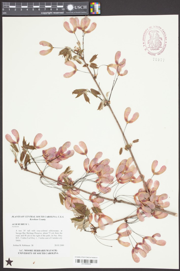
An example of a herbarium specimen used in analysis showing stage 5 of the eight‐stage scheme for reproduction and stage 2 for leafing out. Accessed from https://www.idigbio.org/portal/search and also available at http://sernecportal.org/portal/collections/individual/index.php?occid=9308514.

To capture phenology, each specimen was given a reproductive phenology score (i.e., the stage of flowers or fruits visible) based on a 10‐point scale ranging from no sign of reproduction early in the spring (stage 0) to all flowering and seeding concluded (stage 9); as described in Table 1. Specimens were also given a leafing phenology score, based on a five‐point scale, ranging from no leaves (stage 0) to fully mature leaves (stage 4) (Appendix S1). Specimens scored as both reproductive phase 0 or 9 and leaf‐out stage 0 or 4 were not included in these analyses because they represent the time periods before and after reproduction and leafing out.

Table 1.

Phenophase coding schemes for reproductive phenology, illustrating the morphological information used to categorize reproductive phenology into 10 stages. Only specimens categorized in stages 1–8 were used for analyses. Columns 3–5 describe how these eight reproductive stages were assigned to the other categorization schemes utilized in models

Reproductive phenology (flower/fruit category)	Eight‐stage scheme	Four‐stage scheme	Two‐stage scheme	One‐stage scheme
No sign of reproduction, specimen has no leaves	NA	NA	NA	NA
Flowerbuds visible, but immature, unopened	1	bud	flower	repro.
Buds breaking, early‐flowering parts visible	2	flower	flower	repro.
Mature fully extended flowers	3	flower	flower	repro.
Flowers falling off, fruit just visible	4	fruit	fruit	repro.
Flowers gone, fruit is young (flat and/or crinkled)	5	fruit	fruit	repro.
Immature fruit, though fully formed (samaras plump)	6	fruit	fruit	repro.
Fruit mature, samaras just beginning to separate (50% or less)	7	seed	fruit	repro.
Samaras fully separated, more than 50% of fruits have fallen	8	seed	fruit	repro.
No sign of reproduction, specimen fully leafed out	NA	NA	NA	NA

NA = not applicable.

Specimens ranged in collection year from 1832–2016 and were collected from Florida, USA, to Newfoundland, Canada (Fig. 2). As is common, the herbarium specimens in this study were not evenly distributed in their collection locations (e.g., Daru et al., 2018). Specimens were concentrated in the coastal region of the northeastern United States, northern Florida, the southern Appalachians, and an arc running from southern Louisiana to eastern Missouri (Fig. 2). It is difficult to know if or how this bias impacted our results. We encourage future collection in areas with few specimens.

Figure 2.

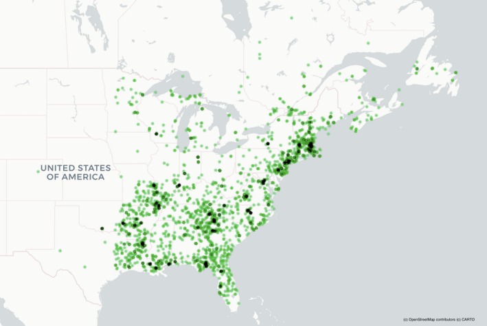
Map showing collection localities of herbarium specimens used in this research. Green dots indicate where a specimen was collected and darker areas indicate a greater number of specimens from that locality.

To relate reproductive phenology to climate, we calculated mean monthly January, February, and March temperature from climate stations within 25 km of each specimen collection locality, for the year in which the specimen was collected. An alternative variable for this analysis would be growing degree days; however, it has been demonstrated that temperature is a robust proxy for degree‐day accumulation (Basler, 2015). Mean temperatures have the major advantage of being more intuitively understandable. This timeframe of January to March was selected to account for early phenology in the southern part of the range and later phenology in the north. Because of the wide geographic range of the specimens, our approach likely misses months that are relevant to the phenology of some specimens, but represents a minimal time period during which many phenophases occur while still maintaining a focus on the early part of the growing season. In effect, this temperature value is an estimate of the climate in the place and year in which a specimen was collected.

To collect historic climate data for each specimen, we used a combination of the R packages ggmap (Kahle and Wickham, 2013) and rnoaa (Chamberlain, 2017). First, we supplemented existing geospatial data by adding latitude and longitude coordinates for specimens that lacked them. We used the “geocode” function in ggmap, which references known location data (address, city, county) against the Google Maps API. Specimens without geospatial data were assigned a latitude and longitude with increasing generalization based on available location records (address > city > county). Specimens assigned geospatial data based on city or county were given the latitude and longitude at the centroid of the political unit.

Next, for each specimen, we identified the nearest weather station in the National Oceanic and Atmospheric Administration's Global Historical Climatology Network with available temperature data for the year the specimen was collected. The station search was limited to within a 25‐km radius of the specimen's collection site. The mean monthly temperature was calculated by first taking the mean of the daily minimum and maximum temperature (to calculate the daily mean temperature), then taking the mean of all daily mean temperatures within the month. Months that did not have any records for minimum and maximum daily temperature or a complete record of daily temperatures for the entire month were excluded.

Elevation data were extracted for each specimen with available geospatial data from the United States Geological Survey (USGS) Global Multi‐Resolution Terrain Elevation 2010 data set at 30‐second‐arc resolution (Danielson and Gesch, 2011).

Classification schemes

To address our research questions, we first established a series of categorizations focused on the reproductive phenophases:

Eight‐stage scheme: The most detailed categorization included stages 1–8, excluding those specimens in stages with no reproductive structures present (henceforth, eight‐stage scheme; Table 1).

Four‐stage scheme: We next created a category using a coarser‐scale categorization by converting our eight‐stage scheme to a four‐stage scheme that mimics several large‐scale citizen science phenological monitoring projects, such as USA National Phenology Network and Project BudBurst (Henderson et al., 2012; http://www.budburst.org). Specifically, we classified the reproductive stage 1 as “bud,” stages 2 and 3 were combined as “flower,” stages 4, 5, and 6 were combined as “fruit,” and stages 7 and 8 were combined as “seed” (four‐stage scheme).

Two‐stage scheme: We then tested a phenological categorization scheme at an even coarser scale that mimics the two‐stage phenological coding system often employed by herbaria. Here, stages 1–3 were combined as “flower” and stages 4–8 were combined as “fruit” (two‐stage scheme).

One‐stage scheme: In the most reduced model, all reproductive stages were considered in a single “reproductive” stage (one‐stage scheme).

Specimens were coded only once, based on the eight‐stage scheme, and then the data set was analyzed with various stages combined (Table 1). It is possible that recategorizing specimens based specifically on the criteria of each scheme, i.e., assessing and categorizing each specimen repeatedly, once for each scheme, could eliminate dependency on the initial data set; however, we are confident that analyses based on the initial data set are robust to our combinations.

Statistical analysis

To address our first two questions—whether finer‐scale phenophases improve our understanding of variation in reproductive phenology and the effects of climate on reproductive phenology—we compared models fit to data with each of these four categorization schemes, using the Akaike information criterion (AIC) to determine which provided the best balance between model fit and parsimony, and R ² values to assess the loss of information from less detailed phenological categorization schemes. Models included the date of collection as the response variable, and four explanatory variables: one of the four phenological categorization schemes (i.e., the phenophase of the specimen—a factor with eight, four, two, or one levels depending on the scheme), temperature (average January, February, and March temperature in Celsius from the nearest weather station), the year the specimen was collected, and elevation (in meters). We included year in the models to assess if and how phenology was shifting over time. It is well understood that plant phenology is largely impacted by temperature, particularly in temperate ecosystems, and including year in our models provided a variable by which to evaluate phenological shifts beyond those accounted for by temperature alone. These models are comparable to those in other published phenological studies (e.g., Gallinat et al., 2018).

We fit models including only one two‐way interaction (between temperature and reproductive phenophase—implying phenophase‐specific responses to temperature), as three‐ and four‐way interactions can be difficult to interpret. Additionally, we were primarily interested in interactions between our phenological categorization scheme and the other explanatory variables, and preliminary model selection (Appendix S2) suggested this two‐way interaction had most support. We next examined the significance and direction of coefficients describing the effects of these explanatory variables across the four models, to determine how our understanding of reproductive phenology would have been altered by less detailed information on reproductive phenology. These analyses were based on 1051 total specimens (the full set of 2945 specimens minus those that did not show stages of reproduction and leaf‐out, and those without adequate label information—e.g., location or date).

To address our third question—whether more detailed information on reproductive and leafing out phenology alters our understanding of the co‐occurrence of these two events—we compared the timing of reproductive phenology to the timing of leaf development, using the same four phenophase categorization schemes described above. First, we conducted three correlation tests (using Kendall's tau coefficient) to ask whether using less detailed categorizations of reproductive phenology alters our ability to detect covariation between flowering and early fruiting and leafing out (which both occur early in the growing season for this species). As these correlations did not require climate or location data, these analyses were conducted using a larger data set (1548 specimens) than analyses linking climate and reproductive and leafing phenology.

Next, we compared the effects of temperature on reproductive vs. leafing phenology. We did this by first determining the relationship between climate, elevation, year, and leafing phenology in similar models as we fit for reproductive phenology. Specifically, we fit a linear model with date of collection as the response variable, the leafing phenophase of the specimen (factor with three levels), temperature (average January, February, and March temperature in Celsius from the nearest weather station), the year the specimen was collected, and elevation (in meters). We fit these models including only one two‐way interaction (between elevation and leafing phenophase), which preliminary model selection indicated had the most support (Appendix S3). We then used model output to test the hypothesis that the coefficient describing temperature effects on leafing phenology from this model differs from that describing temperature effects on reproductive phenology (for each of the four categorization schemes).

Because the effects of temperature on reproductive phenology depended on the reproductive stage (i.e., there was an interaction between reproductive phenophase and temperature), we proceeded with two approaches. First, we used a Wald test to test whether the coefficient describing the effect of temperature on reproductive phenology (in a model where temperature effects on the timing of a phenophase did not differ by stage) differed from the coefficient describing the effect of temperature on leafing phenology. We next used a Wald test to assess whether the phenophase‐specific effects of temperature on reproductive phenology differed from the effect of temperature on leafing phenology, as estimated from the temperature coefficient in the leafing model.

All analyses were completed using R statistical software, version 3.5.0 (R Core Team, 2018).

Results

We found strong support for more detailed reproductive phenology classification schemes, with ΔAIC of the eight‐stage scheme between 45 and 670, as compared to the three simpler classification schemes (Table 2). Post‐hoc tests also demonstrated significant differences in the timing of most (but not all) of the eight reproductive phenophases (Appendix S4). However, R ² values associated with the four‐stage (0.73) and two‐stage phenology (0.69) classification schemes were not substantially lower than the eight‐stage scheme (0.75) (Table 2), suggesting that more of the variation in the data is explained by explanatory variables other than detailed categories of phenophases.

Table 2.

Insights gained from fitting four models using different reproductive phenology classification schemes (from very detailed in the second column to least detailed in the fifth column) to the same data. All models had date of collection as response variable and reproductive stage, elevation, year, temperature, and the interaction between temperature and reproductive stage as explanatory variables. Shown are estimates of elevation, year, and temperature effects (by reproductive stage), Akaike information criterion (AIC) values, ΔAIC values, and R ² values from each model

Model output	Reproductive phenology categorization scheme
	Eight‐stage scheme	Four‐stage scheme	Two‐stage scheme	One‐stage scheme
Model coefficients
Elevation (km)	2.73	2.97	2.827	4.252
Year (decades)	−1.261	−1.290	−1.457	−1.479
Temperature*phenophase	−2.387 (Stage 1) −3.751 (Stage 2) −4.041 (Stage 3) −4.093 (Stage 4) −4.869 (Stage 5) −5.225 (Stage 6) −5.267 (Stage 7) −5.065 (Stage 8)	−2.381 (bud) −3.850 (flower) −4.589 (fruit) −5.199 (seed)	−3.573 (flower) −4.981 (fruit)	−4.154
AIC	8897.68	8943.53	9099.77	9570.17
ΔAIC	0	45.85	202.09	672.49
R 2	0.748	0.733	0.687	0.509

All four reproductive phenology classification schemes provided strong evidence that temperature, elevation, and year influence reproductive phenology in expected ways (Table 2). This was the case even for the one‐stage model in which the specimens were just classified as to whether or not they had reproductive structures. For example, reproductive phenology advanced for each degree Celsius of warming (ranging from 2.3 to 5.2 days [Table 2], depending on the phenological phase and reproductive phenology classification scheme); given that temperature varied by 30°C in this study, this means that flowering could be 120 days earlier and fruit maturation could be 150 days earlier in the warmest locations in comparison with the coldest locations. Similarly, reproduction was delayed at higher elevations (ranging from a delay of 2.70 to 4.30 days per kilometer), or about five to eight days across the elevation range of this region. And finally, reproduction occurred earlier in more recent years, advancing by 13 to 15 days over the past 100 years. All models with multiple phenophases demonstrated that effects of temperature were stronger on later phenophases than on earlier phenophases, implying that the entire process of reproduction (from bud to mature fruit) occurred more rapidly in warmer climates (about three weeks) than in colder climates (about 10 weeks) (Fig. 3).

Figure 3.

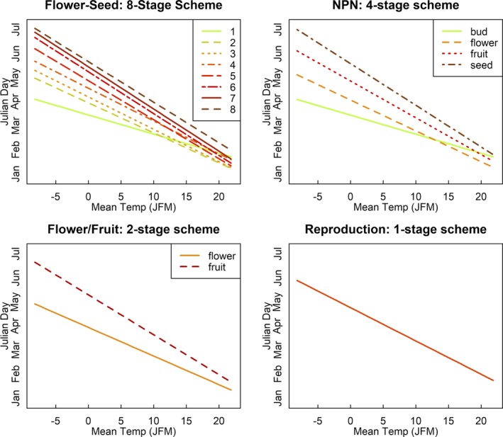
Relationship between mean January, February, and March temperatures (JFM) and the collection dates of herbarium specimens with reproductive structures, according to one of the four classification schemes. The slope of each line represents the effect that warmer spring temperatures have on the timing of reproductive phenology. NPN = USA National Phenology Network.

As with reproductive phenology, we found strong support that leafing phenology advances in warmer temperatures, at lower elevation, and in recent years (Table 3). Correlations demonstrated that leafing phenology and reproductive phenology co‐occurred (Kendall's tau > 0.55 for all phenological categorization schemes). There were relatively few flowering A. rubrum trees with fully mature leaves, and most seeding A. rubrum trees had fully mature leaves (Appendix S5). However, models also demonstrated that the timing of reproduction, especially of later reproductive phenophases, had a stronger negative correlation with temperature than did leafing out phenology (Table 4, Appendix S6). The differences in the effects of temperature on leafing vs. reproductive phenology were significant for all but the earliest reproductive phenophases (Table 4). This difference emerged regardless of the reproductive phenological categorization scheme employed, and means that flowering sometimes occurred weeks ahead of leafing out in the warmest, southern locations, but at about the same time as leafing out in colder, northern locations (Appendix S6).

Table 3.

Comparison of temperature, elevation, and year effects on reproductive phenology (second column) vs. leafing phenology (third column). Shown are coefficients describing the effects of each explanatory variable on the timing of reproduction vs. timing of leafing out. For reproductive phenology, only coefficients from the eight‐stage categorization scheme (identical to those in Table 2) are presented for simplicity

Model coefficients	Phenological event
	Reproductive phenology	Leaf phenologya
Elevation (km)	2.73	9.90 (Leaf Stage 1)
	NA	6.10 (Leaf Stage 2)
	NA	2.60 (Leaf Stage 3)
Year (decades)	−1.261	−1.222
Temperature*phenophase	−2.387 (Stage 1)	−3.371
	−3.751 (Stage 2)	NA
	−4.041 (Stage 3)	NA
	−4.093 (Stage 4)	NA
	−4.870 (Stage 5)	NA
	−5.225 (Stage 6)	NA
	−5.267 (Stage 7)	NA
	−5.065 (Stage 8)	NA

^aNA refers to coefficients not included in best‐fit models for reproductive phenology or leafing phenology. For example, reproductive phenology models included an interaction between temperature and phenophase (implying a stage‐specific effect of temperature), but best‐fit models for leafing phenology did not.

Table 4.

Implications of using differing reproductive phenology categorizations on our ability to detect differences in temperature effects on reproductive vs. leafing phenology. We report hypothesis tests of models that do not allow temperature effects to vary across phenophases (test 1), as well as P values associated with tests of whether stage‐specific effects of temperature on reproduction differ from the effect of temperature on leafing (test 2). Test 2 shows that temperature effects on reproduction are different from temperature effects on leafing for all but the earliest reproductive stages

H(JFMr = JFMl)	Reproductive phenology categorization scheme
	Eight‐stage scheme	Four‐stage scheme	Two‐stage scheme	One‐stage scheme
Test 1: models with temperature effects equivalent across stages	P < 0.0001	P < 0.0001	P < 0.0001	P < 0.0001
Test 2: models with stage‐specific effects of temperature	P = 0.0860 (Stage 1) P = 0.0330 (Stage 2) P = 0.0104 (Stage 3) P = 0.0140 (Stage 4) P = 0.0002 (Stage 5) P < 0.0001 (Stage 6) P < 0.0001 (Stage 7) P < 0.0001 (Stage 8)	P = 0.0923 (bud) P = 0.0186 (flower) P = 0.0004 (fruit) P < 0.0001 (seed)	P = 0.3581 (flower) P < 0.0001 (fruit)	NA

NA = not applicable.

Discussion

Plant reproduction is a process that starts at the first sign of buds and does not finish until the dispersal of the last seed. Our statistical models provide strong support that categorizing this continuous process into eight stages (phases) explains more variation than fewer stages in reproductive phenology of A. rubrum. However, our analyses also demonstrate that less detailed classifications of reproductive phenology, such as four stages and two stages, would have allowed us to gain many of the same insights with respect to the link between climate and reproductive phenology. Thus, in situations where the cost of collecting more detailed information could be significant, less detailed classification schemes will likely suffice. We discuss these results in more detail below.

Do finer‐scale categorizations of reproductive phenology better explain variation in reproductive phenology?

Our analyses of reproductive phenology at varying levels of detail demonstrate that fine‐scale phenological categorizations provided the best‐fit estimate of phenological time and explain more variation than models using coarser‐scale categorizations (see AIC and R ² values in Table 2). This implies that despite the many sources of variation we cannot capture (e.g., tree‐to‐tree differences, observer error, topographic and microsite variation within geographical units), the different morphological stages we scored on herbarium specimens do represent phases that statistically occur at different times (Fig. 3, Appendix S4). At the same time, the difference in how well models with the most detailed categorization (the eight‐stage scheme) performed relative to models with less detailed reproductive phenology schemes accounted for a relatively small amount of variation (see R ² values in Table 2); even though the improvement in the model was real, it was small. Further evidence that these findings are robust can be found in Pearson (2019), in which the author came to a similar conclusion using simulated data sets.

Does more detailed reproductive classification improve our understanding of the link between climate and reproductive phenology?

Many ecologists study phenology to explore the biological impacts of climate change; thus, an important question is whether our most detailed reproductive phenology classification scheme provided us insights into reproductive phenology that we otherwise could not have captured. In fact, all of our reproductive phenology classification schemes demonstrated that reproduction happens earlier in warmer climates and at lower elevations and is shifting earlier over the past century (Fig. 2, Table 2). Thus, if the goal of a phenological study is to assess how phenology, and possibly plant success, is impacted by rising temperatures or varies with elevation, or how it is shifting over time due to warming temperatures and other climatic changes, the additional effort of using a more finely divided phenological system may not be needed. For red maple, we found that the four‐stage reproductive phenology classification scheme commonly used in many professional and citizen science efforts (e.g., the USA National Phenological Network) provided a good balance between detail and simplicity, although the two‐stage classification used by herbaria (flowers, fruit) was almost as effective at demonstrating the effects of climate, elevation, and year on reproductive phenology. This is consistent with the results of a multiple range test, which illustrates that many, but not all, of the eight phenological phases scored differ from each other in terms of collection dates (Appendix S4).

Of course, our study focused on just one tree species (red maple, A. rubrum), so it is important to consider whether collecting more detailed reproductive phenology data might be preferable for other species. Field studies have observed that variations in climate can differentially impact particular phenophases of alpine species (CaraDonna et al., 2014), suggesting that such detailed data collection may be warranted under some circumstances. In our study, red maple herbarium data were gathered over a large geographical area (reflecting the wide distribution of this species) in which there are strong latitudinal and elevation gradients in climate, and over a 180‐year period during which temperatures have increased across the region. This meant that most of the variation in our collection date data was explained by climate, not the reproductive classification scheme we used (R ² values in Table 2). More detailed reproductive phenology classification schemes could prove more useful when studying species with a narrower geographical range that experience less variation in climate across their ranges, or are collected over a shorter period of time. Conversely, it is possible that smaller sample sizes associated with species with more narrow distributions or collected over shorter periods of time might lead to more noise in the model, which could reduce the benefit of finer‐scale categorization of phenophases. Based on a preliminary analysis, however, we found our conclusions to be highly robust to sample size, to the point that we were able to recover our main results even with a 95% reduction in sample size (Appendix S7). Additionally, red maple has relatively rapid fruit development (flowering to seed set occurs over 3–6 weeks). Species with longer fruit development times might benefit from more detailed reproductive phenology classification schemes to better understand how the duration of reproduction might vary with gradients of interest (e.g., climate in Fig. 3). These topics would be worthy of further research and analysis.

Does a more detailed reproductive classification improve our understanding of the co‐occurrence between reproduction and leafing out?

For red maple, spring leaf‐out occurs at roughly the same time as flowering and fruiting or somewhat later (Tables 3, 4; Appendices S5, S6). Unexpectedly, analyses also revealed that flowering in red maples is more responsive to temperature than leafing out. Specifically, red maple trees start to flower weeks or even months before leaf‐out occurs in the southern part of their range, in contrast to the northern parts of their range, where flowering starts only slightly earlier or at the same time as leafing out. This varying phenological response suggests that leaf buds and flower buds have somewhat different physiological mechanisms for responding to their environment, in contrast to the alternative viewpoint that flowering and leafing have similar methods for the control of spring phenology. This could be investigated further in studies of factors controlling leaf and flower buds (Zohner and Renner, 2015). Regardless of the mechanism, our study demonstrates that collecting both types of phenological data provides a more complete picture of how reproductive phenology varies with climate.

However, just as with analyses of the effects of climate, elevation, and year on reproductive phenology, insights about the co‐occurrence of reproductive and leafing phenology did not depend on using the most detailed reproductive phenology classification scheme. Specifically, pairwise correlations between reproductive phenology and leafing phenology were strongly positive and significant for the eight‐stage, four‐stage, and two‐stage reproductive phenology classification schemes. The different effects of temperature on leafing vs. reproductive phenology were as evident when applying the four‐stage and two‐stage reproductive phenology classification scheme as they were when using the eight‐stage reproductive phenology classification scheme. In short, our results demonstrate that any reproductive phenology classification scheme that separates earlier stages of reproduction (flowering) from later phases (young fruit and mature fruit) could have captured the difference in the timing of these events relative to leaf‐out in the warm vs. cold portions of this species range.

Implications of our study for ongoing efforts to study phenology using citizen science

Global efforts to digitize natural history collections have made it possible for images of millions of specimens to be viewed and evaluated by citizen scientists—e.g., through online tools like CrowdCurio (http://www.crowdcurio.com) and Notes from Nature (https://www.notesfromnature.org)—thereby creating the potential for huge amounts of digital data to be available to researchers (Ellwood et al., 2015). As we consider scalability of our methods and look to expand this method to other taxa, incorporating online citizen scientists into the workflow can be a way to greatly advance our efforts. Given that we found support for finer‐scale classifications of reproductive phenology, even if the improvement in explanatory power was small, one might surmise that it would be best to ask those digitizing specimens to categorize phenology at the most detailed scale possible.

However, the trade‐off between the time and resources necessary to reliably categorize specimens at such fine scales may not be worth the small improvements in information and explanatory power of analytical models. In our classification workflow, we carefully evaluated and recorded the reproductive and leafing phenophases of each herbarium specimen based on a detailed rubric. For citizen scientists not trained in botany, this fine‐scale categorization would likely require substantial training and resources—such as detailed descriptions and photos of the phenological stages of each species—and quality control mechanisms. This training and quality control would require substantial time and investment for relatively little benefit in information. Our study suggests that the four‐stage classification scheme of reproductive phenology is suitable for addressing the most central phenological questions, and that even a two‐stage scheme is strong, thereby providing support for coarse‐level evaluations by citizen scientists without extensive training (Tables 2, 3; Fig. 3). At the same time, our results also demonstrate asking citizen scientists to categorize multiple reproductive phenological events on the same specimen (e.g., reproduction, leafing out) can add a great deal of information and provide important insights (Table 4, Appendix S6).

Summary

Our study demonstrates that finer‐scale categorization of phenological stages results in more robust models of the relationship of phenology to climate, elevation, and advancing years. However, we also show that more simple systems of classification, including even a two‐stage system of flowers and fruit, provide very similar results. We recognize that our approach might not be applicable to plants with categorically different reproductive systems and life histories. Indeed, for some species it may be impossible to acquire phenological data from herbarium specimens. Nonetheless, we believe that our results have general applicability to species with a similar ecology to red maple, including most common temperate, deciduous trees and shrubs, and encourage further research testing these questions within a diversity of species. Such simple systems of classification offer further advantages in terms of being easy for citizen scientists to learn and to use, and are probably less prone to classification errors.

Supporting information

APPENDIX S1. Description of morphological features used to code Acer rubrum herbarium specimens. Note only stages 1, 2, and 3 were used in analyses presented in the main text.

APPENDIX S2. Model selection results for linear models including different combinations of two‐way interactions between reproductive phenophase and temperature, elevation, and/or year.^a

APPENDIX S3. Model selection results for linear models including different combinations of two‐way interactions between leafing phenophase and temperature, elevation, and/or year.^a

APPENDIX S4. Timing of different reproductive stages and leafing stages, as predicted by best fitting models at the mean elevation (545 m), year (1946), and January, February, or March temperature (8.35°C) in our data set.

APPENDIX S5. Co‐occurrence of reproductive (y‐axis) and leafing (top x‐axis) phenophases; overall (left), in northern states (>42.5° latitude, center), and in southern states (<32.5° latitude, right).

APPENDIX S6. Comparison of the effects of temperature on the timing of flowering, seed set, and leafing out.

APPENDIX S7. Sensitivity analysis of classification scheme model‐fit to sample size.

Ellwood, E. R. , Primack R. B., Willis C. G., and J. HilleRisLambers . 2019. Phenology models using herbarium specimens are only slightly improved by using finer‐scale stages of reproduction. Applications in Plant Sciences 7(3): e1225.

Data Accessibility

Our data set of Acer rubrum phenology, as well as the code we created to run the analyses described here, are available at https://github.com/cgwillis/AcerPhenologyProject.

Literature Cited

- Andrew, C. , Büntgen U., Egli S., Senn‐Irlet B., Grytnes J.‐A., Heilmann‐Clausen J., Boddy L., et al. 2019. Open‐source data reveal how collections‐based fungal diversity is sensitive to global change. Applications in Plant Sciences 7(3): e1227. [DOI] [PMC free article] [PubMed] [Google Scholar]
- Bartomeus, I. , Ascher J. S., Wagner D., Danforth B. N., Colla S., Kornbluth S., and Winfree R.. 2011. Climate‐associated phenological advances in bee pollinators and bee‐pollinated plants. Proceedings of the National Academy of Sciences USA 108: 20645–20649. [DOI] [PMC free article] [PubMed] [Google Scholar]
- Basler, D. 2015. Evaluating phenological models for the prediction of leaf‐out dates in six temperate tree species across central Europe. Agricultural and Forest Meteorology 217: 10–21. [Google Scholar]
- CaraDonna, P. J. , Iler A. M., and Inouye D. W.. 2014. Shifts in flowering phenology reshape a subalpine plant community. Proceedings of the National Academy of Sciences USA 111: 4916–4921. [DOI] [PMC free article] [PubMed] [Google Scholar]
- Carranza‐Rojas, J. , Goeau H., Bonnet P., Mata‐Montero E., and Joly A.. 2017. Going deeper in the automated identification of herbarium specimens. BMC Evolutionary Biology 17: 181. [DOI] [PMC free article] [PubMed] [Google Scholar]
- Chamberlain, S. 2017. rnoaa: ‘NOAA’ Weather Data from R. R package version 0.7.0. Website https://cran.r-project.org/web/packages/rnoaa/ [accessed 15 January 2018].
- Cook, B. I. , and Wolkovich E. M.. 2016. Climate change decouples drought from early wine grape harvests in France. Nature Climate Change 6: 715. [Google Scholar]
- Danielson, J. J. , and Gesch D. B.. 2011. Global multi‐resolution terrain elevation data 2010 (GMTED2010): U.S. Geological Survey Open‐File Report 2011–1073. Earth Resources Observation and Science (EROS) Center, U.S. Geological Survey, Sioux Falls, South Dakota, USA.
- Daru, B. H. , Park D. S., Primack R. B., Willis C. G., Barrington D. S., Whitfeld T. J. S., Seidler T. G., et al. 2018. Widespread sampling biases in herbaria revealed from large‐scale digitization. New Phytologist 217: 939–955. [DOI] [PubMed] [Google Scholar]
- Davis, C. C. , Willis C. G., Connolly B., Kelly C., and Ellison A. M.. 2015. Herbarium records are reliable sources of phenological change driven by climate and provide novel insights into species’ phenological cueing mechanisms. American Journal of Botany 102: 1599–1609. [DOI] [PubMed] [Google Scholar]
- Denny, E. G. , Gerst K. L., Miller‐Rushing A. J., Tierney G. L., Crimmins T. M., Enquist C. A. F., Guertin P., et al. 2014. Standardized phenology monitoring methods to track plant and animal activity for science and resource management applications. International Journal of Biometeorology 58: 591–601. [DOI] [PMC free article] [PubMed] [Google Scholar]
- Diskin, E. , Proctor H., Jebb M., Sparks T., and Donnelly A.. 2012. The phenology of Rubus fruticosus in Ireland: Herbarium specimens provide evidence for the response of phenophases to temperature, with implications for climate warming. International Journal of Biometeorology 56: 1103–1111. [DOI] [PubMed] [Google Scholar]
- Ellwood, E. R. , Dunckel B. A., Flemons P., Guralnick R., Nelson G., Newman G., Newman S., et al. 2015. Accelerating the digitization of biodiversity research specimens through online public participation. BioScience 65: 383–396. [Google Scholar]
- Everill, P. H. , Primack R. B., Ellwood E. R., and Melaas E. K.. 2014. Determining past leaf‐out times of New England's deciduous forests from herbarium specimens. American Journal of Botany 101: 1293–1300. [DOI] [PubMed] [Google Scholar]
- Gallinat, A. S. , Russo L., Melaas E. K., Willis C. G., and Primack R. B.. 2018. Herbarium specimens show patterns of fruiting phenology in native and invasive plant species across New England. American Journal of Botany 105: 31–41. [DOI] [PubMed] [Google Scholar]
- Henderson, S. , Ward D. L., Meymaris K. K., Alaback P., and Havens K.. 2012. Project Budburst: Citizen science for all seasons In Dickinson J. L. and Bonney R. [eds.], Citizen science: Public participation in environmental research, 50–57. Cornell University Press, Ithaca, New York, USA. [Google Scholar]
- Kahle, D. , and Wickham H.. 2013. ggmap: Spatial visualization with ggplot2. R Journal 5: 144–161. [Google Scholar]
- Lorieul, T. , Pearson K. D., Ellwood E. R., Goëau H., Molino J.‐F., Sweeney P. W., Yost J. M., et al. 2019. Toward a large‐scale and deep phenological stage annotation of herbarium specimens: Case studies from temperate, tropical, and equatorial floras. Applications in Plant Sciences 7(3): e1233. [DOI] [PMC free article] [PubMed] [Google Scholar]
- Meier, U. , Bleiholder H., Buhr L., Feller C., Hack H., Heß M., Lancashire P. D., et al. 2009. The BBCH system to coding the phenological growth stages of plants—History and publications. Journal für Kulturpflanzen 61: 41–52. [Google Scholar]
- Munson, S. M. , and Long A. L.. 2017. Climate drives shifts in grass reproductive phenology across the western USA. New Phytologist 213: 1945–1955. [DOI] [PubMed] [Google Scholar]
- Panchen, Z. A. , Primack R. B., Aniśko T., and Lyons R. E.. 2012. Herbarium specimens, photographs, and field observations show Philadelphia area plants are responding to climate change. American Journal of Botany 99: 751–756. [DOI] [PubMed] [Google Scholar]
- Pearson, K . 2019. A new method and insights for estimating phenological events from herbarium specimens. Applications in Plant Sciences 7(3): e1224. [DOI] [PMC free article] [PubMed] [Google Scholar]
- R Core Team . 2018. R: A language and environment for statistical computing. R Foundation for Statistical Computing, Vienna, Austria. [Google Scholar]
- Rawal, D. S. , Kasel S., Keatley M. R., and Nitschke C. R.. 2015. Herbarium records identify sensitivity of flowering phenology of eucalypts to climate: Implications for species response to climate change. Austral Ecology 40: 117–125. [Google Scholar]
- Renner, S. S. , and Zohner C. M.. 2018. Climate change and phenological mismatch in trophic interactions among plants, insects, and vertebrates. Annual Review of Ecology, Evolution, and Systematics 49: 165–182. [Google Scholar]
- Spellman, K. V. , and Mulder C. P. H.. 2016. Validating herbarium‐based phenology models using citizen‐science data. BioScience 66: 897–906. [Google Scholar]
- Tang, J. , Körner C., Muraoka H., Piao S., Shen M., Thackeray S. J., and Yang X.. 2016. Emerging opportunities and challenges in phenology: A review. Ecosphere 7: e01436. [Google Scholar]
- Willis, C. G. , Law E., Williams A. C., Franzone B. F., Bernardos R., Bruno L., Hopkins C., et al. 2017a. CrowdCurio: An online crowdsourcing platform to facilitate climate change studies using herbarium specimens. New Phytologist 215: 479–488. [DOI] [PubMed] [Google Scholar]
- Willis, C. G. , Ellwood E. R., Primack R. B., Davis C. C., Pearson K. D., Gallinat A. S., Yost J. M., et al. 2017b. Old plants, new tricks: Phenological research using herbarium specimens. Trends in Ecology and Evolution 32: 531–546. [DOI] [PubMed] [Google Scholar]
- Wolkovich, E. M. , Cook B. I., and Davies T. J.. 2014. Progress towards an interdisciplinary science of plant phenology: Building predictions across space, time and species diversity. New Phytologist 201: 1156–1162. [DOI] [PubMed] [Google Scholar]
- Zalamea, P.‐C. , Munoz F., Stevenson P. R., Paine C. T., Sarmiento C., Sabatier D., and Heuret P.. 2011. Continental‐scale patterns of Cecropia reproductive phenology: Evidence from herbarium specimens. Proceedings of the Royal Society of London B: Biological Sciences 278: 2437–2445. 10.1098/rspb.2010.2259. [DOI] [PMC free article] [PubMed] [Google Scholar]
- Zohner, C. M. , and Renner S. S.. 2014. Common garden comparison of the leaf‐out phenology of woody species from different native climates, combined with herbarium records, forecasts long‐term change. Ecology Letters 17: 1016–1025. [DOI] [PubMed] [Google Scholar]
- Zohner, C. M. , and Renner S. S.. 2015. Perception of photoperiod in individual buds of mature trees regulates leaf‐out. New Phytologist 208: 1023–1030. [DOI] [PubMed] [Google Scholar]
Associated Data
This section collects any data citations, data availability statements, or supplementary materials included in this article.
Supplementary Materials