

Abstract
Classical bridge regression is known to possess many desirable statistical properties such as oracle, sparsity, and unbiasedness. One outstanding disadvantage of bridge regularization, however, is that it lacks a systematic approach to inference, reducing its flexibility in practical applications. In this study, we propose bridge regression from a Bayesian perspective. Unlike classical bridge regression that summarizes inference using a single point estimate, the proposed Bayesian method provides uncertainty estimates of the regression parameters, allowing coherent inference through the posterior distribution. Under a sparsity assumption non the high-dimensional parameter, we provide sufficient conditions for strong posterior consistency of the Bayesian bridge prior. On simulated datasets, we show that the proposed method performs well compared to several competing methods across a wide range of scenarios. Application to two real datasets further revealed that the proposed method performs as well as or better than published methods while offering the advantage of posterior inference.
Keywords: Bayesian Regularization, Bridge Regression, LASSO, MCMC, Scale Mixture of Uniform, Variable Selection
1. Introduction
In a normal linear regression setup, we have the following model
where y is the n × 1 vector of centered responses, X is the n × p matrix of standardized regressors, βis the p × 1 vector of coefficients to be estimated, and ϵ is the n × 1 vector of independent and identically distributed normal errors with mean 0 and variance ˙σ2. Consider bridge regression (Frank and Friedman, 1993) that results from the following regularization problem
| (1) |
where λ> 0 is the tuning parameter that controls the degree of penalization and α> 0 is the concavity parameter that controls the shape of the penalty function. It is well known that bridge regression includes many popular methods such as best subset selection, LASSO (Tibshirani, 1996), and ridge (Hoerl and Kennard, 1970) as special cases (corresponding to α = 0, α = 1, and α = 2 respectively). Bridge regularization with 0 < α < 1 is known to possess many desirable statistical properties such as oracle, sparsity, and unbiasednesss (Xu et al., 2010). Despite being theoretically attractive in terms of variable selection and parameter estimation, bridge regression usually cannot produce valid standard errors (Kyung et al., 2010). Existing methods such as approximate covariance matrix and bootstrap are known to be unstable for bridge estimator (Knight and Fu, 2000). This means investigators typically must use the resulting bridge estimate without a quantification of its uncertainty.
Bayesian analysis naturally overcomes this limitation by providing a valid measure of uncertainty based on a geometrically ergodic Markov chain with a suitable point estimator. Ideally, a Bayesian solution can be obtained by placing an appropriate prior on the coefficients that will mimic the property of the bridge penalty. Frank and Friedman (1993) suggested that bridge estimates can be interpreted as posterior mode estimates when the regression coefficients are assigned independent and identical generalized Gaussian (GG) priors. While most of the existing Bayesian regularization methods are based on the scale mixture of normal (SMN) representations of the associated priors (Kyung et al., 2010), such a representation is not explicitly available for Bayesian bridge prior when α ϵ (0, 1) (Armagan, 2009; Park and Casella, 2008). Therefore, despite having a natural Bayesian interpretation, a Bayesian solution to bridge regression is not straightforward, which necessitate the exploration of alternative solutions.
Recently, Polson et al. (2014) provided a set of Bayesian bridge estimators for linear models based on two distinct scale mixture representations of the GG density. Among them, one approach utilizes an SMN representation (West, 1987), for which the mixing variable is not explicit in the sense that it requires simulating draws from an exponentially-tilted stable random variable, which is quite di cult to generate in practice (Devroye, 2009). To avoid the need to deal with exponentially tilted stable random variables, Polson et al. (2014) further proposed another Bayesian bridge estimator based on a scale mixture of triangular (SMT) representation of the GG prior. Among the pros and cons of these approaches, it is not clear whether they naturally extend to more general regularization methods such as group bridge (Park and Yoon, 2011) and group LASSO (Yuan and Lin, 2006). There is also limited theoretical work on the Bayesian bridge posterior consistency under suitable assumptions in a sparse high-dimensional linear model.
We address both these issues by providing a flexible approach based on an alternative scale mixture of uniform (SMU) representation of the GG prior, which in turn facilitates computationally efficient Markov chain Monte Carlo (MCMC) algorithm. Consistent with major recently-developed Bayesian penalized regression methods (Kyung et al., 2010), we consider a conditional prior specification on the coefficient, which leads to a simple data-augmentation strategy. Several useful extensions of the method are also presented, providing a unified framework for modeling a variety of outcomes in varied real life scenarios. Further, we investigate sufficient strong posterior consistency conditions of the Bayesian bridge prior, which offers additional insight into the asymptotic behavior of the corresponding posterior distribution.
In summary, we introduce some new aspects of the broader Bayesian treatment of bridge regression. Following Park and Casella (2008), we consider a conditional GG prior (GG distribution with mean 0, shape parameter α, and scale parameter ) of the form
| (2) |
and a non-informative scale-invariant marginal prior on σ2, i.e. π(σ2) α 1/σ2. Rather than minimizing (1), we solve the problem using a Gibbs sampler that involves constructing a Markov chain having the joint posterior for β as its stationary distribution. Unlike classical bridge regression, statistical inference for Bayesian bridge is straightforward. In addition, the tuning parameter can be effortlessly estimated as an automatic byproduct of the MCMC procedure. The remainder of the paper is organized as follows. In Section 2, we describe the hierarchical representation of the proposed Bayesian bridge model. The resulting Gibbs sampler is put forward in Section 3. A result on posterior consistency is presented in Section 4. Some empirical studies and real data analyses are described in Section 5. An Expectation Maximization (EM) algorithm to compute the maximum a posteriori (MAP) estimates is included in Section 6. Some extensions and generalizations are provided in Section 7. Finally, in Section 8, we provide conclusions and further discussions in this area. Some proofs and related derivations are included in a supplementary file.
2. The Model
2.1. SMU Distribution
Propostion 1:
A GG distribution can be written as an SMU distribution, the mixing distribution being a particular gamma distribution as follows
| (3) |
Proof:
Proof of this result is provided in the Supplementary file (Appendix A).
2.2. Hierarchical Representation
Using (2) and (3), we can formulate our hierarchical representation as
| (4) |
3. MCMC Sampling
3.1. Full Conditional Distributions
Introduction of u = (u1, u2, ..., up)′ enables us to derive the full conditional distributions which are given as
| (5) |
| (6) |
| (7) |
where I(.) denotes an indicator function. The proofs involve simple algebra and are omitted.
3.2. Sampling Coefficients And Latent Variables
(5), (6), and (7) lead to a Gibbs sampler that starts at initial guesses of the parameters and iterates the following steps:
- Generate uj from the left-truncated exponential distribution Exp using inversion method, which can be done as follows
- Generate ,
Generate β from a truncated multivariate normal distribution proportional to the posterior distribution of β. This step can be done by implementing efficient sampling technique developed by Li and Ghosh (2015).
Generate σ 2 from a left-truncated Inverse Gamma distribution proportional to (7) which can be done by replacing, where ˙ σ 2* is generated from a right-truncated Gamma distribution (Damien and Walker, 2001; Phillippe, 1997) proportional to
An efficient Gibbs sampler based on these full conditionals proceeds to draw posterior samples from each full conditional posterior distribution, given the current values of all other parameters and the observed data. The process continues until all chains converge.
3.3. Sampling Hyperparameters
To update the tuning parameter λ, we work directly with the GG density, marginalizing out the latent variables uj’s. From (4), we observe that the posterior for λ, given β, is conditionally independent of y. Therefore, if λ has a Gamma (a, b) prior, we can update the tuning parameter by generating samples from its conditional posterior distribution given by
| (8) |
The concavity parameter α is usually prefixed beforehand. Xu et al. (2010) argued that α = 0.5 can be taken as a representative of the Lα , α ϵ (0, 1) regularization. We therefore prefix α to 0.5 in this article. However, it can be estimated by assigning a suitable prior π (α ). Since 0 < α < 1, a natural choice for the prior on α is Beta distribution, which can be updated using a random-walk Metropolis sampler (Polson et al., 2014).
4. Posterior Consistency Under Bayesian Bridge Model
Consider the high dimensional sparse linear regression model where is an n -dimensional vector of responses, Xn is the n × pn design matrix, with known σ2 > 0 and is the true coefficient vector with both zero and non-zero components. To justify high dimensionality, we assume thatas .Let, be the set of non-zero components of and be the cardinality of . Consider the following assumptions as (A1) pn = o(n).
(A2) Let ∧n min and ∧n max be the smallest and largest singular values of Xn respectively. Then,
(A4) for p ∈ (0,2) and α ∈ (0,1).
Armagan et al. (2013) provided sufficient conditions for strong posterior consistency of various shrinkage priors in linear models. Here we extend the results by deriving sufficient conditions for strong posterior consistency of the Bayesian bridge prior using Theorem 1 of Armagan et al. (2013). We re-state the theorem for the sake of completeness.
Theorem 1.
(Armagan et al., 2013) Under assumptions (A1) and (A2), the posterior of under prior ∏ is strongly consistent if
for all and and some p>0
Theorem 2.
Consider the GG prior with mean zero, shape parameter α ϵ (0, 1), and scaleparameter sn > 0 given by
| (9) |
Under assumptions (A1)-(A4), the Bayesian bridge prior (9) yields a strongly consistent posterior if for finite C > 0.
Proof:
Proof of this result is provided in the Supplementary file (Appendix B).
5. Results
In this section, we investigate the prediction accuracy of the proposed Bayesian Bridge Regression (BBR.U) and compare its performance with several published Bayesian and non-Bayesian methods including LASSO (Tibshirani, 1996), Elastic Net (Zou and Hastie, 2005), bridge (Frank and Friedman, 1993), BBR.N, BBR.T, and BLASSO, where BBR.N corresponds to the Bayesian bridge model of Polson et al. (2014) based on the SMN representation of the GG density, BBR.T corresponds to the same based on the SMT representation, and BLASSO corresponds to the Bayesian LASSO model of Park and Casella (2008). For LASSO and elastic net (ENET) solution paths, we use R package glmnet, which implements the coordinate descent algorithm (Friedman et al., 2010) with tuning parameter(s) selected by 10-fold cross-validation. For the classical bridge estimator (BRIDGE), we use R package grpreg, which uses a locally approximated coordinate descent algorithm (Breheny and Huang, 2009) with tuning parameter selected by the generalized cross validation (GCV) criterion (Golub et al., 1979). For BBR.U and BLASSO, we set the hyperparameters as a = 1 and b = 0.1, which leads to a relatively flat distribution and results in high posterior probability near the MLE (Kyung et al., 2010). For BBR.T and BBR.N, a default Gamma (2, 2) prior is used as prior for the tuning parameter, as implemented in the R package Bayes Bridge. Bayesian estimates are posterior means using 10, 000 samples of the Gibbs sampler after burn-in. To decide on the burn-in number, we use the potential scale reduction factor (Ȓ) (Gelman and Rubin, 1992). Once Ȓ < 1.1 for all parameters of interest, we continue to draw 10,000 iterations to obtain samples from the joint posterior distribution. The convergence of the MCMC algorithm is also verified by trace and ACF plots of the generated samples. The response is centered and the predictors are normalized to have zero means and unit variances before applying any model selection method.
5.1. Simulation Experiments
For the simulated examples, we calculate the median of mean squared errors (MMSE) based on 100 replications. Each simulated sample is partitioned into a training set and a test set. Models are fitted on the training set and mean squared errors (MSEs) are calculated based on the held-out samples in the test set. We simulate data from the true model
5.1.1. Simulation 1 (Simple Examples)
Here we investigate the prediction accuracy of BBR.U using three simple models, drawn from published papers (Tibshirani, 1996). Models 1 and 3 represent two di erent sparse scenarios whereas Model 2 represents a dense situation.
Model 1:
Here we set β8×1 = (3, 1.5, 0, 0, 2, 0, 0, 0)T and σ2 = 9. The design matrix X is generated from the multivariate normal distribution with mean 0, variance 1, and pairwise correlations between xi and xj equal to 0.5|i−j| ∀ i ≠ j.
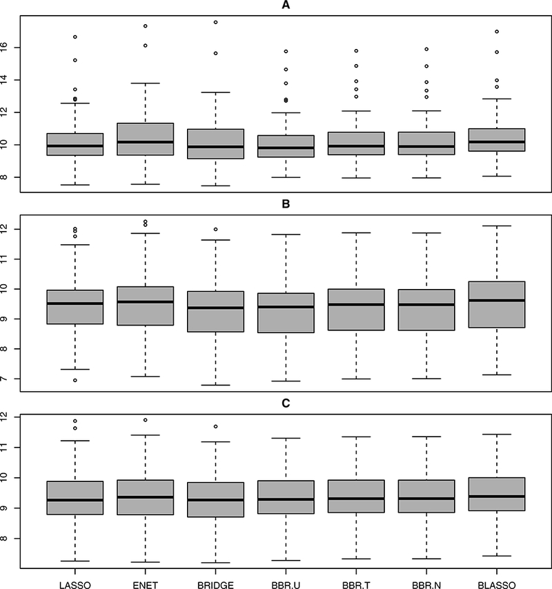
Model 2:
Here we set β8×1 = (0.85, 0.85, 0.85, 0.85, 0.85,0.85, 0.85, 0.85)T , leaving other setups exactly the same as Model 1.
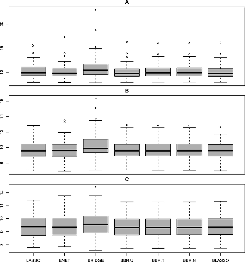
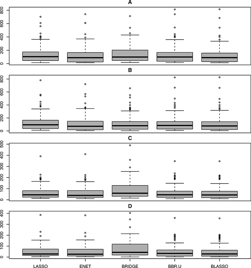
Model 3:
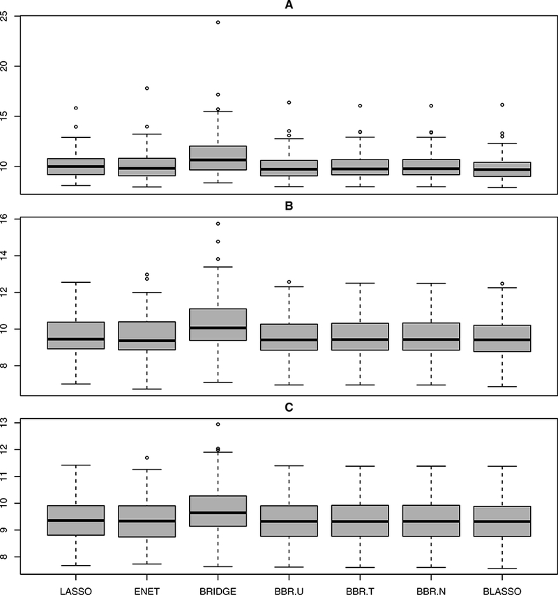
We use the same setup as Model 1 with β8×1 = (5, 0, 0, 0, 0, 0, 0, 0)T . For all the three models, we experiment with three sample sizes n = {50, 100, 200}, referred to as A, B, and C respectively. Prediction error (MSE) was calculated on a test set of 200 observations for each of these cases. The results, presented in Figures 1–3, clearly indicate that BBR.U performs well compared to classical bridge estimator.
Figure 1:
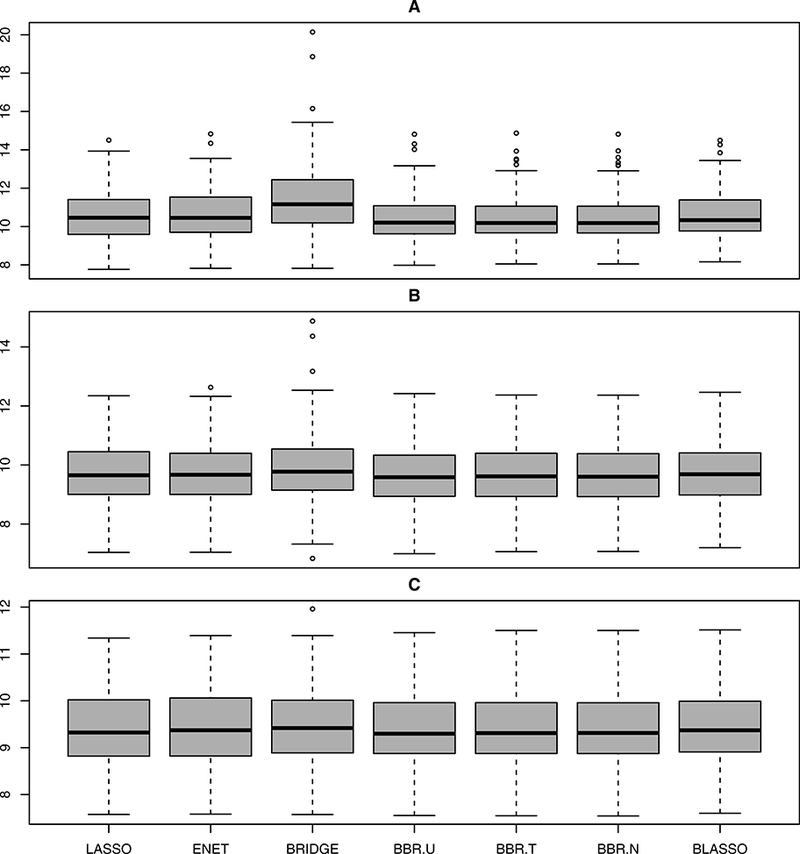
Boxplots summarizing prediction performance of various methods under Model 1.
Figure 3:
Boxplots summarizing the prediction performance of various methods under Model 3.
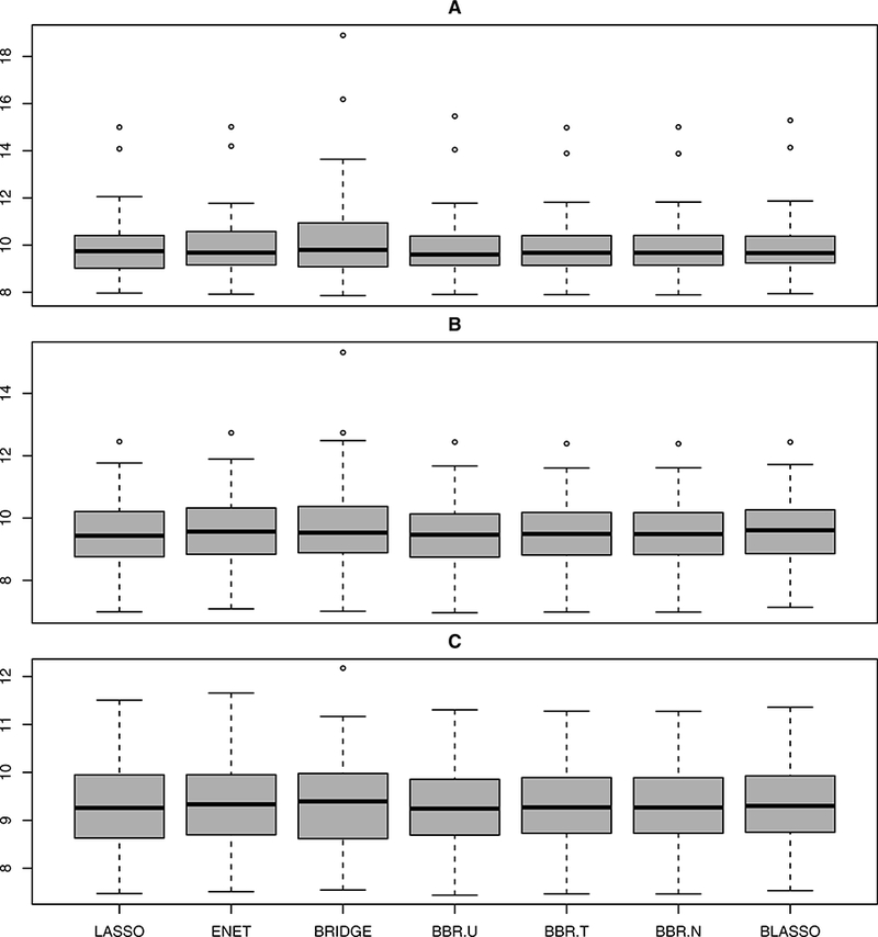
5.1.2. Simulation 2 (High Correlation Examples)
In this simulation study, we investigate the performance of BBR.U in sparse models with strong level of correlation. We repeat the same models in Simulation 1 but experiment with a different design matrix X which is generated from the multivariate normal distribution with mean 0, variance 1, and pairwise correlations between xi and xj equal to 0.95. To distinguish from Simulation 1, we refer to the models in Simulation 2 as Models 4, 5, and 6 respectively. The experimental results, presented in Figures 4–6, reveal that BBR.U performs as well as existing Bayesian methods with better prediction accuracy than frequentist methods.
Figure 4:
Boxplots summarizing the prediction performance of various methods under Model 4.
Figure 6:
Boxplots summarizing the prediction performance of various methods under Model 6.
5.1.3. Simulation 3 (Difficult Examples)
In this simulation study, we evaluate the performance of BBR.U in fairly complicated models, which exhibit a substantial amount of data collinearity.
Model 7:
Here we set β40×1 = (0T, 2T, 0T, 2T )T , where 0 and 2 are vectors of length 10 with each entry equal to 0 and 2 respectively. The design matrix X is generated from the multivariate normal distribution with mean 0, variance 1, and pairwise correlations between xi and xj equal to 0.5. We simulate datasets wih (nT , nP ) ϵ {(100, 400), (200, 200)}, where nT denotes the size of the training set and nP denotes the size of the test set. We consider two values of σ : σ ϵ {9, 25}. The simulation results (Table 1; L, EN, and BL denote LASSO, ENET, and BLASSO respectively) indicate competitive predictive accuracy of BBR.U as compared to published Bayesian methods. In this example, Bayesian methods are marginally outperformed by frequentist methods in specific cases; this could be due to the fact that not much variance is explained by introducing the priors that resulted in slightly worse model selection performance for the Bayesian methods.
Table 1:
MMSE based on 100 replications for Model 7.
| {nT,nP,σ2} | L | EN | BRIDGE | BBR.U | BBR.T | BBR.N | BL |
|---|---|---|---|---|---|---|---|
| {200, 200, 225} | 252.9 | 252.0 | 258.1 | 250.8 | 251.8 | 251.4 | 251.7 |
| {200, 200, 81} | 94.0 | 93.3 | 103.7 | 94.9 | 95.5 | 95.1 | 94.9 |
| {100, 400, 225} | 270.9 | 264.9 | 272.2 | 263.3 | 261.9 | 264.2 | 268.9 |
| {100, 400, 81} | 106.8 | 105.0 | 114.1 | 105.3 | 105.4 | 105.7 | 104.5 |
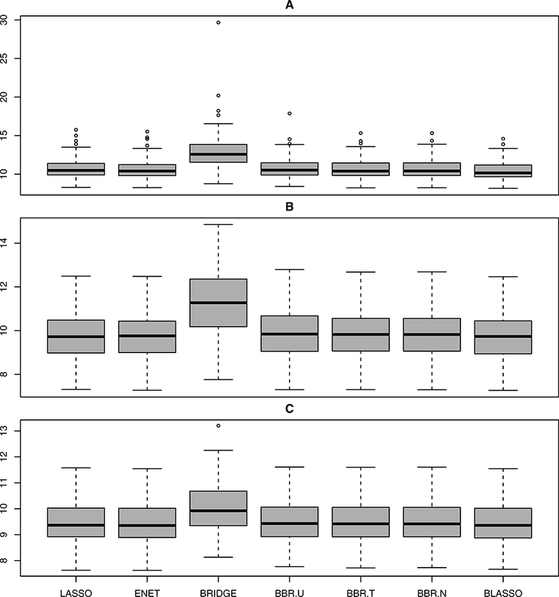
5.1.4. Simulation 4 (Small n Large p Example)
Here we consider a high dimensional case where p ≥ n. We let , p = 20, q = 10, σ ϵ {3, 1}. The design matrix X is generated from the multivariate normal distribution with mean 0, variance 1, and pairwise correlations between xi and xj equal to 0.95
∀ i ≠ j. We simulate datasets with nT ϵ {10, 20} for the training set and nP = 200 for the test set, which we refer to as A (nT = 10, σ = 3), B (nT = 10, σ = 1), C (nT = 20, σ = 3), and D (nT = 20, σ = 1). It is evident that BBR.U always performs better than classical bridge regression (Figure 7). Here we did not include BBR.T and BBR.N as BayesBridge did not converge for most of the scenarios. Taken together, these simulation experiments reveal that Bayesian penalized regression approaches generally outperform their frequentist cousins in estimation and prediction, which is in agreement with an established body of Bayesian regularized regression literature (Kyung et al., 2010; Leng et al., 2014; Mallick, 2015; Mallick and Yi, 2014, 2017; Park and Casella, 2008; Polson et al., 2014).
Figure 7:
Boxplots summarizing the prediction performance of various methods under Model 8.
5.2. Real Data Analyses
Next, we apply these various regularization methods to two benchmark datasets viz. prostate cancer data (Stamey et al., 1989) and pollution data (McDonald and Schwing, 1973). Both these datasets have been used for illustration in previous studies. For both analyses, we randomly divide the data into a training set and a test set. Model fitting is carried out on the training data and performance is evaluated with the prediction error (MSE) on the test data. For both analyses, we also compute the prediction error for the ordinary least squares (OLS) method.
In the prostate cancer dataset, the response variable of interest is the logarithm of prostate-specific antigen. The predictors are eight clinical measures: the logarithm of cancer volume (lcavol), the logarithm of prostate weight (lweight), age, the logarithm of the amount of benign prostatic hyperplasia (lbph), seminal vesicle invasion (svi), the logarithm of capsular penetration (lcp), the Gleason score (gleason), and the percentage Gleason score 4 or 5 (pgg45). We analyze the data by dividing it into a training set with 67 observations and a test set with 30 observations. On the other hand, the pollution dataset consists of 60 observations and 15 predictors. A detailed description of the predictor variables in the pollution dataset is provided in McDonald and Schwing (1973). The response variable is the total age-adjusted mortality rate obtained for the years 1959 − 1961 for 201 Standard Metropolitan Statistical Areas. In order to calculate prediction errors, we randomly select 40 observations for model fitting and use the rest as test set.
We summarize the results for both data analyzes in Tables 2–3, which show that BBR.U performs as well as published Bayesian and non-Baysian methods in terms of prediction accuracy, as measured by both mean squared error (MSE) and mean absolute scaled error (MASE) (Hyndman and Koehler, 2006). We also report the selected variables by each method except OLS, which does not perform automatic variable selection. For the Bayesian methods, we use the 95% credible interval criterion (Park and Casella, 2008) to determine whether a variable is zero or non-zero. We observe that Bayesian methods tend to result in sparser and more parsimonious models, which is consistent with previous studies (Leng et al., 2014). We repeat the random selection of training and test sets many times and obtain the similar result as in Table 2. Figures 8 and 9 describe the 95% equal-tailed credible intervals for the regression parameters of prostate cancer and pollution data respectively, based on the posterior mean Bayesian estimates. To increase the readability of the plots, in each plot, we add a slight horizontal shift to the estimators. We observe that BBR.U gives very similar posterior mean estimates as competing Bayesian methods. It is to be noted that only the Bayesian methods provide valid standard errors for the zero-estimated coefficients. Interestingly, all the estimates are inside the BBR.U credible intervals which indicates that the resulting conclusion will be similar regardless of which method is used. Hence, the analyses show strong support for the use of the proposed method. BBR.U performs similarly for other values of α (data not shown). In summary, BBR.U offers an attractive alternative to existing methods, performing as well as previous methods while offering the advantage of posterior inference.
Table 2:
Summary of prostate data analysis.’MSE’ denotes mean squared error on the test data and ‘MASE’ denotes mean absolute scaled error on the test data.
| Method | Selected Variables | MSE | MASE |
|---|---|---|---|
| OLS | Not applicable | 0.52 | 0.54 |
| LASSO | lcavol, lweight, age, lbph, svi, lcp, pgg45 | 0.49 | 0.53 |
| ENET | lcavol, lweight, age, lbph, svi, lcp, pgg45 | 0.49 | 0.53 |
| BRIDGE | lcavol, lweight, lbph, svi, pgg45 | 0.45 | 0.52 |
| BLASSO | lcavol, lweight, svi, pgg45 | 0.47 | 0.52 |
| BBR.T | lcavol, lweight, pgg45 | 0.48 | 0.52 |
| BBR.N | lcavol, lweight, pgg45 | 0.47 | 0.52 |
| BBR.U | lcavol, lweight, pgg45 | 0.45 | 0.51 |
Table 3:
Summary of pollution data analysis.’MSE’ denotes mean squared error on the test data and ‘MASE’ denotes mean absolute scaled error on the test data.
| Method | Selected Variables | MSE | MASE |
|---|---|---|---|
| OLS | Not applicable | 7524.75 | 1.05 |
| LASSO | {1,6,8,9,14} | 2110.99 | 0.63 |
| ENET | {1,6,8,9,14} | 2104.75 | 0.62 |
| BRIDGE | {1,2,3,6,7,8,9,14} | 2116.60 | 0.59 |
| BLASSO | {1,9} | 1946.63 | 0.60 |
| BBR.T | {9} | 1944.89 | 0.60 |
| BBR.N | {9} | 1920.86 | 0.61 |
| BBR.U | {9} | 1846.49 | 0.61 |
Figure 8:
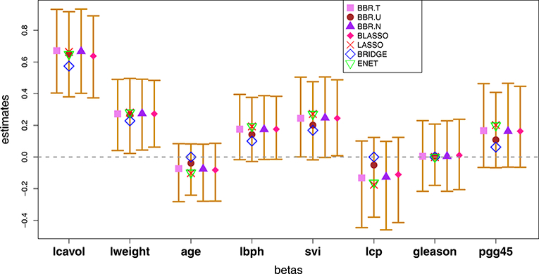
For the prostate data, posterior mean estimates and corresponding 95% equal-tailed credible intervals for Bayesian methods. Overlaid are LASSO, elastic net, and classical bridge estimates based on cross-validation.
Figure 9:
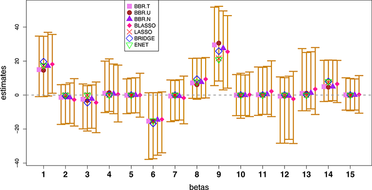
For the pollution data, posterior mean estimates and corresponding 95% equal-tailed credible intervals for Bayesian methods. Overlaid are LASSO, elastic net, and classical bridge estimates based on cross-validation.
6. Computing MAP Estimates
In this section, we provide an EM algorithm to find the approximate posterior mode estimates. It is well known that bridge regularization with 0 < α < 1 leads to a nonconcave optimization problem. To tackle the non-convexity of the penalty function, various approximations have been suggested (Park and Yoon, 2011). One such approximation is the local linear approximation (LLA) proposed by Zou and Li (2008), which can be used to compute the approximate MAP estimates of the coefficients. Treating β as the parameter of interest and∅ = (σ2, λ ) as the ‘missing data’, the complete data log-likelihood based on the LLA approximation is given by
| (10) |
which can be rewritten as
| (11) |
Where, C is a constant w.r.t β, RSS is the residual sum of squares, and are the initial values usually taken as the OLS estimates (Zou and Li, 2008). We initialize the algorithm by starting with a guess of β, σ2, and λ. Then, at each step of the algorithm, we update β by maximizing the expected log conditional posterior distribution. Finally, we replace λ and σ2 in the log posterior (11) by their expected values conditional on the current estimates of β. Following a similar derivation in Sun et al. (2010), the algorithm proceeds as follows:
M-Step:
E-Step:
where RSS(t+1) is the residual sum of squares re-calculated at β (t+1), t = 1, 2, … and is the jth diagonal element of the matrix (XT X)−1. At convergence of the algorithm, we summarize inferences using the latest estimates of β. Unlike the MCMC algorithm described before, this algorithm is likely to shrink some coefficients exactly to zero.
7. Extensions
7.1. Extension to General Models
In this section, we briefly discuss how BBR.U can be extended to several other models beyond linear regression. Let us denote by L(β) the negative log-likelihoodf. Following Wang and Leng (2007), L(β) can be approximated by least squares approximation (LSA) as follows
where is the MLE of β and . Therefore, for a general model, the conditional distribution of y is given by
Thus, we can easily extend our method to several other models by approximating the corresponding likelihood by normal likelihood. Combining the SMU representation of the GG density and the LSA approximation of the general likelihood, the hierarchical presentation of BBR.U (for a fixed α) for general models can be written as
| (12) |
The full conditional distributions are given as
| (13) |
| (14) |
| (15) |
As before, an efficient Gibbs sampler can be easily carried out based on these full conditionals. As noted by one anonymous reviewer, the accuracy of the LSA approximation depends on large sample theory, and it is not clear whether the use of the LSA method is theoretically justified when the sample size is small. As a very preliminary evaluation regarding the potential usefulness of the LSA method, Leng et al. (2014) recently used this approximation for Bayesian adaptive LASSO regression for general models, which showed favorable performance of the MCMC algorithm in moderate to large sample sizes. While their findings are encouraging, further research is definitely needed to better understand the accuracy of the LSA approximation in the context of full posterior sampling. Therefore, caution should be exercised in using the LSA approximation in practice.
7.2. Extension to Group Bridge Regularization
Next we describe how BBR.U can be extended to more general regularization methods such as group bridge (Park and Yoon, 2011) and group LASSO (Yuan and Lin, 2006). Assuming that there is an underlying grouping structure among the predictors, i.e. , where βk is the mk-dimensional vector of coefficients corresponding to group k(k = 1,…, K, ,) and K < p, where K is the number of groups), Park and Yoon (2011) proposed ageneralization of bridge estimator viz. group bridge (which includes group LASSO (Yuan and Lin, 2006) and adaptive group LASSO (Wang and Leng, 2008) as special cases) that results from the following regularization problem
| (16) |
where || βk||2 is the L2 norm of βk, α > 0 is the concavity parameter, and λk > 0, k =1,… , K are the group-specific tuning parameters. Park and Yoon (2011) showed that under certain regularity conditions, the group bridge estimator achieves the ‘oracle group selection’ consistency. For a Bayesian analysis of the group bridge estimator, one may consider thefollowing prior on the coefficients
| (17) |
which belongs to the family of multivariate GG distributions (Gómez-Sánchez-Manzano et al., 2008; Gómez-Villegas et al., 2011). Now, assuming a linear model and using a similar SMU representation of the associated prior (Appendix C in the Supplementary file), the hierarchical representation of the Bayesian group bridge estimator (for a fixed α) can be formulated as follows
| (18) |
The full conditional distributions can be derived as
| (19) |
| (20) |
| (21) |
| (22) |
8. Conclusion and Discussion
We have considered a Bayesian analysis of classical bridge regression based on an SMU representation of the Bayesian bridge prior. We have examined sufficient conditions for the Bayesian bridge posterior consistency under a suitable sparsity assumption on the high-dimensional parameter. We have shown that the proposed method performs as well as or better than existing Bayesian and non-Bayesian methods across a wide range of scenarios, revealing satisfactory performance in both sparse and dense situations. We have further discussed how the proposed method can be easily generalized to several other models, providing a unified framework for modeling a variety of outcomes (e.g. continuous, binary, count, and time-to-event, among others). We have shown that in the absence of an explicit SMN representation of the GG distribution, SMU representation seems to provide important advantages.
We anticipate several statistical and computational refinements that may further improve the performance of the proposed method. While BBR.U considers a single tuning parameter, this may not be optimal in practice (Zou, 2006). Extension to alternative methods that adaptively regularize the coefficients (Leng et al., 2014; Zou, 2006) may improve on this. The theoretical work laid out in this study can be refined further through the investigation of other desired mathematical properties such as posterior contraction (Bhattacharya et al., 2015) and geometric ergodicity (Khare and Hobert, 2013; Pal and Khare, 2014), among others. The unified framework offered by SMU representation makes Bayesian regularization very attractive, opening up possibilities of further investigation in future studies.
Supplementary Material
Figure 2:
Boxplots summarizing the prediction performance of various methods under Model 2.
Figure 5:
Boxplots summarizing prediction performance of various methods under Model 5.
ACKNOWLEDGEMENTS:
We thank the Associate Editor and the two anonymous reviewers for their helpful comments. This work was supported in part by the research computing resources acquired and managed by University of Alabama at Birmingham IT Research Computing. Any opinions, findings, and conclusions or recommendations expressed in this material are those of the authors and do not necessarily reflect the views of the University of Alabama at Birmingham. Himel Mallick was supported in part by the research grants U01 NS041588 and NSF 1158862. Nengjun Yi was supported in part by the research grant NIH 5R01GM069430–08.
References
- Armagan A. Variational bridge regression. Journal of Machine Learning Research W & CP, 5:17–24, 2009. [Google Scholar]
- Armagan A, Dunson DB, Lee J, Bajwa WU, and Strawn N. Posterior consistency in linear models under shrinkage priors. Biometrika, 100(4):1011– 1018, 2013. [Google Scholar]
- Bhattacharya A, Pati D, Pillai NS, and Dunson DB. Dirichlet-laplace priors for optimal shrinkage. Journal of the American Statistical Association, 110(512):1479–1490 [DOI] [PMC free article] [PubMed] [Google Scholar]
- Breheny P and Huang J. Penalized methods for bi-level variable selection. Statistics and its interface, 2(3):369, 2009. [DOI] [PMC free article] [PubMed] [Google Scholar]
- Damien P and Walker SG. Sampling truncated normal, beta and gamma densities. Journal of Computational And Graphical Statistics, 10(2):206–215, 2001. [Google Scholar]
- Devroye Luc. Random variate generation for exponentially and polynomially tilted stable distributions. ACM Transactions on Modeling and Computer Simulation (TOMACS), 19(4):18, 2009. [Google Scholar]
- Frank I and Friedman JH. A statistical view of some chemometrics regression tools (with discussion). Technometrics, 35:109–135, 1993. [Google Scholar]
- Friedman J, Hastie T, and Tibshirani R. Regularization paths for generalized linear models via coordinate descent. Journal of Statistical Software, 33(1):1–22, 2010. [PMC free article] [PubMed] [Google Scholar]
- Gelman A and Rubin DB. Inference from iterative simulation using multiple sequences. Statistical Science, 7(4):457–472, 1992. [Google Scholar]
- Golub Gene H, Heath Michael, and Wahba Grace. Generalized cross-validation as a method for choosing a good ridge parameter. Technometrics, 21(2):215–223, 1979. [Google Scholar]
- Gómez-Sánchez-Manzano E, Gómez-Villegas MA, and Marín JM. Multivariate exponential power distributions as mixtures of normal distributions with bayesian applications. Communications in Statistics—Theory and Methods, 37(6):972–985, 2008. [Google Scholar]
- Gómez-Villegas Miguel A, Gómez-Sánchez-Manzano Eusebio, Maín Paloma, and Navarro Hilario. The effect of non-normality in the power exponential distributions In Modern Mathematical Tools and Techniques in Capturing Complexity, pages 119–129. Springer, 2011. [Google Scholar]
- Hoerl AE and Kennard RW. Ridge regression: biased estimation for nonorthogonal problems. Technometrics, 12:55–67, 1970. [Google Scholar]
- Hyndman Rob J and Koehler Anne B. Another look at measures of forecast accuracy. International Journal of Forecasting, 22(4):679–688, 2006. [Google Scholar]
- Khare Kshitij and Hobert James P. Geometric ergodicity of the bayesian lasso. ElectronicJournal of Statistics, 7:2150–2163 1935–7524, 2013. [Google Scholar]
- Knight K and Fu W. Asymptotics for lasso-type estimators. Annals of Statistics, 28(5): 1356–1378, 2000. [Google Scholar]
- Kyung M, Gill J, Ghosh M, and Casella G. Penalized regression, standard errors, and bayesian lassos. Bayesian Analysis, 5:369–412, 2010. [Google Scholar]
- Leng Chenlei, Tran Minh-Ngoc, and Nott David. Bayesian adaptive lasso. Annals of theInstitute of Statistical Mathematics, 66(2):221–244 [Google Scholar]
- Li Yifang and Ghosh Sujit K. E cient sampling methods for truncated multivariate normal and student-t distributions subject to linear inequality constraints. Journal of Statistical Theory and Practice, 9(4):712–732, 2015. [Google Scholar]
- Mallick Himel. Some Contributions to Bayesian Regularization Methods with Applications toGenetics and Clinical Trials. PhD thesis, University of Alabama at Birmingham, 2015. [Google Scholar]
- Mallick Himel and Yi Nengjun. A new bayesian lasso. Statistics and its interface, 7(4):571,2014. [DOI] [PMC free article] [PubMed] [Google Scholar]
- Mallick Himel and Yi Nengjun. Bayesian group bridge for bi-level variable selection. Computational Statistics and Data Analysis, 110(6):115–133, 2017. [DOI] [PMC free article] [PubMed] [Google Scholar]
- McDonald GC and Schwing RC. Instabilities of regression estimates relating air pollution to mortality. Technometrics, 15(3):463–481, 1973. [Google Scholar]
- Pal Subhadip and Khare Kshitij. Geometric ergodicity for bayesian shrinkage models. Electronic Journal of Statistics, 8(1):604–645 [Google Scholar]
- Park C and Yoon YJ. Bridge regression: adaptivity and group selection. Journal of Statistical Planning and Inference, 141:3506–3519, 2011. [Google Scholar]
- Park T and Casella G. The bayesian lasso. Journal of the American Statistical Association, 103:681–686, 2008. [Google Scholar]
- Phillippe A. Simulation of right and left truncated gamma distributions by mixtures. Statistics and Computing, 7(3):173–181, 1997. [Google Scholar]
- Polson NG, Scott JG, and Windle J. The bayesian bridge. Journal of the Royal Statistical Society, Series B (Methodological), 76(4):713–733, 2014. [Google Scholar]
- Stamey T, Kabalin J, McNeal J, Johnstone I, Frieha F, Redwine E, and Yang N. Prostate specific antigen in the diagnosis and treatment of adenocarcinoma of the prostate ii: Radical prostatectomy treated patients. Journal of Urology, 16:1076–1083, 1989. [DOI] [PubMed] [Google Scholar]
- Sun W, Ibrahim JG, and Zou F. Genomewide multiple-loci mapping in experimental crosses by iterative adaptive penalized regression. Genetics, 185(1):349–359, 2010. [DOI] [PMC free article] [PubMed] [Google Scholar]
- Tibshirani R. Regression shrinkage and selection via the lasso. Journal of the Royal Statistical Society. Series B (Methodological), 58:267–288, 1996. [Google Scholar]
- Wang H and Leng C. Unified lasso estimation by least squares approximation. Journal of the American Statistical Association, 102(479):1039–1048, 2007. [Google Scholar]
- Wang H and Leng C. A note on adaptive group lasso. Computational Statistics & Data Analysis, 52(12):5277–5286, 2008. [Google Scholar]
- West Mike. On scale mixtures of normal distributions. Biometrika, 74(3):646–648, 1987. [Google Scholar]
- Xu Z, Zhang H, Wang Y, Chang X, and Liang Y. L 1/2 regularization. Science China Information Sciences, 53(6):1159–1169, 2010. [Google Scholar]
- Yuan M and Lin N. Model selection and estimation in regression with grouped variables. Journal of the Royal Statistical Society. Series B (Methodological), 68:49–67, 2006. [Google Scholar]
- Zou H. The adaptive lasso and its oracle properties. Journal of the American Statistical Association, 101:1418–1429, 2006. [Google Scholar]
- Zou H and Hastie T. Regularization and variable selection via the elastic net. Journal of the Royal Statistical Society. Series B (Methodological), 67:301–320, 2005. [Google Scholar]
- Zou H and Li R. One-step sparse estimates in nonconcave penalized likelihood models. Annals of Statistics, 36(4):1509, 2008. [DOI] [PMC free article] [PubMed] [Google Scholar]
Associated Data
This section collects any data citations, data availability statements, or supplementary materials included in this article.