Associations between multipollutant day types and select cardiorespiratory outcomes in Columbia, South Carolina, 2002 to 2013

Abstract

Background:

Health studies of air pollution are increasingly aiming to study associations between air pollutant mixtures and health.

Objective:

Estimate associations between observed combinations of ambient air pollutants and select cardiorespiratory outcomes in Columbia, SC during 2002 to 2013.

Methods:

We estimate associations using a two-stage approach. First, we identified a collection of observed pollutant combinations, which we define as multipollutant day types (MDTs), by applying a self-organizing map (SOM) to daily measures of nitrogen dioxide (NO₂), sulfur dioxide (SO₂), ozone (O₃), and particulate matter ≤ 2.5 microns (PM_2.5). Then, overdispersed Poisson time-series models were used to estimate associations between MDTs and each outcome using a ‘clean’ MDT referent and controlling for long-term, seasonal, and day-of-the-week trends and meteorology. Outcomes included daily emergency department visits for asthma and upper respiratory infection (URI), and hospital admissions for congestive heart failure (CHF) and ischemic heart disease (IHD).

Results:

We found that a number of MDTs were significantly and positively associated (point estimates ranged from~2–5%) with cardiorespiratory outcomes in Columbia when compared to days with low pollution. Estimated associations revealed that outcomes for asthma, URIs, and IHD increased 2–4% on warm, dry days experiencing elevated levels of O₃ and PM_2.5. We also found that cooler days with higher NO₂ pollution associated with increased asthma, CHF, and IHD outcomes (2–5%).

Conclusion:

Our analysis continues support for using self-organizing maps to develop multipollutant exposure metrics and further illustrates how such metrics can be applied to explore associations between pertinent pollutant combinations and health.

INTRODUCTION

Outdoor air pollution consists of a mixture of pollutants rather than a single pollutant. Despite this reality, most evidence on the health risks associated with outdoor air pollution, as well as current regulatory strategies to reduce exposure, have largely been based on approaches that define air pollution using a single pollutant such as ozone or particulate matter [1]. While this has generally served us well [2, 3], health scientists, public health professionals, and regulators share a concern that understanding the effects of air pollution can continue to improve if new approaches are further explored [1, 4, 5].

One such area is to begin including multipollutant or mixtures based methodologies into air pollution studies. These directions are motivated by the hope that improved study of this topic will lead to breakthroughs in understanding of environment-disease relationships and increase opportunities for prevention [1, 4, 6]. However, study has proven difficult for many reasons, including problematic designs, highly correlated exposures, complex measurement errors, and differing biological responses, all of which can contribute to making the study of pollutant mixtures a highly complex task [1, 4, 6, 7]. In an effort to overcome such challenges the development of new methods, particularly statistical methods, has become a priority research area in environmental health [1, 4].

In response, several statistical approaches have emerged; these include classic linear regression, classification and prediction, exposure-response surface estimation, variable selection, and variable shrinkage methodologies [8]. Each explores the problem in a unique way, resulting in different benefits, drawbacks and conclusions that can be taken away and thus it has been recommended that investigators choose a method based on the study objectives [8]. For example, a study may seek to identify which pollutants to include in the mix, identify a hidden pattern within the mix, or estimate the health effect of the mix, or all three and thus it should not be unexpected that a number of tools may be required. Thus, to better understand which tools are needed and which questions can be addressed there is an increasing demand for new studies [1, 6, 9].

Here, we present findings from an acute health effects study of air pollution for Columbia, South Carolina (SC) during the years 2002 to 2013. The objective of the study was to assess associations between ambient air pollution mixtures and select cardiorespiratory outcomes. We seek to answer the following research questions:

• What types of day-level pollutant combinations were observed in Columbia, SC and how often did they occur?

• Were certain pollutant combinations more strongly associated with cardiorespiratory outcomes?

We address these objectives using a two-stage approach that involved applying a self-organizing map (SOM) to create a collection of categories we define as multipollutant day types (MDTs) and linking them to specific cardiorespiratory outcomes using a standard time-series regression model [10, 11]. We note that our approach builds upon previous studies of Atlanta that explored development of multipollutant day types for characterizing air quality mixtures and for their application in estimating associations between complex mixtures and asthma morbidity [12, 13]. Here we expand upon previous work by examining associations for a larger number of health outcomes and through application in a new study area.

METHODS

Health Outcome Data

We obtained all emergency department (ED) visits and hospital admissions (HA) for health outcomes in SC defined with primary International Classification of Diseases Ninth Revision (ICD-9) diagnoses of asthma (493, 786.07), upper respiratory infections (URIs: 460–465, 466.0, 477), congestive heart failure (CHF: 428), and ischemic heart disease (IHD: 410–414) from the South Carolina Revenue and Fiscal Affairs Office of Health Statistics. Daily counts of individual events were then summed for all residential ZIP Code Tabulation Areas (ZCTAs) within the Core Based Statistical Area (CBSA) of Columbia, SC (Figure 1) during the years 2002 to 2013.

Figure 1:

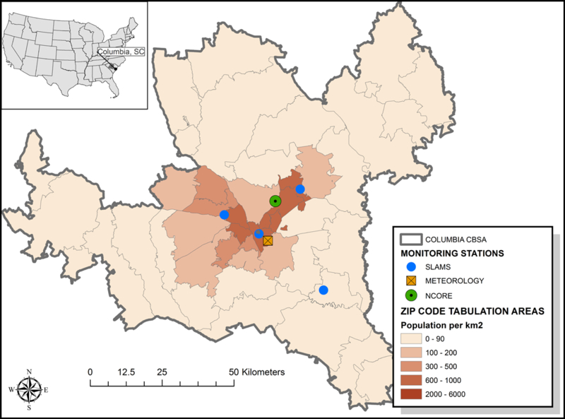
Map of study area.

Environmental Data

Daily exposures were based on stationary air monitoring data obtained for Columbia, SC, from EPA’s State or Local Air Monitoring Stations (SLAMS, n=3) and NCore (n=1) site operated by the South Carolina Department of Health and Environmental Control (Figure 1). Day-level pollutant measures included 1-hr maximum nitrogen dioxide (NO₂) in parts per billion (ppb), 8-hr maximum ozone (O₃) in ppb, 1-hr maximum sulfur dioxide (SO₂) in ppb, and 24-hr average particulate matter < 2.5 microns (PM_2.5) in µg/m³. Daily meteorological conditions were obtained from land surface observations collected at that Columbia Metropolitan Airport ground station (GHCND: USW00013883).

Exposure Assessment

In order to determine the main types of day-level pollutant combinations observed and how often they occurred in our air pollution data we applied an approach known as the self-organizing map (SOM) as it has been shown to be beneficial in other similar studies [10, 12, 13]. In brief, SOM is a statistical learning algorithm that not only discovers subgroups in data with similar attributes but also produces a visualization – the ‘map’ – that spatially organizes group profiles based on the similarity of their attributes [10]. Figure 2 provides a hypothetical example of a ‘map’ produced by SOM. Conceptually, the approach is similar to other classification and clustering techniques (such as k-means, classification and regression trees (CART), Bayesian profile regression) as a group profile is the basic unit of inference for describing patterns observed among the attributes of multiple air pollutants [8, 14, 15]. Here, our aim is to discover subgroups of days that exhibit similar patterns in day-level measures of air pollution: categories which we define as multipollutant day types (MDTs) [12, 13]. As such, we apply SOM as an unsupervised learning tool in order to identify MDTs based on empirically derived patterns without the influence of an outcome variable to predict [16, 17]. This involved the following steps: data preparation; identification of a k* that specifies a suitable number of MDTs to target; profile visualization; and development of a categorical exposure variable.

Figure 2.

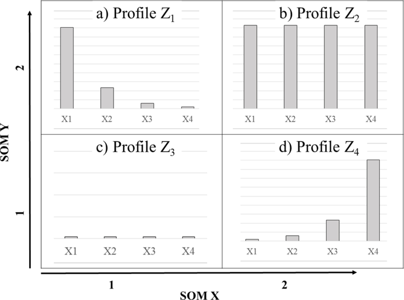
A hypothetical ‘map’ of profiles (Z) produced by a self-organizing map (SOM) set to target four groups, k = 4. Each example profile is illustrated using a bar to reflect the sample mean ($\stackrel{-}{X}$) for component ($X$) during events assigned to profile $Z_k$. SOM coordinates are presented as XY-axes.

To prepare the data, we first selected training days with complete observations (n=3,892) for all pollutants, and then standardized the data measured in different units to have a mean of zero and a standard deviation of one, as we wanted pollutants to have equal influence in profile development [13, 16]. Next, we sought to identify an acceptable k* within the range of k = 2, …, 20 using the following steps: we searched for an obvious k* graphically [16]; 2) we assessed the relationship between exposure classification error and each k; and 3) we assessed the relationship between sample size and each k. Visualization involved applying principal components analysis (PCA) to the pollutant data, and subsequently, plotting the first two components on a biplot to identify if k* could be determined using obvious patterns of correlation among the pollutants that explained the most variation. Next, we examined the exposure classification error as a function of k by assessing the goodness of fit of across each k application. This involved using k MDTs as a categorical predictor, fitting regression models for each pollutant, and examining the resulting adjusted R². Finally, we assessed sample size distributions for MDTs within each k application to get a clearer picture of potential statistical power [12]. We then used this information collectively to determine k*. Profile visualization was achieved by plotting MDT’s on the ‘map’ using mean centered profile bars set to a percentage scale as we desired to compare resulting MDTs to the overall average pollutant conditions. Finally, k* MDTs were used to construct a categorical exposure variable by assigning each day during the study period to its most similar MDT profile and setting the MDT with the lowest pollution values as the referent. All SOM analyses were conducted using functions available in the kohonen and class packages within the R Project for Statistical Computing version 3.4.3 (https://www.r-project.org/). For more detail on SOM implementation in the context of this study please refer to Pearce, et al. [13].

Statistical Analysis

In order to assess if certain pollutant combinations were more strongly associated with cardiorespiratory health, we applied overdispersed Poisson time-series regression models to each outcome separately in order to assess associations with MDTs using a low pollution referent group for an a priori selected exposure lags of 0, 1, 2,and 3 days. Models were fit for each outcome-lag using a dependent variable defined as daily counts of events for the outcome of interest (e.g., asthma ED visit) and MDT assignments for the specified lag period. Each model included covariates to control for confounding by long-term trends and seasonality, day-of-the-week, average temperature, relative humidity, and sea-level pressure. The general structure is:

$$\begin{array}{c}\ln [E(Y_t)]={\beta }_0+\mathit{ns}({\mathit{time}}_t)+\mathit{ns}({\mathit{DOW}}_t)+\mathit{ns}({\mathit{temperature}}_t)+\mathit{ns}({\mathit{relative\; humidity}}_t)\\ +\mathit{ns}({\mathit{sea\; level\; pressure}}_t)+{\displaystyle \sum _{c=1}^{k^{*}-1}}{\delta }_c{{\mathit{MDT}}_c^{(l)}}_t\end{array}$$

where E(Y_t) is the expected number of events for outcome Y on day t, assumed to follow an overdispersed Poisson distribution: β₀ is the model intercept; ns(time_t) is a natural cubic spline for day of study on day t; ns(DOW_t) is a natural cubic spline for day of the week on day t, with 4 df; ns(temperature_t) is a natural cubic spline of the 3-day moving average of temperature on day t and the preceding two days (t − 1, t − 2), with 4 df; ns(relative humidity_t) is a natural cubic spline of the 3-day moving average of mean relative humidity for day ns(sea level pressure_t) is a natural cubic spline of the 3-day moving average of sea level pressure for day t, with 4 df. Finally, our exposure metric $MD{T}_c^{\left(l\right)}{}_t$ is a categorical variable with k^* levels that indicate the assignment of multipollutant day type c on day t for lag model l = 0,1,2,3 [12]. A referent MDT level was specified using the profile that captured days with the lowest overall pollution days.

We reported our risk estimates as rate ratios (RR) along with their 95% confidence intervals (CIs). For comparison, we also fit single pollutant models to determine if our MDTs aligned with more conventional analyses that fit a separate regression model for each pollutant. All analyses were conducted using the stats and splines packages within the R Project for Statistical Computing version 3.4.3 (https://www.r-project.org/).

RESULTS

A total of 2,192,170 cardiorespiratory events occurred among residents of Columbia between January 1, 2002 and December 31, 2013 (Table 1). Of these, 1,700,823 (78%) occurred as ED visits for either asthma or URI and 491,347 (22%) were diagnosed as HA for either CHF or IHD. The average number of daily events for all outcomes was 499, with URIs being the most numerous, followed by IHD, asthma, and CHF, respectively. Generally speaking, events affecting the same bodily system were moderately correlated over time (respiratory r=0.57; cardiovascular r=0.53); however, outcomes across systems did not exhibit much correlation (r < 0.3).

Table 1.

Descriptive statistics for health outcome and environmental data in Columbia, SC from 2002 to 2013.

VARIABLE	ICD-CODE/UNITS	DURATION	CATEGORY	N	MEAN	MEDIAN	MIN	MAX	IQR	STD
Asthma	493, 786.07	24 hr	Emergency Department	288354	66	65	20	152	24	18
Upper Respiratory Infection	460–465, 466.0, 477	24 hr	Emergency Department	1412469	322	306	108	952	152	115
Congestive Heart Failure	428	24 hr	Hospital Admission	184034	42	41	15	78	14	10
Ischemic Heart Disease	410–414	24 hr	Hospital Admission	307313	70	70	20	138	42	24
Nitrogen Dioxide (NO2)	PPB	1 hr	Pollutant	4153	14.8	13.0	0.0	71.0	12.0	8.9
Ozone (O3)	PPB	8 hr	Pollutant	4383	41.1	39.8	1.8	90.7	20.0	14.1
Sulfur Dioxide (SO2)	PPB	1 hr	Pollutant	4265	7.7	5.0	0.0	75.0	9.0	8.1
Particulate Matter ≤ 2.5 (PM2.5)	μg/m3	24 hr	Pollutant	4236	12.2	11.2	1.4	43.3	7.4	5.9
Temperature	C	24 hr	Weather	4383	17.7	18.8	−4.9	33.9	13.7	8.1
Maximum Temperature	C	24 hr	Weather	4383	24.3	25.6	0.0	42.8	12.8	8.3
Minimum Temperature	C	24 hr	Weather	4383	11.9	12.8	−10.6	27.8	16.2	8.9
Wind Speed	m/s	24 hr	Weather	4383	2.5	2.4	0.0	9.2	1.5	1.2
Dewpoint Temperature	C	24 hr	Weather	4383	10.8	12.6	−18.9	24.7	15.3	9.2
Sea Level Pressure	mBAR	24 hr	Weather	4373	1017.6	1017.4	997.2	1040.4	7.3	5.8
Relative Humidity	%	24 hr	Weather	4383	67.9	68.6	22.4	99.3	20.0	13.8

^*Note: Health outcome variables report N as sum of all events and environmental data report N as total number of days measured.

Air pollution data summaries indicated that relatively modest-to-low pollution levels were experienced during our study period (Table 1). The largest day-to-day variability (as measured by the coefficient of variation) was exhibited by SO₂ (105%), followed by NO₂ (60%), PM_2.5 (48%), and O₃ (34%). Correlation among PM_2.5 and O₃ was moderate (r=0.48), but correlation was generally weak between the other pollutants (r<0.3).

Results from the PCA revealed no obvious k* (Figure 3a); however, additional results found that a k* = 6 produced MDTs that explained over 50% of the daily variation in the pollutant data (Figure 3b) and provided sample sizes greater than 5% (Figure 3c). As such, we determined that six MDTs provided a suitable categorization of the days for our study and thus applied a 3X2 SOM to create the final ‘map’ of multipollutant profiles (Figure 4).

Figure 3.

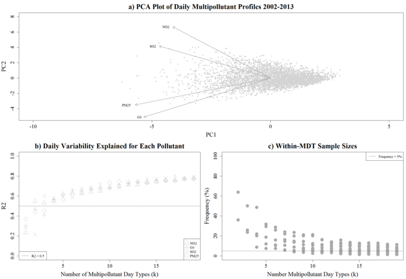
Graphical and statistical evaluation measures used to aid in the selection of the number of multipollutant day types. Panel a) presents a principal components analysis (PCA) projection of our multipollutant data. The grey points represent the scores for daily observations along the first two principal components and the dark arrows indicate the corresponding loading vectors for each pollutant. Panel b) displays the distribution of adjusted R2 values from simple regression models fit to each pollutant as a function of the number of day types. Each pollutant has a unique symbol and the line reflects a threshold of 50%. Panel c) displays the distribution of frequency assignments to each day type. Grey points reflect observed assignments and trend line reflects the expected.

Figure 4.

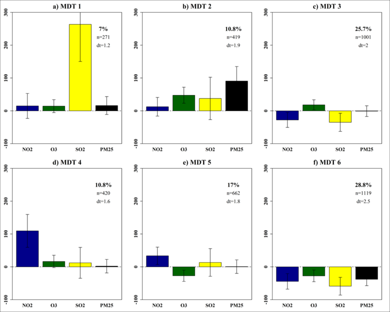
A 3×2 SOM of six multipollutant day types (MDTs) identified in Columbia, SC from January 1, 2002 to December 31, 2013. For each panel, the MDT profile is illustrated using a barplot that reflects the pollutant sample means (error bars reflect one standard deviation) for the group of days assigned to the MDT. Bars have zeroed to the overall (population) mean on presented on a percentage scale. Labels are in at the top of each profile and the relative frequencies (%), within-class sample size (n), and durational time (dt) are presented in the upper right hand corner of each panel.

These results reveal that the most common day type, MDT 6, occurred on 28.8% of days when all pollutant levels were below average (Figure 4f). These ‘clean’ days were well distributed across seasons and experienced broad temperatures, high wind speeds, lower sea-level pressure (SLP), and higher relative humidity suggestive of precipitation (Figure 5). Given these characteristics, we designated MDT 6 as the referent group for subsequent analysis.

Figure 5:

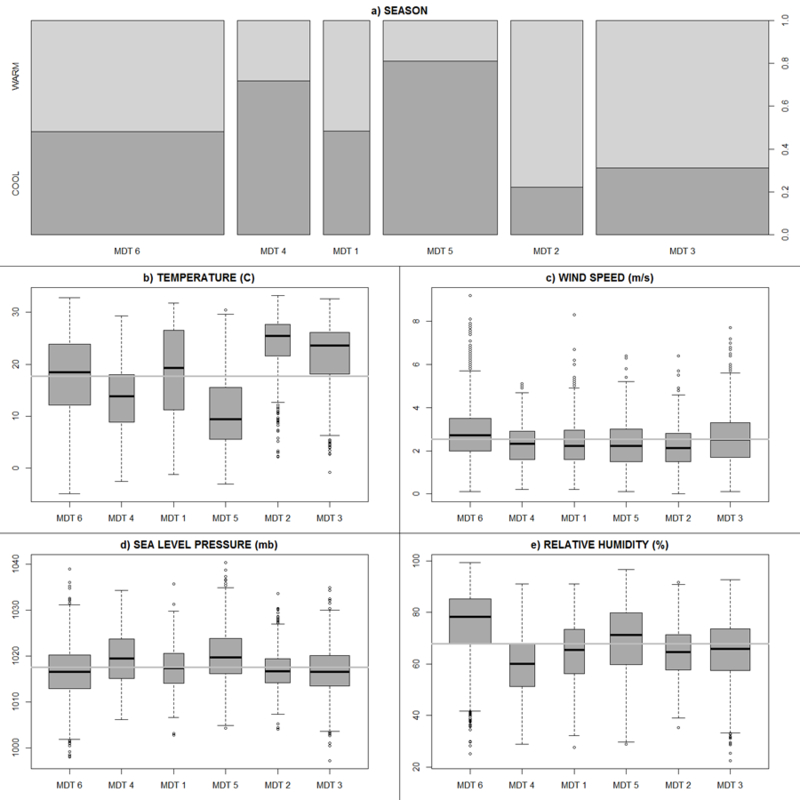
Seasonal frequencies and meteorological summaries for the six multipollutant day types identified in Columbia, SC from January 1, 2002 to December 31, 2013.

The second most common day type, MDT 3, occurred on 25.7% of days and captured conditions when all pollutants were below average with the exception of O₃ (Figure 4c). These days occurred primarily in the warm season and were accompanied with elevated temperatures, moderate winds, and somewhat broad SLP and RH (Figure 5).

The third most common day type, MDT 5, revealed that 17% of days experienced modest increases in NO2 and SO2 and below average O3. These days occurred primarily during the cool season and were accompanied by colder temperatures, low wind speeds, and higher sea-level pressures that suggest periods of atmospheric stability (Figure 5).

Moving to MDT 4 we find cool, stable, dry days (10.8%) dominated by above average NO₂ with above average levels for O₃ and SO₂ (Figure 4d). Moving to MDT 2 we find modestly frequent days (10.8%) that experienced above average levels for all pollutants – particularly O₃ and PM_2.5, and were accompanied by hot, stable, and dry weather. With MDT 1, we find the least frequent profile (7%) capturing days that exhibited relatively high levels of SO₂ accompanied by modest increases all other pollutants (Figure 4a).

Overall, the MDTs capture a broad range of observed multipollutant combinations, with profiles nearer to the bottom right representing more ‘typical’ air quality days dominated by relatively low levels and profiles nearer to the upper left reflecting ‘rare’ events dominated by relative air pollution exposure extremes. Evaluation of daily transitions (dt) suggests profile assignments changed every one to two days with more frequent profiles having stronger persistence (e.g., MDT 6 dt=2.5).

Using MDT 6 as a referent, our statistical analysis identified multiple significant positive associations between MDTs and cardiorespiratory outcomes within a four-day exposure window (Figure 6). Overall, risk ratios (RR) reveal associations of ~2–5% in three outcomes occurred following exposure to several of our MDTs. More specifically, results for asthma reveal significant positive associations with MDT 3 (lag 2 and 3) and MDT 4 (lag 3) and marginally (p-value < 0.1) positive associations with MDT 2 (lag 3) and MDT 5 (lag 3). For URIs, we found significant positive associations with MDT 3 (lag 0, 1, and 2) and marginal positive association with MDT 1 (lag 0), MDT 2 (lag 1, 2), and MDT 4 (lag 3). Marginally positive associations for CHF were shown for MDT 4 (lag 0, 3). For IHD, significant positive associations were identified for MDT 1 (lag 0), MDT 2 (lag 0), MDT 4 (lag 0) and MDT 5 (lags 0) with corresponding marginal associations for MDT 1 and MDT 2 at lag 1. Overall, these findings reveal significant positive associations between days having a variety of multipollutant characteristics and cardiorespiratory outcomes when compared to relatively clean days, in Columbia, SC.

Figure 6.

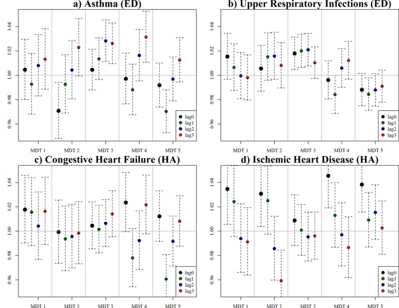
Rate ratios (RR) of health outcomes for days assigned under each multipollutant day type (MDT) as compared to the ‘clean’ air referent group MDT 6.

For comparison, we fitted conventional single-pollutant models and identified significant positive associations between asthma, URIs, CHF, and IHD with overall risk ratios ranging from 1–3% within three days of an interquartile (IQR) increase in air pollution concentrations (Figure 7). For asthma, we found a significant positive association with NO₂ (lag 3), O₃ (lag 2, 3), and PM_2.5 (lag 2, 3) with the largest RR of 1.8% (95% CI: 1.1–2.2%) for O₃ on lag 2. For URIs, we found significant positive associations with O₃ (lags 1, 2, 3 and 3-day moving average (MA)) and PM_2.5 (lags 1, 2, 3 and 3MA) with the largest RR of 2.2% (1.8–4.1%) for a 3-day moving average of O₃. For CHF, we found a significant positive association with NO₂ (lag 0, 3) with the largest RR of 1.9% on lag 0. Finally, for IHD we found a significant positive association for NO₂ (lag 0; 3MA) and PM_2.5 (lag 0) with the largest risk of 3% (2–4%) for a lag 0 of NO₂. Overall, the alignment between multipollutant and single pollutant findings strengthens evidence of an association between ambient air pollution and adverse cardiorespiratory outcomes in Columbia, SC.

Figure 7:

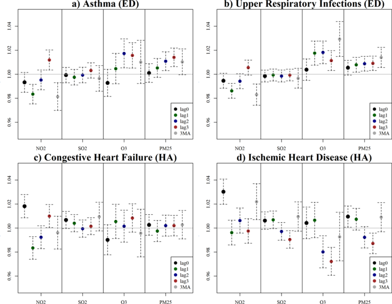
Rate ratios (RR) and 95% confidence intervals for interquartile range (IQR) increases in ambient air pollutant concentration for individual pollutants on the day of event (lag 0), the day before (lag 1), two days before (lag 2), three days before (lag 3) and the three-day moving average (3MA).

DISCUSSION

In this acute health effects study of air pollution in Columbia, SC, we found positive associations between multiple cardiorespiratory outcomes and short-term exposure to air pollution defined using both multipollutant and single pollutant approaches. Multipollutant exposures were defined using multipollutant day types (MDTs) that describe observed day-level combinations among four pollutants during 2002–2013 (Figure 4). Resulting MDTs captured a broad range of daily conditions, ranging from relatively common low pollution days (MDT 6, 29%), to less common days with high levels of multiple pollutants (MDT 2, 11%), to even rarer days dominated by single pollutant extremes (MDT 1, 7%). Subsequent statistical analyses identified clear associations between higher levels of pollution and adverse health when comparisons were made to clean days (MDT 6) (Figure 6). More specifically, we found that occurrence of warmer, dry days with elevated pollution levels (MDTs 2 and 3) were associated with increasing risk for asthma, URIs, and IHD. We also found that cooler days with higher primary source pollution (MDTs 4 and 5) were associated with asthma, CHF, and IHD. Single pollutant extremes (MDT 1) were only found to be significant for IHD. Single pollutant results generally supported these findings (Figure 7). Overall, these findings establish a positive association between air pollution and cardiorespiratory outcomes in our study population which further evidence of health effects of complex environmental mixtures.

As with any study there are limitations of the current work. Broadly, we aimed to identify health associations with complex, multifactorial exposures using a time-series study in which aggregated health outcome and exposure data were compared across a large geographic domain (Figure 1). We chose this approach for its relative ease and low cost; however, common exposure to air pollution, nonspecific outcomes, and estimated risks that tend to be low add to challenges of using this study design to detect subtle health effects (e.g., relative risks often less than 1.10) [6]. Nevertheless, such designs have proven quite useful in studies of air pollution health effects [18] and thus we conducted this study using a careful design that assessed associations based on an exposure metric that maximized contrasts across multiple exposures in the study setting by grouping days under common MDTs. As such, our metric likely suffered from non-differential misclassification of exposure and thus it is highly likely that this led to wider confidence intervals (i.e., bias towards the null) [19]. We attempted to mitigate this issue by making sample size an important aspect of our groupings but note that this was a particularly difficult challenge, as larger sample sizes tend to decrease the number of groupings - a problem that could lead an important mixture being lost under groupings that are too broadly defined. This is an important concern worth noting as exposure characterization errors are inherent with dimension reduction techniques such as the SOM [13].

Another concern is confounding in the context of our multipollutant exposure. We have attempted to use traditional modeling approaches to control for potential confounding (i.e., including covariates for long-term and seasonal trends, day of the week, and weather) but note that -- like other studies seeking to examine the relationship between multipollutant exposures and health effects [20]-- grouping days makes it difficult to confirm that the multipollutant effect is not also encompassing effects of other factors correlated with those day types. An obvious concern here is the weather as certain mixtures may only form under certain meteorological conditions. Finally, we note another challenge for our study is the difficulty in making a direct comparison between our categorically modeled exposure (i.e., multipollutant metric) and our continuously modeled exposure (i.e., single pollutant metric) as different modeling assumptions are made and thus it is difficult to evaluate if one metric more effectively captured risk than the other [20].

Despite these limitations, our study has many strengths that suggest it can support improving understanding of the health risk attributed to air pollution mixtures. First, we improve knowledge of complex exposure to mixtures by conducting a novel exposure assessment that resulted in identification of a collection of observed multipollutant day types (Figure 4). This is an important contribution as it helps understand the nature and magnitude of pollutant combinations observed in our study area and narrows the field for future study.

Secondly, we improve understanding of potential health risk by establishing that certain air pollutant combinations were more strongly associated with adverse events across multiple health outcomes (Figure 6). We note that we did not find a ‘perfect storm’ that was most harmful but rather a range of RRs for day types that suggest adverse health was associated with increasing concentrations for multiple pollutants when compared to low pollution days. This is a finding that agrees well with previous work in Atlanta [12]. In particular, we found that days in the warmer months with pollutant increases (MDT 2 and MDT 3) were more strongly associated with our respiratory outcomes and that cooler days with increasing pollution (MDT 4 and MDT 5) were more strongly associated with our cardiovascular outcomes. Single pollutant findings were similar as they also illustrated outcomes associated positively with several air pollutants. These findings are important as they support a growing body of evidence towards the use of multipollutant exposure profiles to better understand exposure and health effects of complex air pollution mixtures [12, 19–24].

As others have noted, additional research on complex exposure-outcome associations is expected to assist in reducing the burden of air pollution [1, 4, 25]. This could be achieved by integrating multipollutant strategies into primary, secondary, and tertiary prevention of air pollution related disease. For example, primary prevention strategies could be enhanced to include multipollutant day type surveillance, regulation, and warning systems. Secondary prevention could involve enhancing patient education and medical management to reduce exposure on ‘risky’ types of days and tertiary prevention could include improved access to care on such days.

In closing, this work established associations between short-term exposure to types of days defined by their multipollutant profiles and select cardiorespiratory outcomes in a population that generally experience modest-to-low pollution. These are important findings that enhance our understanding of the health risks associated with complex exposures and support hypothesis generation for future study. This was achieved through a novel two-stage frame work that involved, first, applying a self-organizing map (SOM) to identify a manageable number of environmentally relevant pollutant combinations, and second, fitting a standard time-series model to estimate associations with health. We note that we continue to find this SOM-based approach attractive as it is highly flexible and can be broadly applied to future studies seeking to identify relevant types of environmental mixtures and link them with health.

REFERENCES

- 1.Dominici F, Peng RD, Barr CD, and Bell ML, Protecting human health from air pollution: shifting from a single-pollutant to a multi-pollutant approach. Epidemiology (Cambridge, Mass.), 2010. 21(2): p. 187. [DOI] [PMC free article] [PubMed] [Google Scholar]
- 2.Pope CA, Dockery DW, and Schwartz J, Review of epidemiological evidence of health effects of particulate air pollution. Inhalation toxicology, 1995. 7(1): p. 1–18. [Google Scholar]
- 3.Brunekreef B and Holgate ST, Air pollution and health. The Lancet, 2002. 360(9341): p. 1233–1242. [DOI] [PubMed] [Google Scholar]
- 4.Carlin DJ, Rider CV, Woychik R, and Birnbaum LS, Unraveling the health effects of environmental mixtures: an NIEHS priority. Environ Health Perspect, 2013. 121(1): p. A6–A8. [DOI] [PMC free article] [PubMed] [Google Scholar]
- 5.Kelly FJ and Fussell JC, Air pollution and public health: emerging hazards and improved understanding of risk. Environmental geochemistry and health, 2015. 37(4): p. 631–649. [DOI] [PMC free article] [PubMed] [Google Scholar]
- 6.Dockery DW, Epidemiologic study design for investigating respiratory health effects of complex air pollution mixtures. Environmental Health Perspectives, 1993. 101(Suppl 4): p. 187. [DOI] [PMC free article] [PubMed] [Google Scholar]
- 7.Tolbert PE, Klein M, Peel JL, Sarnat SE, and Sarnat JA, Multipollutant modeling issues in a study of ambient air quality and emergency department visits in Atlanta. Journal of Exposure Science and Environmental Epidemiology, 2007. 17(S2): p. S29. [DOI] [PubMed] [Google Scholar]
- 8.Taylor KW, Joubert BR, Braun JM, Dilworth C, Gennings C, Hauser R, Heindel JJ, Rider CV, Webster TF, and Carlin DJ, Statistical approaches for assessing health effects of environmental chemical mixtures in epidemiology: lessons from an innovative workshop. Environmental Health Perspectives, 2016. 124(12): p. A227. [DOI] [PMC free article] [PubMed] [Google Scholar]
- 9.Sexton K and Hattis D, Assessing cumulative health risks from exposure to environmental mixtures—three fundamental questions. Environmental Health Perspectives, 2007. 115(5): p. 825. [DOI] [PMC free article] [PubMed] [Google Scholar]
- 10.Kohonen T, The self-organizing map. Neurocomputing, 1998. 21(1–3): p. 1–6. [Google Scholar]
- 11.Dominici F, Sheppard L, and Clyde M, Health effects of air pollution: a statistical review. International Statistical Review, 2003. 71(2): p. 243–276. [Google Scholar]
- 12.Pearce JL, Waller LA, Mulholland JA, Sarnat SE, Strickland MJ, Chang HH, and Tolbert PE, Exploring associations between multipollutant day types and asthma morbidity: epidemiologic applications of self-organizing map ambient air quality classifications. Environmental Health, 2015. 14(1): p. 55. [DOI] [PMC free article] [PubMed] [Google Scholar]
- 13.Pearce JL, Waller LA, Chang HH, Klein M, Mulholland JA, Sarnat JA, Sarnat SE, Strickland MJ, and Tolbert PE, Using self-organizing maps to develop ambient air quality classifications: a time series example. Environmental Health, 2014. 13(1): p. 56. [DOI] [PMC free article] [PubMed] [Google Scholar]
- 14.Davalos AD, Luben TJ, Herring AH, and Sacks JD, Current approaches used in epidemiologic studies to examine short-term multipollutant air pollution exposures. Annals of epidemiology, 2017. 27(2): p. 145–153. e1. [DOI] [PMC free article] [PubMed] [Google Scholar]
- 15.Oakes M, Baxter L, and Long TC, Evaluating the application of multipollutant exposure metrics in air pollution health studies. Environment international, 2014. 69: p. 90–99. [DOI] [PubMed] [Google Scholar]
- 16.Kaufman L and Rousseeuw PJ, Finding groups in data: an introduction to cluster analysis Vol. 344 2009: John Wiley & Sons. [Google Scholar]
- 17.Friedman J, Hastie T, and Tibshirani R, The elements of statistical learning Vol. 1 2001: Springer series in statistics New York. [Google Scholar]
- 18.Kim K-H, Kabir E, and Kabir S, A review on the human health impact of airborne particulate matter. Environment international, 2015. 74: p. 136–143. [DOI] [PubMed] [Google Scholar]
- 19.Ljungman PL, Wilker EH, Rice MB, Austin E, Schwartz J, Gold DR, Koutrakis P, Benjamin EJ, Vita JA, and Mitchell GF, The impact of multi-pollutant clusters on the association between fine particulate air pollution and microvascular function. Epidemiology (Cambridge, Mass.), 2016. 27(2): p. 194. [DOI] [PMC free article] [PubMed] [Google Scholar]
- 20.Gass K, Klein M, Sarnat SE, Winquist A, Darrow LA, Flanders WD, Chang HH, Mulholland JA, Tolbert PE, and Strickland MJ, Associations between ambient air pollutant mixtures and pediatric asthma emergency department visits in three cities: a classification and regression tree approach. Environmental Health, 2015. 14(1): p. 58. [DOI] [PMC free article] [PubMed] [Google Scholar]
- 21.Austin E, Coull BA, Zanobetti A, and Koutrakis P, A framework to spatially cluster air pollution monitoring sites in US based on the PM2. 5 composition. Environment international, 2013. 59: p. 244–254. [DOI] [PMC free article] [PubMed] [Google Scholar]
- 22.Coker E, Liverani S, Ghosh JK, Jerrett M, Beckerman B, Li A, Ritz B, and Molitor J, Multi-pollutant exposure profiles associated with term low birth weight in Los Angeles County. Environment international, 2016. 91: p. 1–13. [DOI] [PubMed] [Google Scholar]
- 23.Coker E, Liverani S, Su JG, and Molitor J, Multi-pollutant Modeling Through Examination of Susceptible Subpopulations Using Profile Regression. Current environmental health reports, 2018. 5(1): p. 59–69. [DOI] [PubMed] [Google Scholar]
- 24.Keller JP, Drton M, Larson T, Kaufman JD, Sandler DP, and Szpiro AA, Covariate-adaptive clustering of exposures for air pollution epidemiology cohorts. The annals of applied statistics, 2017. 11(1): p. 93. [DOI] [PMC free article] [PubMed] [Google Scholar]
- 25.West JJ, Cohen A, Dentener F, Brunekreef B, Zhu T, Armstrong B, Bell ML, Brauer M, Carmichael G, and Costa DL, What we breathe impacts our health: improving understanding of the link between air pollution and health 2016, ACS Publications. [DOI] [PMC free article] [PubMed] [Google Scholar]