Integration of Sentinel-1 and Sentinel-2 for Classification and LULC Mapping in the Urban Area of Belém, Eastern Brazilian Amazon

Abstract

In tropical regions, such as in the Amazon, the use of optical sensors is limited by high cloud coverage throughout the year. As an alternative, Synthetic Aperture Radar (SAR) products could be used, alone or in combination with optical images, to monitor tropical areas. In this sense, we aimed to select the best Land Use and Land Cover (LULC) classification approach for tropical regions using Sentinel family products. We choose the city of Belém, Brazil, as the study area. Images of close dates from Sentinel-1 (S-1) and Sentinel-2 (S-2) were selected, preprocessed, segmented, and integrated to develop a machine learning LULC classification through a Random Forest (RF) classifier. We also combined textural image analysis (S-1) and vegetation indexes (S-2). A total of six LULC classifications were made. Results showed that the best overall accuracy (OA) was found for the integration of S-1 and S-2 (91.07%) data, followed by S-2 only (89.53%), and S-2 with radiometric indexes (89.45%). The worse result was for S-1 data only (56.01). For our analysis the integration of optical products in the stacking increased de OA in all classifications. However, we suggest the development of more investigations with S-1 products due to its importance for tropical regions.

1. Introduction

Land Use and Land Cover (LULC) data are important inputs for countries to monitor how their soil and land use are being modified over time [1,2]. It is also possible to identify the impacts of increasing urban environments in different ecosystems [3,4,5,6], monitoring protected areas, and the expansion of deforested areas in tropical forests [1,7,8,9].

Remote sensing data and techniques are used as tools for monitoring changes in environmental protection projects reducing in most cases the prices of surveillance. An example is the LULC approach for monitoring Reduced Emissions from Deforestation and Forest Degradation (REDD+) [10,11] and for ecosystem services (ES) modeling and valuation [12,13,14]. For the latter purpose, the LULC mapping has been used to enhance the results found for Costanza et al. [15] that provided global ES values. In that research, the values have been rectified since its first publication [16,17]; the LULC approach provides land classes which allow to estimate ES by unit area, making it possible to extrapolate ES estimates and values for greater areas and biomes around the world by using the benefit transfer method [1,17,18]. Nonetheless, Song [19] highlights the limitation of these values estimations, since LULC satellite-based products have uncertainties related to the data.

From an Earth Observation (EO) perspective, it is desirable to have free and open data access, e.g., Landsat and Sentinel families [20]. These are orbital sensors which, when combined (Landsat-5–8 and the optical sensor of the Sentinel family, the Sentinel-2, hereafter S-2), will provide a 3-day revisit time on the same point on the Earth surface [21,22]. In contrast, these sensors have a medium-quality spatial resolution (30 m for the Landsat and 10 m for the S-2) when compared with other data, such as the Quickbird (0.6 m) and Worldview (0.5 m), but can deliver satisfactory results when the correct methodology is applied [23,24,25].

More recently, the United States (US) started to consider reintroduce prices for the Landsat products acquisition [26]. That is a step backwards when we consider that more than 100,000 published articles were produced since 2008 when US made Landsat products available for free. In contrast, S-2 products are becoming more popular, and despite not having enough data to produce temporal analysis yet, they have a better spatial resolution to develop more precise results [22,27,28,29].

In the perspective of monitoring areas with high cloud coverage, such as tropical regions and estuarine areas, some developments have been reported in using Synthetic Aperture Radar (SAR) products [30,31,32]. To increase SAR usage products for environmental monitoring and security, the European Spatial Agency (ESA) launched the Sentinel-1 (hereafter S-1) in 2014 [33]. Similar to the S-2 products, the S-1 is available for free in the Copernicus platform and covers the entire Earth [34,35].

Recently, processes such as stacking, coregistration, and data fusion of optical with radar products have been applied to improve classification quality and its accuracy. Although radar polarization may be a barrier to identify some features, this product does not have the presence of atmospheric obstacles, such as clouds [11,27,36].

The synergetic use between optical and radar data is a recognized alternative for urban areas studies [37,38,39]. The literature indicates that although the limitations of the microdots in detecting the variety of spectral signatures over the urban environment, such data aggregation contributes to improve the classification accuracy. Also, the importance of radar data has been emphasized in tropical environmental studies [31,40,41,42], once the cloud coverage in these areas is high throughout the year hindering the use of optical images [43,44], and therefore, making radar data an alternative to acquiring imagery during all months of the year in these locations.

Another alternative described in the literature for accuracy enhancement of final classification results is the inclusion of optical indexes of vegetation, soil, water, among others [45,46,47,48]. Indexes included in the data sets allow us to increase the training data range and class statistical possibilities of classification algorithms, thereby raising their efficacy.

Besides choosing suitable products and deciding how to combine different imagery types, the developer of LULC classifications must test different methodologies to select the most accurate for each landscape analyzed [27,36,49]. In this sense, the Machine Learning (ML) algorithms are presented as optimal solutions to supervised classification, where there is no need of ground information measurements of the entire landscape to determine the different classes of LULC for the whole area. Some ML algorithms have been used to classify images with low, medium, or high spatial resolutions [50,51], among them are the Random Forest (RF) [52], Support Vector Machine (SVM) [53], Artificial Neural Networks (ANN) [54], and the k-nearest neighbor (k-NN) [55]. In addition, for the proper selection of satellite imagery, application (or not) of data fusion, and choosing the fittest classification algorithm method, we should also select computer programs that are robust enough to run each of those LULC ML classifications [50].

In this perspective, this study aims to investigate the synergy use between S-1 and S-2 products to identify the suitability for LULC based on ML classification approach. In addition, derivate products such as vegetation and water indexes and SAR textural analysis were applied in the RF classification to finally test all data sets and select the most thematic accurate product for tropical urban environments at regional spatial scale.

2. Satellite Data and Methods

2.1. Study Area

The selected study area is the city of Belém in the Eastern Amazon, Brazil. The city has a total territorial area of 1059.46 km², subdivided into eight administrative districts, all included in this study [56]. The estimated population in 2017 was 1,452,275 residents. According to the Köppen classification, the climate is tropical Afi, with average annual rainfall reaching 2834 mm [57]. The forest fragments of the locality are classified as Terra Firme and Várzea forests, being subtypes of dense Ombrophilous forests [58]. The humid tropical environments in coastal Amazon is described as a complex environment which involves the relationship of flowing rivers with the ocean, different types of natural and anthropized vegetations, and impervious surfaces [59]. Figure 1 shows the study area considered and the coverage of the selected satellite scenes.

Figure 1.

Study area in the municipality of Belém, state of Pará, Brazil *. * Where (A) is the location in the Brazilian territory of the S-1 and S-2 scenes used; (B) shows the relative tracks of the S-1 scenes and S-2 tile used; and (C) is an RGB composition of the S-2 scene where it is illustrated the complexity of the tropical coastal environment chosen (water bodies, different types of vegetation (dense, lowlands, and mangrove), impervious areas, among other ecosystems).

2.2. Data Source and Collection

The products acquisition of both S-1 and S-2 were performed in the Copernicus open access hub platform considering the cloudy coverage of less than 5% for the S-2 product and the date proximity of the S-1 product in relation to the S-2 (one day of difference). The Planet Labs scenes were acquired through a contract of the Environment and Sustainability Secretariat of the state of Pará, Brazil.

2.2.1. Sentinel-1 Images

In order to cover the whole study area, two S-1 images were collected with an S-1 C-band SAR Interferometric Wide Swath (IW) in dual polarization mode (VV + VH) from 21 July 2017. Data characteristics and the main characteristics of S-1 are described in Table 1.

Table 1.

Main attributes from the Synthetic Aperture Radar (SAR) dataset.

S-1	Operation	Since 03/04/2014-current	SAR data	Imaging date	21/07/2017
	Orbit height	693 km		Swath width	250 km
	Inclination	98.18°		Sub-swaths	3
	Wavelength	C-band (3.75–7.5 cm)		Incidence angle range	29.1–46.0°
	Polarization	Dual (VV + VH)		Spatial resolution	5 × 20 m (single look)
	Temporal resolution	Six days		Pixel Spacing	2.3 × 17.4 m

2.2.2. Sentinel-2 Images

One scene of S-2A Level-1C (hereafter, L1C), with radiometric and geometric corrections, was acquired for this study. The S-2A L1C provides the top of atmosphere (TOP) reflectance. The S-2A L1C has a radiometric resolution of 12 bits, a swath width of 290 km, and the wavelength of its bands range from 443 nm to 2190 nm. The spatial resolution of the bands is distributed as (i) four of 10 m, (ii) six of 20 m, and (iii) three of 60 m. The image selected has 0% of cloud cover and is from 20 July 2017. Disregarding the SWIR/Cirrus band, which was used for the atmospheric correction, all bands were used for the classification step.

2.2.3. Planet Imagery

Seventeen high-resolution Planet scenes acquired in 28 July 2017 were used to validate the RF classification. Since early 2017, the sun-synchronous orbit of this satellite has the temporal resolution of one day, making it an excellent instrument for monitoring and data validation [60,61]. The specifications of the Planet mission for the images acquired are described in Table 2.

Table 2.

Main attributes of Planet Labs imagery and the scene selected.

Temporal resolution	Daily
Swath width	24.6 km × 16.4 km
Orbit Altitude (km)	475 (~98° inclination)
Cloud cover of the scenes	0%
Radiometric resolution	12 bits
Operation	Daily imagery since 14/02/2017-current
Imaging date	28/07/2017
Spectral Bands	Wavelength (nm)	Spatial Resolution (m)
Blue	455–515	3
Green	500–590	3
Red	590–670	3
NIR	780–860	3

2.3. Data Analysis

The data processing is presented in the flowchart illustrated in Figure 2 and involves (i) preprocessing and data integration, (ii) product segmentation and RF classification, and (iii) accuracy assessment and validation.

Figure 2.

Process flowchart for Random Forest (RF) classification of Land Use and Land Cover (LULC) classes using S-1 and S-2 integration and validation with Planet Labs imagery.

2.3.1. Preprocessing Data

The preprocessing of the S-2 consisted in the atmospheric correction of the data, made by Sen2Cor algorithm [36,62,63] to obtain surface reflectance. All S-2 spectral bands were resampled to 10-m spectral resolution using the bilinear upsampling method and a mean downsampling method.

As already indicated, two S-1 images were also used, and a slice assemble technique was required to join them. A split of the subswots IW1 and IW2 was applied to reduce the scene size, hence improving the processing time. The application of the orbit file, radiometric correction, thermal noise removal, and deburst was applied as it is a well-consolidated methodology. We opted not to apply a Speckle filter, using Multilooking with a single look (5 m Range looks and 20 m Azimuth looks). Finally, a range-Doppler terrain correction was applied, using the UTM WGS84 projection and the 30 m SRTM, where 10-m resampling was made to fit the integration requirements [27,36,37,64].

2.3.2. Radar Textures and Multispectral Indexes

All of the derived information, for both S-1 and S-2 data, was calculated in the SNAP 6.0 software. For the S-1 product, we derived three Grey-Level Co-occurrence Matrix (GLCM), with a 5 × 5 mobile window size, in all directions based on the variogram method [65]. In general, GLCM estimates the probability of pixel values (within moving windows) co-occurring in a given direction and a certain distance in the image [66]. We computed the mean, variance, and correlation (Table 3). These GLCM statistics were applied for both VV and VH, generating a total of six products to be added in the RF classification [40,46,67]. Moreover, for the S-2 product, we estimated three different normalized radiometric indexes (NDVI-Normalized Difference Vegetation Index, NDWI-Normalized Difference Water Index, and SAVI-Soil-Adjusted Vegetation Index) (Table 3).

Table 3.

Textural analysis and radiometric indexes employed in this research.

S-2 Indexes		References
Index Applied	Equation *
NDVI	$\frac{\mathrm{NIR}-\mathrm{Red}}{\mathrm{NIR}+\mathrm{Red}}$	[68]
NDWI	$\frac{\mathrm{NIR}-\mathrm{MIR}}{\mathrm{NIR}+\mathrm{MIR}}$	[69]
SAVI	$\frac{\mathrm{L}\times (\mathrm{NIR}-\mathrm{Red})}{\mathrm{NIR}+\mathrm{Red}+0.5}$	[70]
S-1 GLCM Textural Measures
Mean	${\displaystyle \sum _{\mathrm{i},\mathrm{j}=0}^{\mathrm{N}-1}}{\mathrm{iP}}_{\mathrm{i},\mathrm{j}}$	[46]
Variance	${\displaystyle \sum _{\mathrm{i},\mathrm{j}=0}^{\mathrm{N}-1}}{\mathrm{iP}}_{\mathrm{i},\mathrm{j}}\left(\mathrm{i}-\mathsf{\mu }\right)²$
Correlation	$\frac{{\sum }_{\mathrm{i},\mathrm{j}=0}^{\mathrm{N}-1}{\mathrm{iP}}_{\mathrm{i},\mathrm{j}}-{\mathsf{\mu }}_{\mathrm{x}}{\mathsf{\mu }}_{\mathrm{y}}}{{\mathsf{\sigma }}_{\mathrm{x}}{\mathsf{\sigma }}_{\mathrm{y}}}$

* Where NIR is the near infrared band, 842 nm for S-2, for NDVI, NDWI, and SAVI; Red is 665 nm for S-2 for NDVI and SAVI; MIR (Medium Infrared) is 2190 nm for S-2, for NDWI; P(i,j) is a normalized gray-tone spatial dependence matrix such that SUM(i,j = 0, N − 1) (P(i,j)) = 1; i and j represent the rows and columns, respectively, for the measures of Mean, Variance and Correlation; μ is the mean, for the Variance textural measure; and N is the number of distinct grey levels in the quantized image; μ_x. μ_y, σ_x, and σ_y are the means and standard deviations of p_x and p_y, respectively, for the correlation textural measure.

2.3.3. Image Stacking and Image Segmentation

For the image stacking of the S-1 and S-2 products it was used the nearest neighbor resampling method. In the tool selected, two products were used, where the pixel values of one product (the slave) were resampled into the geographical raster of the other (the master) [71]. We used the S-1 product as the master and S-2 data as the slave [27,32,37,63,72]. Subsequently, and similarly, the integration was made with S-2 and vegetation and water indexes, S-1 and GLCM textural measures, and the combination of all products generated [46].

To better aggregate pixels with similar values, a segmentation procedure was performed [32,73,74]. This procedure was made using only the collocation of S-1 and S-2 products. For this, a local mutual best fitting region merging criteria was performed and a Baatz & Schape merging cost criteria selected [75,76]. A total of 82,246 segments were produced.

2.3.4. Random Points’ Classification and RF Image Classification

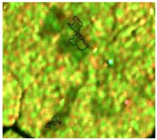
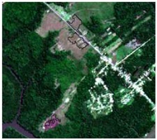
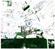
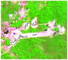
After the segmentation process, all the other steps were developed in GIS software. Basically, 1600 random points were defined to be overlapped by the segmentation polygons, and these were visually interpreted as one of the twelve selected classes. The twelve classes were defined considering the potential attributed by the literature to RF classification algorithm and the S-1 and S-2 synergy, and the particularities of the study area [27,37]. In Table 4 it is possible to identify how the classes were interpreted with colored compositions for S-1 and S-2.

Table 4.

Keys of interpretation to recognize the different LULC with S-1 and S-2 colored compositions.

Classes	Class Code	S-1 (R: VV; G: VH; B: VV/VH) *	S-2 (R: B4; G: B3; B: B2) *	S-2 (R: B12; G: B8; B: B4) *
Agriculture	C1
Airport	C2
Bare Soil	C3
Beach	C4
Built-up	C5
Grassland	C6
Highway	C7
Mining	C8
Primary Vegetation	C9
Urban Vegetation	C10
Water with Sediments	C11
Water without Sediments	C12

* The drawn polygons were the ones produced in the segmentation and classified for each class to perform the LULC classification.

The RF is described in the literature as an ML classification algorithm where the users must choose a minimum of two parameters: (i) the number of trees to grow in the forest (N) and (ii) the depth of those trees (n) [50,52]. We implement this procedure in ArcGIS 10.4 software. The RF classifier in the ArcGIS software is named “Train Random Trees Classifier”. In this classifier, the user must input the following parameters; (i) the satellite image to be classified, (ii) the train sample file (in shapefile format), (iii) the max number of trees (N), (iv) the max tree depth (n), and (v) the max number of samples per class (parameter in which we used the default value of 1000). We also added the segment attributes of Color, Mean, Std, Count, Compactness, and Rectangularity, as they were options in the ArcGIS 10.4 RF algorithm.

To select the number of variables that provide sufficiently low correlation with adequate predictive power, tests were conducted aimed at assessing the best accuracy. All experiments were chosen proportionally with the default values proposed by Forkuor et al. [22]. The best possible scenario, in which the classification was able to run in the ArcGIS 10.4, was with 700 as maximum number of trees (N), 420 as the depth of each tree can grow (n), and 1000 as max number of samples per class; values were applied for all the six classifications made. These numbers were the most significant possible, once the literature suggests that there is no standard value for the number of trees (N) and the number of variables randomly sampled as candidates at each split (n) [50,52].

2.3.5. Accuracy Assessment

As for validation assessments, we carried out a few tests to fully comprehend how the classification was defined and how good was the results found. Firstly, we investigated the mean and standard deviation of the spectral signatures for both S-1 polarizations and for all S-2 bands used for RF classification. With this assessment, we could identify which were the bands that had a greater distance (separation), in the analyzed samples. To evaluate the performance of the attributes and accuracy of the maps produced, we performed statistical approaches based on the separability means of Jeffries–Matusita (JM) and Transformed Divergence (TD), for the two polarizations of S-1 and all bands of the S-2. These coefficients are based on the Bhattacharyya distance statistics and range from 0 to 2, where values greater than 1.8 are quite distinct and values below 1.0 should be disregarded or grouped into a single class [77]. After understanding how the bands statistically separated and how different were their spectral responses, it is also possible to know and how much (algorithm decision making) they contributed to the classification. In this sense, we investigated the bands’ contribution for each LULC classification produced.

As a product of the random trees’ classifier, in ArcGIS 10.4, we analyzed the Producer’s and User’s accuracy (PA and UA, respectively). The PA and UA are prior accuracies (made by 60% of the training samples), which are produced by the trees selected in the model. We analyzed them in the six LULC classification performed.

Finally, by cross-validation performed through the collection and visual interpretation of classes (in Planet’s high spatial resolution images) of 1232 random points, we computed the overall accuracy (OA) and the Kappa coefficient. These are statistics that allow us to analyze and affirm the validity and accuracy of the results. We also ranked these OA and Kappa coefficient values from highest to lowest.

3. Results

The analysis of potentially separable classes through the VV and VH polarizations are presented in Figure 3. The separability found with low values occurs due of a superficial backscatter, highlighting in this case separation in the order of 7 dB, 6 dB, and 9 dB, for airport, beaches, and water with sediment, respectively. On the other hand, we could also identify the occurrence of backscatter double bouncing (built-up areas) and volumetric (primary and secondary vegetation). Because of the identified backscattering, the possibility of class identification through RF increases. However, for the other classes, in which the box plots significantly overlap, the likelihood of variable distinction decreases.

Figure 3.

Backscattering coefficient by LULC class analyzed of VV and VH polarizations of the processed S-1 product *. * The names of the classes respect the class code of the interpretation key as follows. C1 = Agriculture; C2 = Airport; C3 = Bare Soil; C4 = Beach area; C5 = Built-up; C6 = Grassland; C7 = Highway; C8 = Mining; C9 = Primary vegetation; C10 = Urban vegetation; C11 = Water with sediments; C12 = Water without sediments.

For the bands explored in the analysis of separation by the spectral response (surface reflectance) of each class (Figure 4), we could see that some classes tend to get overlaid, once their spectral responses are quite similar in different wavelengths. This was the case for agriculture, grassland, primary vegetation, and urban vegetation, in which the lines generated in the dispersion have close values at different wavelengths. A high separability of classes was noted in the following classes: mining, airport, water with sediments and water without sediments. The classes that present different spectral behaviors from the others tend to perform better classification results since when applying the RF algorithm, it can produce trees and choose the variables for classification with higher precision. The analysis of these backscattering and spectral patterns allows us to provide information for further monitoring of these classes in the study area.

Figure 4.

Wavelengths analysis by LULC class of S-2 bands.

The JM and TD variability results are illustrated in matrix presented in Table 5. For the separability of classes in S-1, we were able to identify only good values (above 1.8) for some airport separability with other classes, for primary vegetation separability with water with sediments and water with sediments with water without sediments. On the other hand, the class separability in for the S-2 bands was significant for different classes, reaching the maximum value for both water categories and primary vegetation. These separability results reassure us that the potential of S-2 to identify a more significant number of classes is significantly better than for the S-1 to do so.

Table 5.

JM and TD * variability results for the similarity of each class. Values in blue represents the variability for S-1 and values in green is for the S-2 *^#.

	C1	C2	C3	C4	C5	C6	C7	C8	C9	C10	C11	C12
C1	-	0.00	0.00	0.00	0.00	0.00	0.00	0.00	0.00	0.00	0.00	0.00
C2	0.00	-	0.00	0.00	0.00	0.00	0.00	0.00	0.00	0.00	0.00	0.00
C3	0.00	1.85	-	0.00	1.73	1.92	1.73	0.00	2.00	1.84	2.00	2.00
C4	0.00	1.52	0.83	-	0.00	0.00	0.00	0.00	0.00	0.00	0.00	0.00
C5	0.00	1.94	0.86	1.50	-	0.00	1.53	0.00	2.00	1.95	2.00	2.00
C6	0.00	1.91	0.51	1.19	0.99	-	1.99	0.00	1.98	1.67	2.00	2.00
C7	0.00	1.91	0.54	1.27	0.10	0.73	-	0.00	2.00	1.92	2.00	2.00
C8	0.00	1.96	0.74	1.12	1.52	0.64	1.33	-	0.00	0.00	0.00	0.00
C9	0.00	2.00	0.92	1.76	1.19	0.28	0.99	1.20	-	1.78	2.00	2.00
C10	0.00	1.98	0.52	1.49	0.46	0.69	0.30	1.29	0.72	-	2.00	2.00
C11	0.00	1.33	1.30	0.43	1.70	1.45	1.55	1.31	1.83	1.79	-	0.18
C12	0.00	1.46	0.98	0.41	1.53	0.94	1.33	0.77	1.36	1.47	1.99	-

* Where the values range from 0 to 2, the higher the value, the better the chance of the class separating into the LULC classification. ^# The classes are represented as follows. C1 = Agriculture; C2 = Airport; C3 = Bare Soil; C4 = Beach area; C5 = Built-up; C6 = Grassland; C7 = Highway; C8 = Mining; C9 = Primary vegetation; C10 = Urban vegetation; C11 = Water with sediments; C12 = Water without sediments.

In Figure 5 it is illustrated the six LULC classification produced.

Figure 5.

LULC classification maps produced by RFs *^#. * Where (A) is for S-1 only, (B) is S-2 only, (C) is S-1 with textures, (D) is S-2 with indexes, (E) is S-1 with S-2, and (F) is for all bands. ^# The classes are represented as follows. C1 = Agriculture; C2 = Airport; C3 = Bare Soil; C4 = Beach area; C5 = Built-up; C6 = Grassland; C7 = Highway; C8 = Mining; C9 = Primary vegetation; C10 = Urban vegetation; C11 = Water with sediments; C12 = Water without sediments.

The contribution of each band for the six RF classifications produced is described in Figure 6A–F. Band 12 of the S-2 product (SWIR band) was the only band that repeats, as the most significant contributor for the RF classification made (see Figure 6B,E), this band is the main contributor for the classifications of S-2 only and the integration of S-1 with S-2. Thus, in all the classifications that contain the S-2 band, some of its bands were identified as one of the most significant contributors to the classification. Therefore, for the classification with all products, the red band of S-2 had the highest contribution (0.0641), for S-1, together with S-2, and for the S-2 only, it was SWIR band 12 of S-2 (0.1 and 0.1067, respectively), and for S-2 and indexes it was the SWIR band 11 (0.084). On the other hand, for the classifications that only consider the SAR products, it was shown that the largest contribution was from S-1 VV (0.6307), and for S-1 and its textures, it was the S-1 VH GLCM Mean (0.1434).

Figure 6.

Bands contribution for RF classification *. * Where (A) is the band’s contribution for the S-1 only, (B) is for S-2 only, (C) is S-1 with textures, (D) is for S-2 with indexes, (E) is S-1 with S-2, and (F) is all bands.

The PA and UA results are presented in Table 6. The optical integration with radar and the optical only classifiers stands out with generally better results of PA. The worst results were found for classifiers without the S-2, being S-1 only and S-1 with GLCM secondary products. The UA followed a similar trend. The worst result by class was found for the agriculture and mining classes in the classifier that used radar and its textures, where the results for both PA and UA were equal to 0%. However, the mining class achieved 100% in PA for all classifiers that had S-2 bands. S-2 only, S-2 with its indexes, and the integration of S-1 with S-2 had more than one PA equal to 100%; Agriculture (C1) and mining (C8) were repeated in all these classifications, for the integration of S-1 and S-2, the Airport (C2) class also had PA equals to 100%. The only UA with 100% was for the identification of beaches in the classification S-2 with indexes.

Table 6.

PA and UA for each class in the different types of RF classifications produced *.

Class Code	S-1 Only		S-2 Only		S-1 with Textures		S-2 with Indexes		S-1 with S-2		All Bands
	PA (%)	UA (%)	PA (%)	UA (%)	PA (%)	UA (%)	PA (%)	UA (%)	PA (%)	UA (%)	PA (%)	UA (%)
C1	50.0	7.7	100.0	18.2	0.0	0.0	100.0	20.0	100.0	20.0	50.0	20.0
C2	60.0	16.7	80.0	66.7	40.0	25.0	80.0	80.0	100.0	50.0	80.0	57.1
C3	31.2	23.8	56.3	64.3	25.0	21.1	56.3	69.2	65.6	75.0	46.9	48.4
C4	40.0	21.1	70.0	77.8	80.0	47.1	80.0	100.0	80.0	88.9	40.0	66.7
C5	41.8	42.2	75.5	85.1	53.1	51.5	79.6	86.7	80.6	94.1	71.4	88.6
C6	27.6	10.3	58.6	60.7	41.4	16.2	51.7	55.6	58.6	63.0	55.2	48.5
C7	12.1	9.3	75.8	59.5	15.2	11.9	78.8	59.1	78.8	70.3	69.7	46.0
C8	20.0	4.0	100.0	55.6	0.0	0.0	100.0	50.0	100.0	50.0	100.0	62.5
C9	46.9	65.7	89.2	94.6	60.7	74.3	88.8	94.3	90.3	94.0	88.8	93.1
C10	16.7	18.1	68.6	64.2	18.6	21.6	66.7	62.4	73.5	70.8	60.8	60.2
C11	41.4	8.6	93.1	81.8	48.3	9.4	93.1	77.1	93.1	75.0	79.3	67.7
C12	75.3	98.5	99.5	99.7	77.2	98.7	99.2	99.7	99.5	99.7	99.0	98.7

* The classes are represented as follows. C1 = Agriculture; C2 = Airport; C3 = Bare Soil; C4 = Beach area; C5 = Built-up; C6 = Grassland; C7 = Highway; C8 = Mining; C9 = Primary vegetation; C10 = Urban vegetation; C11 = Water without sediments; C12 = Water with sediments.

Table 7 illustrates the OA and the Kappa coefficients found in this research. It is possible to understand that the integration of the S-1 and S-2 products resulted in a more precise product (91.07% of OA and 0.8709 of Kappa) and, as expected, the S-1 product alone had the worst result of all the analyses (56.01% of OA and 0.4194 of Kappa). The inclusion of textures in the S-1 products increased the results of the RF classification (61.61% OA and 0.4870 of Kappa), on the other hand, the inclusion of vegetation and water indexes in the S-2 product reduced its OA (89.45%) and Kappa coefficient (0.8476) when compared with the S-2 alone (89.53% of OA and 0.8487 for the Kappa coefficient). The integration of all the products analyzed produced the worst result among all the data combination that have S-2 products involved (87.09% OA and 0.8132 of Kappa coefficient). However, the results of OA and Kappa coefficient for the four best classifications were similar.

Table 7.

OA and Kappa coefficient for each classifier ranked in order of accuracy.

Data Combination	Overall Accuracy (%)	Kappa Coefficient	Rank
S-1 with S-2	91.07	0.8709	1
S-2 Only	89.53	0.8487	2
S-2 with Indexes	89.45	0.8476	3
All	87.09	0.8132	4
S-1 with Textures	61.61	0.4870	5
S-1 Only	56.01	0.4194	6

4. Discussion

Among the ML methods described in the literature [50], SVM and RF stand out for their good classification accuracy. These methods usually have good results when compared with similar methods such as k-NN, or more sophisticated ones, such as ANN and Object Based Image Analysis (OBIA) methods [27,36,49]. Since these two types of ML algorithms are the most outstanding, we analyzed the discussion considering some papers that used both algorithms.

We verified that the application of optical radiometric indexes and radar textures is widely accepted as mean to improve ML classification [11,27,36,46,63,78]. However, our OA result, when considering all bands in the classification, was lower than for S-1 and S-2, S-2 only, and S-2 with indexes. These results show that the insertion of the data derived from the optical image did not have a significant impact on the final classification, whereas the SAR product data, which improved the classification when considering S-1 only, contributed to the classification, but not enough to raise OA when all bands were considered. Some authors argue that major classification enhancements occur only when we insert primary data into the dataset, such as SRTM [63,64,79].

The lowest OA values found were for S-1 products; this is in agreement with what is found in the literature [27,36,40,46,80]. SAR products, while having the advantage of penetrating the clouds and always giving views consistent with the Earth’s surface, fail when forced to distinct a vast amount of features (classes) [80,81]. In our study, this is noticeable in Table 5, in which JM and TD values were lower than 1.8 in almost all categories, and this can be seen in local studies on the Brazilian Amazon coast, even using radar images with better quality than those of S-1 [82,83]. Discrimination of a large number of classes on the radar is possible only through the application of advanced techniques, such as SAR polarimetry [84].

Maschler et al. [85], in an application of the RF classifier with high spatial resolution data of 0.4 m (Hyspex VNIR 1600 airborne data), obtained excellent separability of the classes in the electromagnetic spectrum. From this good separability, they were also able to produce an excellent OA of 91.7%. This separability and these good results can be identified in our study too. The possibility of separating the classes from the insertion of the training and validation samples is fundamental for the satisfactory production of the results for LULC classification.

Among the authors who applied several ML methods (RF, SVM, and k-NN), Clerici et al. [36] consider the data fusion of S-1 and S-2 products. They also applied radiometric vegetation indexes (NDVI, Sentinel-2 Red-Edge Position index (S2REP), Green Normalized Difference Vegetation Index (GNDVI), and Modified SAVI) and textural analysis of the S-1, in order to interpret their contributions to the supervised classification accuracy. Six classes were tested after segmentation to have similar pixel values. Their results were considerably worse than ours. In their image stacking, they found an OA of 55.50% and a Kappa coefficient of 0.49. The isolated results of S-1 and S-2 were also worse than our integration. They suggest SVM for their study area because it presents better accuracy results.

Whyte et al. [27] applied RF and SVM algorithms for LULC classification in the synergy of S-1 and S-2. These authors used the eCognition image processing software to produce segments and the ArcGIS 10.3 for RF and SVM classifications. They applied derivatives from both S-1 and S-2 to test the data combination for LULC. They selected 15 classes and found better results when using all products (S-1, S-2, and their derivatives) using the RF algorithm. The OA was 83.3% and the Kappa coefficient was 0.72. However, all the scenarios of synergy appeared to have higher results than using optical data only. This study contrast to what we found, once our results with derivatives were worse in almost all circumstances, except in S-1 and GLCM stacking.

Zhang & Xu [49] also applied the fusion test of optical images and radar for multiple classifiers (RF, SVM, ANN, and Maximum Likelihood). Optical images of Landsat TM and SPOT 5 were used, while SAR images were of ENVISAT ASAR/TSX. The authors could interpret that the best values were found for the RF and SVM classifications, while the fusion of optical and SAR data contributed to the improvement of the classification, increasing the accuracy by 10%.

Deus [46] used the synergy of ALOS/PALSAR L band and Landsat 5 TM and applied several vegetation indexes and SAR textural analysis. The author applied the SVM algorithm in order to obtain five LULC classes. Their highest OA was 95% when only the features with the best performance in the classification were combined, including both PALSAR and TM bands and their derivatives.

Jhonnerie et al. [86] and Pavanelli et al. [40] also used ALOS/PALSAR and the Landsat family. They considered LULC classes 8 and 17, respectively. Both studies applied the RF algorithm. While the first authors used the ERDAS image application for RF classification, the second authors used the R software for their image classification. They applied vegetation indexes and GLCM textural analysis. For the RF classification, both authors found their highest OA and Kappa coefficient results for the hybrid model, 81.1% and 0.760 [86] and 82.96% and 0.81 [40].

Erinjery et al. [11] also used the synergy between S-1 and S-2, and their derivatives to compare results from two ML, including Maximum Likelihood and RF. The total number of classes was seven. For the RF classification, an OA of 83.5% and a Kappa coefficient of 0.79 were found. They state the inclusion of SAR data and textural features for RF classification as a tool to improve the classification accuracy. Similarly to our study, they found an OA lower than 50% when using only the S-1 product.

Shao et al. [78] integrated the S-1 SAR imagery with the GaoFan optical data to apply a RF classification algorithm in six different LULC classes. They also produce SAR GLCM textures and vegetation indexes. Their best result was obtained considering all the features stacked. An OA of 95.33% and a Kappa coefficient of 0.91 was obtained. The use of S-1 only had the worst result, with an OA of 68.80% and a Kappa coefficient of 0.35.

Haas & Ban [37], in a data fusion analysis of S-1 and S-2, applied the SVM classification method. Considering 14 classes, they found an OA of 79.81% and a Kappa coefficient of 0.78. The authors suggested the postclassification analysis to improve its accuracy once their final objective was to have area values to apply the benefits transfer method of Burkhard et al. [17] to environmentally evaluate the urban ecosystem services of an area. The number of classes was similar to our study, and it was possible to check that the accuracy was superior.

In regional studies [2], and for global applications [87,88] of RF classification, the results found of OA were below those of ours. Their OA results were 75.17% [88], 63% for South America using RF [87], and 76.64% for Amazon LULC classification [2]. All these studies used satellite data with a temporal resolution of 16 days and a spatial resolution of 30 m. In contrast, we found results with a revisit time of five days for optical and six days for SAR, and with a greater spatial resolution (10 m). Also, we produced a dataset with more classes (12) against six [87] and seven [88] classes found for global studies.

5. Conclusions

In this work, the best result found was in the integration of S-1 and S-2 products. In general, integrating the vegetation and water indexes and SAR textural features made the OA and kappa coefficient decrease. The worse result was found for the S-1 only classification. The results encountered agreed in its most part with the literature. For our better classifications, the OA results were significantly greater than what is found in the literature for global and Amazon applications of RF classification.

In both the PA and UA scenarios and the Kappa statistic scenario it can be stated that the integration of S-1 and S-2 presented better results in the implemented ML technique. However, if on the one hand the GLCM increased the SAR product accuracy, on the other hand, the inclusion of vegetation and water indexes decreased the optical accuracy, when compared with the single use of S-1 and S-2, respectively. Lastly, the results found for the integration of all products were worse than the ones observed for the combination of S-1 and S-2 only.

Depending on the final aim of the LULC classification, it could be relevant to make a postclassification analysis because many spectral responses resemble each other and can confuse the ML process. However, in the best scenario produced, the accuracy found was satisfactory for several types of analysis. Furthermore, it is possible to use the data integration of S-1 and S-2 to LULC cover classification in tropical regions. It is noteworthy that few studies with similar methodology were found in the literature for the southern hemisphere.

In this sense, the research findings can contribute to current knowledge on urban land classification since methodology applied produces more accurate local data. Furthermore, the present results were obtained by using a smaller revisit period and a higher number of land classes than previous global studies which considered our study area. Future work must be done with S-1 and its variables; once in tropical regions it is difficult to have long terms of optical data available. Finally, we encourage the synergetic use of S-1 and S-2 for LULC classification, considering the availability on near date.

Author Contributions

Conceptualization, P.A.T., N.E.S.B., and U.S.G.; Data curation, P.A.T.; Formal Analysis, P.A.T., N.E.S.B., U.S.G., and A.C.T.; Funding Acquisition, N.E.S.B. and A.C.T.; Investigation, P.A.T., N.E.S.B., U.S.G., and A.C.T.; Methodology, P.A.T. and U.S.G.; Project Administration, N.E.S.B.; Resources, P.A.T., N.E.S.B., U.S.G., and A.C.T.; Software, P.A.T. and U.S.G.; Supervision, N.E.S.B., U.S.G., and A.C.T.; Validation, P.A.T. and U.S.G.; Visualization, P.A.T., N.E.S.B., U.S.G., and A.C.T.; Writing—Original Draft, P.A.T. and N.E.S.B.; Writing—Review & Editing, P.A.T., N.E.S.B., U.S.G., and A.C.T.

Funding

This research was funded by CAPES—Coordenação de Aperfeiçoamento de Pessoal de Nível grant number 1681775.

Conflicts of Interest

The authors declare no conflict of interest.

References

- 1.Sannigrahi S., Bhatt S., Rahmat S., Paul S.K., Sen S. Estimating global ecosystem service values and its response to land surface dynamics during 1995–2015. J. Environ. Manag. 2018;223:115–131. doi: 10.1016/j.jenvman.2018.05.091. [DOI] [PubMed] [Google Scholar]
- 2.De Almeida C.A., Coutinho A.C., Esquerdo J.C.D.M., Adami M., Venturieri A., Diniz C.G., Dessay N., Durieux L., Gomes A.R. High spatial resolution land use and land cover mapping of the Brazilian Legal Amazon in 2008 using Landsat-5/TM and MODIS data. Acta Amaz. 2016;46:291–302. doi: 10.1590/1809-4392201505504. [DOI] [Google Scholar]
- 3.Wang S., Ma Q., Ding H., Liang H. Detection of urban expansion and land surface temperature change using multi-temporal landsat images. Resour. Conserv. Recycl. 2018;128:526–534. doi: 10.1016/j.resconrec.2016.05.011. [DOI] [Google Scholar]
- 4.Duan J., Wang Y., Fan C., Xia B., de Groot R. Perception of Urban Environmental Risks and the Effects of Urban Green Infrastructures (UGIs) on Human Well-being in Four Public Green Spaces of Guangzhou, China. Environ. Manag. 2018;62:500–517. doi: 10.1007/s00267-018-1068-8. [DOI] [PubMed] [Google Scholar]
- 5.Sahani S., Raghavaswamy V. Analyzing urban landscape with City Biodiversity Index for sustainable urban growth. Environ. Monit. Assess. 2018;190 doi: 10.1007/s10661-018-6854-5. [DOI] [PubMed] [Google Scholar]
- 6.Rimal B., Zhang L., Keshtkar H., Wang N., Lin Y. Monitoring and Modeling of Spatiotemporal Urban Expansion and Land-Use/Land-Cover Change Using Integrated Markov Chain Cellular Automata Model. ISPRS Int. J. Geo-Infor. 2017;6:288. doi: 10.3390/ijgi6090288. [DOI] [Google Scholar]
- 7.Mukul S.A., Sohel M.S.I., Herbohn J., Inostroza L., König H. Integrating ecosystem services supply potential from future land-use scenarios in protected area management: A Bangladesh case study. Ecosyst. Serv. 2017;26:355–364. doi: 10.1016/j.ecoser.2017.04.001. [DOI] [Google Scholar]
- 8.Shaharum N.S.N., Shafri H.Z.M., Gambo J., Abidin F.A.Z. Mapping of Krau Wildlife Reserve (KWR) protected area using Landsat 8 and supervised classification algorithms. Remote Sens. Appl. Soc. Environ. 2018;10:24–35. doi: 10.1016/j.rsase.2018.01.002. [DOI] [Google Scholar]
- 9.Adhikari A., Hansen A.J. Land use change and habitat fragmentation of wildland ecosystems of the North Central United States. Landsc. Urban Plan. 2018;177:196–216. doi: 10.1016/j.landurbplan.2018.04.014. [DOI] [Google Scholar]
- 10.Sirro L., Häme T., Rauste Y., Kilpi J., Hämäläinen J., Gunia K., de Jong B., Pellat F.P. Potential of different optical and SAR data in forest and land cover classification to support REDD+ MRV. Remote Sens. 2018;10:942. doi: 10.3390/rs10060942. [DOI] [Google Scholar]
- 11.Erinjery J.J., Singh M., Kent R. Mapping and assessment of vegetation types in the tropical rainforests of the Western Ghats using multispectral Sentinel-2 and SAR Sentinel-1 satellite imagery. Remote Sens. Environ. 2018;216:345–354. doi: 10.1016/j.rse.2018.07.006. [DOI] [Google Scholar]
- 12.Kwok R. Ecology’s remote-sensing revolution. Nature. 2018;556:137–138. doi: 10.1038/d41586-018-03924-9. [DOI] [PubMed] [Google Scholar]
- 13.Paul C.K., Mascarenhas A.C. Remote Sensing in Development. Science. 1981;214:139–145. doi: 10.1126/science.214.4517.139. [DOI] [PubMed] [Google Scholar]
- 14.Pettorelli N., Laurance W.F., O’Brien T.G., Wegmann M., Nagendra H., Turner W. Satellite remote sensing for applied ecologists: Opportunities and challenges. J. Appl. Ecol. 2014;51:839–848. doi: 10.1111/1365-2664.12261. [DOI] [Google Scholar]
- 15.Costanza R., Arge R., De Groot R., Farber S., Grasso M., Hannon B., Limburg K., Naeem S., O’Neil R.V., Paruelo J., et al. The Value of the World’s Ecosystem Services and Natural Capital. Nature. 1997;387:253–260. doi: 10.1038/387253a0. [DOI] [Google Scholar]
- 16.Costanza R., de Groot R., Braat L., Kubiszewski I., Fioramonti L., Sutton P., Farber S., Grasso M. Twenty years of ecosystem services: How far have we come and how far do we still need to go? Ecosyst. Serv. 2017;28:1–16. doi: 10.1016/j.ecoser.2017.09.008. [DOI] [Google Scholar]
- 17.Burkhard B., Kroll F., Nedkov S., Müller F. Mapping ecosystem service supply, demand and budgets. Ecol. Indic. 2012;21:17–29. doi: 10.1016/j.ecolind.2011.06.019. [DOI] [Google Scholar]
- 18.Lyu R., Zhang J., Xu M. Integrating ecosystem services evaluation and landscape pattern analysis into urban planning based on scenario prediction and regression model. Chin. J. Popul. Resour. Environ. 2018:1–15. doi: 10.1080/10042857.2018.1491201. [DOI] [Google Scholar]
- 19.Song X.P. Global Estimates of Ecosystem Service Value and Change: Taking into Account Uncertainties in Satellite-based Land Cover Data. Ecol. Econ. 2018;143:227–235. doi: 10.1016/j.ecolecon.2017.07.019. [DOI] [Google Scholar]
- 20.Poursanidis D., Chrysoulakis N. Remote Sensing Applications: Society and Environment Remote Sensing, natural hazards and the contribution of ESA Sentinels missions. Remote Sens. Appl. Soc. Environ. 2017;6:25–38. doi: 10.1016/j.rsase.2017.02.001. [DOI] [Google Scholar]
- 21.Li J., Roy D.P. A Global Analysis of Sentinel-2A, Sentinel-2B and Landsat-8 Data Revisit Intervals and Implications for Terrestrial Monitoring. Remote Sens. 2017;9:902. doi: 10.3390/rs9090902. [DOI] [Google Scholar]
- 22.Forkuor G., Dimobe K., Serme I., Tondoh J.E. Landsat-8 vs. Sentinel-2: Examining the added value of sentinel-2’s red-edge bands to land-use and land-cover mapping in Burkina Faso. GISci. Remote Sens. 2018;55:331–354. doi: 10.1080/15481603.2017.1370169. [DOI] [Google Scholar]
- 23.Chen A., Yao X.A., Sun R., Chen L. Effect of urban green patterns on surface urban cool islands and its seasonal variations. Urban For. Urban Green. 2014;13:646–654. doi: 10.1016/j.ufug.2014.07.006. [DOI] [Google Scholar]
- 24.Van de Voorde T. Spatially explicit urban green indicators for characterizing vegetation cover and public green space proximity: A case study on Brussels, Belgium. Int. J. Digit. Earth. 2016;10:798–813. doi: 10.1080/17538947.2016.1252434. [DOI] [Google Scholar]
- 25.Wang H.-F., Qureshi S., Qureshi B.A., Qiu J.-X., Friedman C.R., Breuste J., Wang X.-K. A multivariate analysis integrating ecological, socioeconomic and physical characteristics to investigate urban forest cover and plant diversity in Beijing, China. Ecol. Indic. 2016;60:921–929. doi: 10.1016/j.ecolind.2015.08.015. [DOI] [Google Scholar]
- 26.Popkin G. US government considers charging for popular Earth-observing data. Nature. 2018;556:417–418. doi: 10.1038/d41586-018-04874-y. [DOI] [PubMed] [Google Scholar]
- 27.Whyte A., Ferentinos K.P., Petropoulos G.P. A new synergistic approach for monitoring wetlands using Sentinels-1 and 2 data with object-based machine learning algorithms. Environ. Model. Softw. 2018;104:40–54. doi: 10.1016/j.envsoft.2018.01.023. [DOI] [Google Scholar]
- 28.Rußwurm M., Körner M. Multi-Temporal Land Cover Classification with Sequential Recurrent Encoders. ISPRS Int. J. Geo-Infor. 2018;7:129. doi: 10.3390/ijgi7040129. [DOI] [Google Scholar]
- 29.Szostak M., Hawryło P., Piela D. Using of Sentinel-2 images for automation of the forest succession detection. Eur. J. Remote Sens. 2018;51:142–149. doi: 10.1080/22797254.2017.1412272. [DOI] [Google Scholar]
- 30.Pereira L.O., Freitas C.C., SantaAnna S.J.S., Reis M.S. Evaluation of Optical and Radar Images Integration Methods for LULC Classification in Amazon Region. IEEE J. Sel. Top. Appl. Earth Obs. Remote Sens. 2018:1–13. doi: 10.1109/JSTARS.2018.2853647. [DOI] [Google Scholar]
- 31.Reiche J., Lucas R., Mitchell A.L., Verbesselt J., Hoekman D.H., Haarpaintner J., Kellndorfer J.M., Rosenqvist A., Lehmann E.A., Woodcock C.E., et al. Combining satellite data for better tropical forest monitoring. Nat. Clim. Chang. 2016;6:120–122. doi: 10.1038/nclimate2919. [DOI] [Google Scholar]
- 32.Joshi N., Baumann M., Ehammer A., Fensholt R., Grogan K., Hostert P., Jepsen M.R., Kuemmerle T., Meyfroidt P., Mitchard E.T.A., et al. A review of the application of optical and radar remote sensing data fusion to land use mapping and monitoring. Remote Sens. 2016;8:70. doi: 10.3390/rs8010070. [DOI] [Google Scholar]
- 33.Torres R., Snoeij P., Geudtner D., Bibby D., Davidson M., Attema E., Potin P., Rommen B.Ö., Floury N., Brown M., et al. GMES Sentinel-1 mission. Remote Sens. Environ. 2012;120:9–24. doi: 10.1016/j.rse.2011.05.028. [DOI] [Google Scholar]
- 34.Raspini F., Bianchini S., Ciampalini A., Del Soldato M., Solari L., Novali F., Del Conte S., Rucci A., Ferretti A., Casagli N. Continuous, semi-automatic monitoring of ground deformation using Sentinel-1 satellites. Sci. Rep. 2018;8:1–11. doi: 10.1038/s41598-018-25369-w. [DOI] [PMC free article] [PubMed] [Google Scholar]
- 35.Nagler T., Rott H., Hetzenecker M., Wuite J., Potin P. The Sentinel-1 mission: New opportunities for ice sheet observations. Remote Sens. 2015;7:9371–9389. doi: 10.3390/rs70709371. [DOI] [Google Scholar]
- 36.Clerici N., Valbuena Calderón C.A., Posada J.M. Fusion of sentinel-1a and sentinel-2A data for land cover mapping: A case study in the lower Magdalena region, Colombia. J. Maps. 2017;13:718–726. doi: 10.1080/17445647.2017.1372316. [DOI] [Google Scholar]
- 37.Haas J., Ban Y. Sentinel-1A SAR and sentinel-2A MSI data fusion for urban ecosystem service mapping. Remote Sens. Appl. Soc. Environ. 2017;8:41–53. doi: 10.1016/j.rsase.2017.07.006. [DOI] [Google Scholar]
- 38.Corbane C., Faure J.F., Baghdadi N., Villeneuve N., Petit M. Rapid urban mapping using SAR/optical imagery synergy. Sensors. 2008;8:7125–7143. doi: 10.3390/s8117125. [DOI] [PMC free article] [PubMed] [Google Scholar]
- 39.Gamba P., Dell’Acqua F., Dasarathy B.V. Urban remote sensing using multiple data sets: Past, present, and future. Inf. Fusion. 2005;6:319–326. doi: 10.1016/j.inffus.2005.02.007. [DOI] [Google Scholar]
- 40.Pavanelli J.A.P., dos Santos J.R., Galvão L.S., Xaud M.R., Xaud H.A.M. PALSAR-2/ALOS-2 and OLI/Landsat-8 data integration for land use and land cover mapping in Nothern Brazilian Amazon. Bull. Geod. Sci. 2018;24:250–269. [Google Scholar]
- 41.Hoekman D.H. Sar Systems for Operational FOREST Monitoring in Indonesia Nugroho, Muljanto. Archives. 2000;33:355–367. [Google Scholar]
- 42.Ribbes F., Le Toan T.L., Bruniquel J., Floury N., Stussi N., Liew S.C., Wasrin U.R. Deforestation monitoring in tropical regions using multitemporal ERS/JERS SAR and INSR data. IEEE Geosci. Remote Sens. Lett. 1997;4:1560–1562. [Google Scholar]
- 43.Zhu Z., Woodcock C.E. Object-based cloud and cloud shadow detection in Landsat imagery. Remote Sens. Environ. 2012;118:83–94. doi: 10.1016/j.rse.2011.10.028. [DOI] [Google Scholar]
- 44.Li P., Feng Z., Xiao C. Acquisition probability differences in cloud coverage of the available Landsat observations over mainland Southeast Asia from 1986 to 2015. Int. J. Digit. Earth. 2018;11:437–450. doi: 10.1080/17538947.2017.1327619. [DOI] [Google Scholar]
- 45.Ghosh S.M., Behera M.D. Aboveground biomass estimation using multi-sensor data synergy and machine learning algorithms in a dense tropical forest. Appl. Geogr. 2018;96:29–40. doi: 10.1016/j.apgeog.2018.05.011. [DOI] [Google Scholar]
- 46.Deus D. Integration of ALOS PALSAR and Landsat Data for Land Cover and Forest Mapping in Northern Tanzania. Land. 2016;5:43. doi: 10.3390/land5040043. [DOI] [Google Scholar]
- 47.Akar Ö., Güngör O. Integrating multiple texture methods and NDVI to the Random Forest classification algorithm to detect tea and hazelnut plantation areas in northeast Turkey. Int. J. Remote Sens. 2015;36:442–464. doi: 10.1080/01431161.2014.995276. [DOI] [Google Scholar]
- 48.Sarker L.R., Nichol J., Iz H.B., Ahmad B. Bin, Rahman A.A. Forest Biomass Estimation Using Texture Measurements of High-Resolution. IEEE Trans. Geosci. Remote Sens. 2013;51:3371–3384. doi: 10.1109/TGRS.2012.2219872. [DOI] [Google Scholar]
- 49.Zhang H., Xu R. Exploring the optimal integration levels between SAR and optical data for better urban land cover mapping in the Pearl River Delta. Int. J. Appl. Earth Obs. Geoinf. 2018;64:87–95. doi: 10.1016/j.jag.2017.08.013. [DOI] [Google Scholar]
- 50.Maxwell A.E., Warner T.A., Fang F. Implementation of machine-learning classification in remote sensing: An applied review. Int. J. Remote Sens. 2018;39:2784–2817. doi: 10.1080/01431161.2018.1433343. [DOI] [Google Scholar]
- 51.Noi P.T., Kappas M. Comparison of random forest, k-nearest neighbor, and support vector machine classifiers for land cover classification using sentinel-2 imagery. Sensors. 2018;18:18. doi: 10.3390/s18010018. [DOI] [PMC free article] [PubMed] [Google Scholar]
- 52.Breiman L. Random Forests. Mach. Learn. 2001;45:5–32. doi: 10.1023/A:1010933404324. [DOI] [Google Scholar]
- 53.Cortes C., Vapnik V. Support-Vector Networks. Mach. Learn. 1995;20:273–297. doi: 10.1007/BF00994018. [DOI] [Google Scholar]
- 54.Atkinson P.M., Tatnall A.R.L. Introduction neural networks in remote sensing. Int. J. Remote Sens. 1997;18:699–709. doi: 10.1080/014311697218700. [DOI] [Google Scholar]
- 55.Altman N. An Introduction to Kernel and Nearest-Neighbor Nonparametric Regression. Am. Stat. 1992;46:175–185. doi: 10.2307/2685209. [DOI] [Google Scholar]
- 56.IBGE Censo Demográfico—Município de Belém. [(accessed on 24 September 2018)];2010 Available online: https://cidades.ibge.gov.br/brasil/pa/belem/panorama.
- 57.Pará Pará Sustentáve—Estatística Municipal de Belém. [(accessed on 24 September 2018)];2017 Available online: http://www.parasustentavel.pa.gov.br/downloads/
- 58.Amaral D.D., Viera I.C.G., Salomão R.P., de Almeida S.S., Jardim M.A.G. Checklist da Flora Arbórea de Remanescentes Florestais da Região Metropolitana de Belém, Pará, Brasil. Boletim Museu Paraense Emílio Goeldi Ciências Naturais. 2009;4:231–289. [Google Scholar]
- 59.Guimarães U.S., da Silva Narvaes I., Galo M.D.L.B.T., da Silva A.D.Q., de Oliveira Camargo P. Radargrammetric approaches to the flat relief of the amazon coast using COSMO-SkyMed and TerraSAR-X datasets. ISPRS J. Photogramm. Remote Sens. 2018;145:284–296. doi: 10.1016/j.isprsjprs.2018.09.001. [DOI] [Google Scholar]
- 60.Strauss M. Planet Earth to get a daily selfie. Science. 2017;355:782–783. doi: 10.1126/science.355.6327.782. [DOI] [PubMed] [Google Scholar]
- 61.Planet Labs Inc. Planet Imagery Product Specifications. Planet Labs Inc.; San Francisco, CA, USA: 2018. [Google Scholar]
- 62.Zhang H., Li J., Wang T., Lin H., Zheng Z., Li Y., Lu Y. A manifold learning approach to urban land cover classification with optical and radar data. Landsc. Urban Plan. 2018;172:11–24. doi: 10.1016/j.landurbplan.2017.12.009. [DOI] [Google Scholar]
- 63.Chatziantoniou A., Petropoulos G.P., Psomiadis E. Co-Orbital Sentinel 1 and 2 for LULC mapping with emphasis on wetlands in a mediterranean setting based on machine learning. Remote Sens. 2017;9:1259. doi: 10.3390/rs9121259. [DOI] [Google Scholar]
- 64.Braun A., Hochschild V. Combining SAR and Optical Data for Environmental Assessments Around Refugee Camps. GI_Forum. 2015;1:424–433. doi: 10.1553/giscience2015s424. [DOI] [Google Scholar]
- 65.Szantoi Z., Escobedo F., Abd-Elrahman A., Smith S., Pearlstine L. Analyzing fine-scale wetland composition using high resolution imagery and texture features. Int. J. Appl. Earth Obs. Geoinf. 2013;23:204–212. doi: 10.1016/j.jag.2013.01.003. [DOI] [Google Scholar]
- 66.Haralick R.M., Shanmugan K., Dinstein I. Textural Features for Image Classification. IEEE Trans. Syst. Man. Cybern. 1973;3:610–621. doi: 10.1109/TSMC.1973.4309314. [DOI] [Google Scholar]
- 67.Dorigo W., Lucieer A., Podobnikar T., Carni A. Mapping invasive Fallopia japonica by combined spectral, spatial, and temporal analysis of digital orthophotos. Int. J. Appl. Earth Obs. Geoinf. 2012;19:185–195. doi: 10.1016/j.jag.2012.05.004. [DOI] [Google Scholar]
- 68.Rouse W., Haas H., Schell J., Deering W. Monitoring Vegetation Systems in the Great Plains with Erts. Remote Sens. Cent. 1974;A20:309–317. [Google Scholar]
- 69.Gao B.C. NDWI—A normalized difference water index for remote sensing of vegetation liquid water from space. Remote Sens. Environ. 1996;58:257–266. doi: 10.1016/S0034-4257(96)00067-3. [DOI] [Google Scholar]
- 70.Huete A.R. A soil-adjusted vegetation index (SAVI) Remote Sens. Environ. 1988;25:295–309. doi: 10.1016/0034-4257(88)90106-X. [DOI] [Google Scholar]
- 71.GitHub. [(accessed on 10 December 2018)]; Available online: https://github.com/bcdev/beam/blob/master/beam-collocation/src/main/java/org/esa/beam/collocation/CollocateOp.java.
- 72.Gómez M.G.C. Lund University GEM Thesis Series. Department of Physical Geography and Ecosystem Science; Lund, Sweden: 2017. Joint Use of Sentinel-1 and Sentinel-2 for Land Cover Classification: A Machine Learning Approach; p. 72. [Google Scholar]
- 73.Ban Y., Hu H., Rangel I.M. Fusion of Quickbird MS and RADARSAT SAR data for urban land-cover mapping: Object-based and knowledge-based approach. Int. J. Remote Sens. 2010;31:1391–1410. doi: 10.1080/01431160903475415. [DOI] [Google Scholar]
- 74.Gamba P., Aldrighi M. SAR data classification of urban areas by means of segmentation techniques and ancillary optical data. IEEE J. Sel. Top. Appl. Earth Obs. Remote Sens. 2012;5:1140–1148. doi: 10.1109/JSTARS.2012.2195774. [DOI] [Google Scholar]
- 75.Baatz M., Schäpe A. Angewandte Geographische Informationsverarbeitung XII. Wichmann; Heidelberg, Germany: 2000. Multiresolution Segmentation: An optimization approach for high quality multi-scale image segmentation; pp. 12–23. [Google Scholar]
- 76.Lassalle P., Inglada J., Michel J., Grizonnet M., Malik J. A Scalable Tile-Based Framework for Region-Merging Segmentation. IEEE Trans. Geosci. Remote Sens. 2015;53:5473–5485. doi: 10.1109/TGRS.2015.2422848. [DOI] [Google Scholar]
- 77.Richards J.A., Jia X. Remote Sensing Digital Image Analysis. 4th ed. Springer; New York, NY, USA: 2006. [Google Scholar]
- 78.Shao Z., Fu H., Fu P., Yin L. Mapping urban impervious surface by fusing optical and SAR data at the decision level. Remote Sens. 2016;8:945. doi: 10.3390/rs8110945. [DOI] [Google Scholar]
- 79.Balzter H., Cole B., Thiel C., Schmullius C. Mapping CORINE land cover from Sentinel-1A SAR and SRTM digital elevation model data using random forests. Remote Sens. 2015;7:14876–14898. doi: 10.3390/rs71114876. [DOI] [Google Scholar]
- 80.Richards J.A. Remote Sensing with Imaging Radar. Springer; New York, NY, USA: 2009. [Google Scholar]
- 81.Jensen J.R. Remote Sensing of the Environment: An Earth Resource Perspective. 2nd ed. Volume 1. Pearson New International; Harlow, UK: 2014. [Google Scholar]
- 82.Souza-Filho P.W.M., Paradella W.R., Rodrigues S.W.P., Costa F.R., Mura J.C., Gonçalves F.D. Discrimination of coastal wetland environments in the Amazon region based on multi-polarized L-band airborne Synthetic Aperture Radar imagery. Estuar. Coast. Shelf Sci. 2011;95:88–98. doi: 10.1016/j.ecss.2011.08.011. [DOI] [Google Scholar]
- 83.Nascimento W.R., Souza-Filho P.W.M., Proisy C., Lucas R.M., Rosenqvist A. Mapping changes in the largest continuous Amazonian mangrove belt using object-based classification of multisensor satellite imagery. Estuar. Coast. Shelf Sci. 2013;117:83–93. doi: 10.1016/j.ecss.2012.10.005. [DOI] [Google Scholar]
- 84.Da Silva A., Paradella W., Freitas C., Oliveira C. Evaluation of digital classification of polarimetric sar data for iron-mineralized laterites mapping in the Amazon region. Remote Sens. 2013;5:3101–3122. doi: 10.3390/rs5063101. [DOI] [Google Scholar]
- 85.Maschler J., Atzberger C., Immitzer M. Individual tree crown segmentation and classification of 13 tree species using Airborne hyperspectral data. Remote Sens. 2018;10:1218. doi: 10.3390/rs10081218. [DOI] [Google Scholar]
- 86.Jhonnerie R., Siregar V.P., Nababan B., Prasetyo L.B., Wouthuyzen S. Random Forest Classification for Mangrove Land Cover Mapping Using Landsat 5 TM and Alos Palsar Imageries. Procedia Environ. Sci. 2015;24:215–221. doi: 10.1016/j.proenv.2015.03.028. [DOI] [Google Scholar]
- 87.Gong P., Wang J., Yu L., Zhao Y., Zhao Y., Liang L., Niu Z., Huang X., Fu H., Liu S., et al. Finer resolution observation and monitoring of global land cover: First mapping results with Landsat TM and ETM+ data. Int. J. Remote Sens. 2013;34:2607–2654. doi: 10.1080/01431161.2012.748992. [DOI] [Google Scholar]
- 88.Wang J., Zhao Y., Li C., Yu L., Liu D., Gong P. Mapping global land cover in 2001 and 2010 with spatial-temporal consistency at 250m resolution. ISPRS J. Photogramm. Remote Sens. 2015;103:38–47. doi: 10.1016/j.isprsjprs.2014.03.007. [DOI] [Google Scholar]