Artificial Neural Network: Understanding the Basic Concepts without Mathematics

Abstract

Machine learning is where a machine (i.e., computer) determines for itself how input data is processed and predicts outcomes when provided with new data. An artificial neural network is a machine learning algorithm based on the concept of a human neuron. The purpose of this review is to explain the fundamental concepts of artificial neural networks.

WHAT IS THE DIFFERENCE BETWEEN MACHINE LEARNING AND A COMPUTER PROGRAM?

A computer program takes input data, processes the data, and outputs a result. A programmer stipulates how the input data should be processed. In machine learning, input and output data is provided, and the machine determines the process by which the given input produces the given output data.¹,²,³ This process can then predict the unknown output when new input data is provided.¹,²,³

So, how does machine determine the process? Consider a linear model, y = Wx + b. If we are given the x and y values shown in Table 1, we know intuitively that W = 2 and b = 0.

Table 1. Example dataset for the linear model y = Wx + b .

x	y
1	2
2	4
3	6
4	8
5	10
10	20
20	40
30	60

However, how does a computer know what W and b are? W and b are randomly generated initially. For example, if we initially say W = 1 and b = 0 and input the x values from Table 1, the predicted y values do not match the y values in the Table 1. At this point, there is a difference between the correct y values and the predicted y values; the machine gradually adjusts the values of W and b to reduce this difference. The difference between the predicted values and the correct values is called the cost function. Minimizing the cost function makes predictions closer to the correct answers.⁴,⁵,⁶,⁷

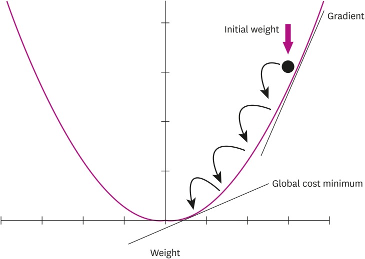
The costs that correspond to given W and b values are shown in the Fig. 1 (obtained from https://rasbt.github.io/mlxtend/user_guide/general_concepts/gradient-optimization/).⁸,⁹,¹⁰ Given the current values of W and b, the gradient is obtained. If the gradient is positive, the values of W and b are decreased. If the gradient is negative, the values of W and b are increased. In other words, the values of W and b determined by the derivative of the cost function.⁸,⁹,¹⁰

Fig. 1. A graph of a cost function (modified from https://rasbt.github.io/mlxtend/user_guide/general_concepts/gradient-optimization/).

ARTIFICIAL NEURAL NETWORK

The basic unit by which the brain works is a neuron. Neurons transmit electrical signals (action potentials) from one end to the other.¹¹ That is, electrical signals are transmitted from the dendrites to the axon terminals through the axon body. In this way, the electrical signals continue to be transmitted across the synapse from one neuron to another. The human brain has approximately 100 billion neurons.¹¹,¹² It is difficult to imitate this level of complexity with existing computers. However, Drosophila have approximately 100,000 neurons, and they are able to find food, avoid danger, survive, and reproduce.¹³ Nematodes have 302 neurons and they survive well.¹⁴ This is a level of complexity that can be replicated well even with today's computers. However, nematodes can perform much better than our computers.

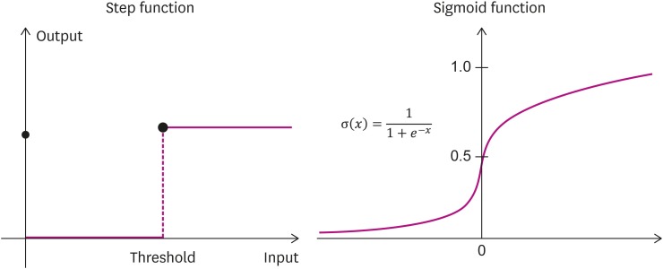
Let's think of the operative principles of neurons. Neurons receive signals and generate other signals. That is, they receive input data, perform some processing, and give an output.¹¹,¹² However, the output is not given at a constant rate; the output is generated when the input exceeds a certain threshold.¹⁵ The function that receives an input signal and produces an output signal after a certain threshold value is called an activation function.¹¹,¹⁵ As shown in Fig. 2, when the input value is small, the output value is 0, and once the input value rises above the threshold value, a non-zero output value suddenly appears. Thus, the responses of biological neurons and artificial neurons (nodes) are similar. However, in reality, artificial neural networks use various functions other than activation functions, and most of them use sigmoid functions.⁴,⁶ which are also called logistic functions. The sigmoid function has the advantage that it is very simple to calculate compared to other functions. Currently, artificial neural networks predominantly use a weight modification method in the learning process.⁴,⁵,⁷ In the course of modifying the weights, the entire layer requires an activation function that can be differentiated. This is because the step function cannot be used as it is. The sigmoid function is expressed as the following equation.⁶,¹⁶

Fig. 2. A step function and a sigmoid function.

$$\mathrm{\sigma }\left(x\right)=\frac{1}{1+e^{-x}}$$

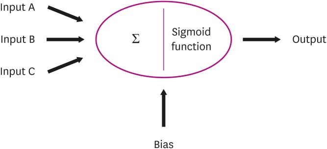
Biological neurons receive multiple inputs from pre-synaptic neurons.¹¹ Neurons in artificial neural networks (nodes) also receive multiple inputs, then they add them and process the sum with a sigmoid function.⁵,⁷ The value processed by the sigmoid function then becomes the output value. As shown in Fig. 3, if the sum of inputs A, B, and C exceeds the threshold and the sigmoid function works, this neuron generates an output value.⁴

Fig. 3. Input and output of information from neurons.

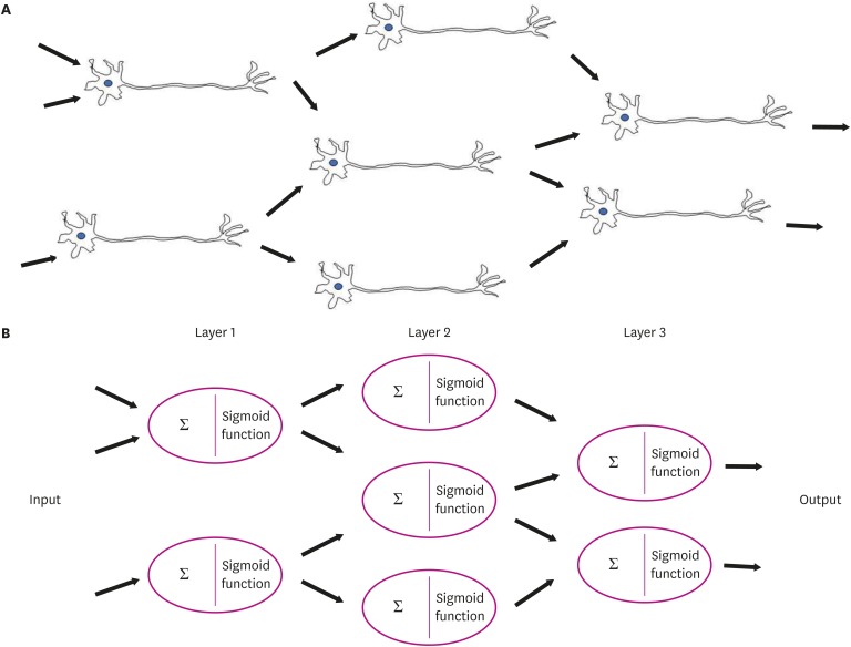
A neuron receives input from multiple neurons and transmits signals to multiple neurons.⁴,⁵ The models of biological neurons and an artificial neural network are shown in Fig. 4. Neurons are located over several layers, and one neuron is considered to be connected to multiple neurons. In an artificial neural network, the first layer (input layer) has input neurons that transfer data via synapses to the second layer (hidden layer), and similarly, the hidden layer transfers this data to the third layer (output layer) via more synapses.⁴,⁵,⁷ The hidden layer (node) is called the “black box” because we are unable to interpret how an artificial neural network derived a particular result.⁴,⁵,⁶

Fig. 4. (A) Biological neural network and (B) multi-layer perception in an artificial neural network.

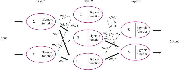
So, how does a neural network learn in this structure? There are some variables that must be updated in order to increase the accuracy of the output values during the learning process.⁴,⁵,⁷ At this time, there could be a method of adjusting the sum of the input values or modifying the sigmoid function, but it is a rather practical method to adjust the connection strength between the neurons (nodes).⁴,⁵,⁷ Fig. 5 is a reformulation of Fig. 4 with the weight to be applied to the connection strength. Low weights weaken the signal, and high weights enhance the signal.¹⁷ The learning part is the process by which the network adjusts the weights to improve the output.⁴,⁵,⁷ The weights W1,2, W1,3, W2,3, W2,2, and W3,2 are emphasized by strengthening the signal due to the high weight. If the weight W is 0, the signal is not transmitted, and the network cannot be influenced.

Fig. 5. The connections and weights between neurons of each layer in an artificial neural network.

Multiple nodes and connections could affect predicted values and their errors. In this case, how do we update the weights to get the correct output, and how does learning work?

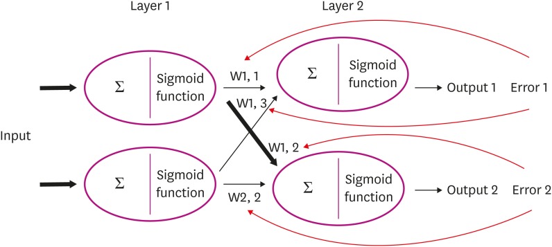
The updating of the weights is determined by the error between the predicted output and the correct output.⁴,⁵,⁷ The error is divided by the ratio of the weights on the links, and the divided errors are back propagated and reassembled (Fig. 6). However, in a hierarchical structure, it is extremely difficult to calculate all the weights mathematically. As an alternative, we can use the gradient descent method⁸,⁹,¹⁰ to reach the correct answer — even if we do not know the complex mathematical calculations (Fig. 1). The gradient descent method is a technique to find the lowest point at which the cost is minimized in a cost function (the difference between the predicted value and the answer obtained by the arbitrarily start weight W). Again, the machine can start with any W value and alter it gradually (so that it goes down the graph) so that the cost is reduced and finally reaches a minimum. Without complicated mathematical calculations, this minimizes the error between the predicted value and the answer (or it shows that the arbitrary start weight is correct). This is the learning process of artificial neural networks.

Fig. 6. Back propagation of error for updating the weights.

CONCLUSIONS

In conclusion, the learning process of an artificial neural network involves updating the connection strength (weight) of a node (neuron). By using the error between the predicted value and the correct, the weight in the network is adjusted so that the error is minimized and an output close to the truth is obtained.

References

- 1.Samuel AL. Some studies in machine learning using the game of checkers. IBM J Res Develop. 1959;3:210–229. [Google Scholar]
- 2.Koza JR, Bennett FH, 3rd, Andre D, Keane MA. Automated design of both the topology and sizing of analog electrical circuits using genetic programming. In: Gero JS, Sudweeks F, editors. Artificial Intelligence in Design. Dordrecht: Kluwer Academic; 1996. pp. 151–170. [Google Scholar]
- 3.Deo RC. Machine learning in medicine. Circulation. 2015;132:1920–1930. doi: 10.1161/CIRCULATIONAHA.115.001593. [DOI] [PMC free article] [PubMed] [Google Scholar]
- 4.Rashid T. Make Your Own Neural Network. 1st ed. North Charleston, SC: CreateSpace Independent Publishing Platform; 2016. [Google Scholar]
- 5.Haykin S, Haykin SS. Neural Networks and Learning Machines. 3rd ed. Upper Saddle River, NJ: Prentice Hall; 2009. [Google Scholar]
- 6.Rashid T, Huang BQ, Kechadi MT. A new simple recurrent network with real-time recurrent learning process; Proceedings of the 14th Irish Conference on Artificial Intelligence & Cognitive Science, AICS 2003; 2003 September 17–19; Dublin, Ireland. place unknown: Artificial Intelligence and Cognitive Science; 2003. pp. 169–174. [Google Scholar]
- 7.Zakaria M, AL-Shebany M, Sarhan S. Artificial neural network: a brief overview. Int J Eng Res Appl. 2014;4:7–12. [Google Scholar]
- 8.Bottou L. Chapter 2. On-line learning and stochastic approximations. In: Saad D, editor. On-Line Learning in Neural Networks. Cambridge: Cambridge University Press; 1999. pp. 9–42. [DOI] [Google Scholar]
- 9.Bottou L. In: Lechevallier Y, Saporta G, editors. Large-scale machine learning with stochastic gradient descent; Proceedings of COMPSTAT'2010: 19th International Conference on Computational Statistics; 2010 August 22–27; Paris, France. Heidelberg: Physica-Verlag HD; 2010. pp. 177–186. [Google Scholar]
- 10.Bottou L. Stochastic gradient descent tricks. In: Montavon G, Orr GB, Müller KR, editors. Neural Networks: Tricks of the Trade. 2nd ed. Heidelberg: Springer-Verlag Berlin Heidelberg; 2012. pp. 421–436. [DOI] [Google Scholar]
- 11.Ebersole JS, Husain AM, Nordli DR. Current Practice of Clinical Electroencephalography. 4th ed. Philadelphia, PA: Wolters Kluwer; 2014. [Google Scholar]
- 12.Shepherd GM, Koch C. Introduction to synaptic circuits. In: Shepherd GM, editor. The Synaptic Organization of the Brain. 3rd ed. New York, NY: Oxford University Press; 1990. pp. 3–31. [Google Scholar]
- 13.Alivisatos AP, Chun M, Church GM, Greenspan RJ, Roukes ML, Yuste R. The brain activity map project and the challenge of functional connectomics. Neuron. 2012;74:970–974. doi: 10.1016/j.neuron.2012.06.006. [DOI] [PMC free article] [PubMed] [Google Scholar]
- 14.Hobert O. Neurogenesis in the nematode Caenorhabditis elegans. WormBook. 2010:1–24. doi: 10.1895/wormbook.1.12.2. [DOI] [PMC free article] [PubMed] [Google Scholar]
- 15.McCulloch WS, Pitts W. A logical calculus of the ideas immanent in nervous activity. 1943. Bull Math Biol. 1990;52:99–115. [PubMed] [Google Scholar]
- 16.Ranka S, Mohan CK, Mehrotra K, Menon A. Characterization of a class of sigmoid functions with applications to neural networks. Neural Netw. 1996;9:819–835. doi: 10.1016/0893-6080(95)00107-7. [DOI] [PubMed] [Google Scholar]
- 17.Kozyrev SV. Classification by ensembles of neural networks. p-Adic Numbers Ultrametric Anal Appl. 2012;4:27–33. [Google Scholar]