Mating system change reduces the strength of sexual selection in an American frontier population of the 19th century

Abstract

Sexual selection, or competition among members of one sex for reproductive access to the other, is one of the strongest and fastest evolutionary processes. Comparative studies support the prediction that sexual selection is stronger in polygamous than in monogamous species. We report the first study of the effect on sexual selection of a change in mating system, from polygyny to monogamy, within a historical human population. Here we show that over the reproductive lifetimes of Utahns born between 1830 and 1894, socially induced reductions in the rate and degree of polygamy correspond to a 58% reduction in the strength of sexual selection. Polygyny conferred a strong advantage to male fitness as well as a weak disadvantage to female fitness. In contrast, mating with multiple males provided little benefit to females in this population. Polygamy benefitted males by increasing reproductive rates and by lengthening reproductive tenure. Each advantage contributed to roughly half of the increased total lifetime reproductive success. This study illustrates both the potency of sexual selection in polygynous human populations and the dramatic influence that short-term societal changes can have on evolutionary processes.

1. Introduction

Sexual selection is the process identified by Darwin (1859) where the members of one sex, generally males, compete with one another for reproductive access to members of the other sex. Theory predicts that sexual selection should be a much stronger evolutionary force in polygamous than in monogamous mating systems (Shuster & Wade, 2003; Wade, 1979; Wade & Shuster, 2004b). Support derives primarily from extensive comparisons across taxa with different mating systems (Andersson, 1994; Bateman, 1948; Jones & Avise, 2001; Lofredo & Borgia, 1986; Shuster & Wade, 2003). We report the first study of the effects on sexual selection of a change in mating system, from polygyny to monogamy, within a population of a single species, Homo sapiens.

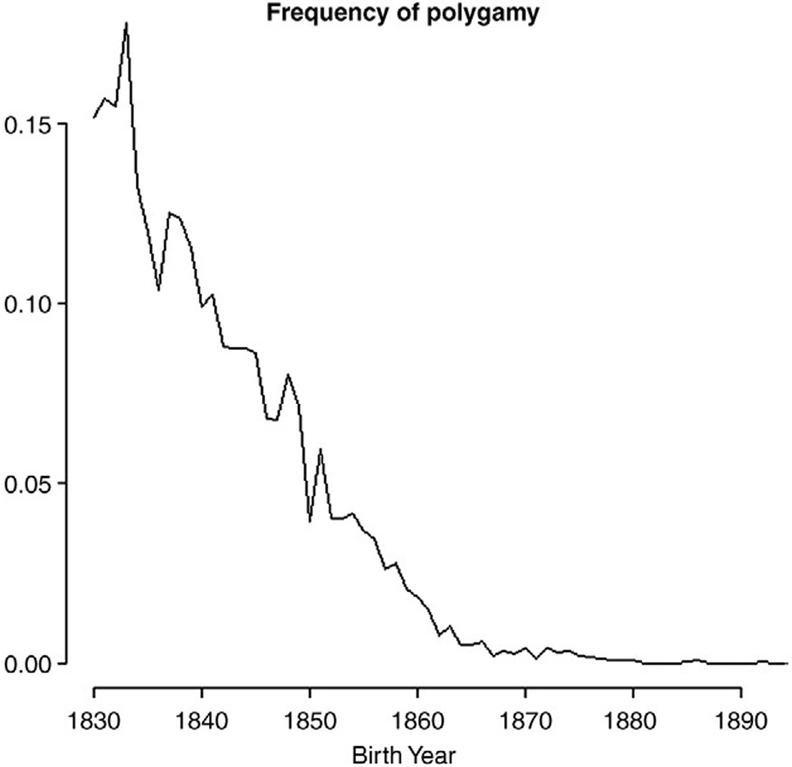
Polygynous marriage, where a man would simultaneously take on multiple wives, was a practice throughout much of the 19th century for some members of the Church of Jesus Christ of Latter-day Saints (LDS or Mormons). In the Utah Territory in the early part of the century, our estimates from the Utah Population Database indicate that the frequency of polygamous men as a fraction of all married men reached a maximum of 17.8% among men born in 1833 (Fig. 1), a figure consistent with previous estimates (Smith & Kunz, 1976). Subsequently, changes in social pressures over the next few decades reduced the frequency of such marriages to less than 1%. New strictures on the practice of polygyny began with the Morrill Anti-Bigamy Act of 1862 outlawing plural marriage throughout the US territories. The US Supreme Court upheld the ban in the face of a freedom of religion challenge in 1878 and, in 1890, the Mormon Church issued the Woodruff Manifesto which officially banned polygyny.

Fig. 1.

Polygamous men in the UPDB as a frequency of all married men by birth year.

Data from this population afford a unique test of the role of polygyny in sexual selection in four ways. First, until now, the primary source of empirical support for sexual selection theory has been comparative studies across taxa with different mating systems (Andersson, 1994; Bateman, 1948; Jones & Avise, 2001; Lofredo & Borgia, 1986; Shuster & Wade, 2003). Second, previous human studies have compared relationships between social mating customs and sexual selection across geographically and culturally distinct populations (Brown, Laland & Mulder, 2009), whereas this study uses temporally defined cohorts that differ in mating system within the same population. Third, our sample size (180,082 parents) is 18 times larger than that in all other human studies of sexual selection combined (Brown et al., 2009), giving unprecedented power to describe sexual selection in a human population. Finally, these data span an important part of the demographic transition (Borgerhoff-Mulder, 1998) where natural fertility conditions prevailed early but reproductive rates rapidly fell over a few generations.

To determine the strength of sexual selection that acts on a population and to best understand how it is influenced by mating system, we need to quantify the associations (e.g., the variances and covariances) between mating success and reproductive success in both males and females. In populations with an equal sex ratio of females to males, the rates of polygyny are necessarily and positively associated with the frequency of males who do not mate (Wade, 1979; Wade & Shuster, 2004b). As a result, polygyny increases the variation among males in mate number (mating success or MS). Using results from fruit fly experiments, Bateman (1948) was the first to argue that variation among males in mate numbers was the most important cause of a sex difference in the variance in reproductive success (RS). Wade (1995) derived the general relationship between the variance in male and female RS, showing that the sex difference in ${\sigma }_{RS}^2$ was a function of male MS. Shuster and Wade (2003) reviewed and extended this theory and applied it to several different taxa (Andersson, 1994; Bjorklund, 1991; Lofredo & Borgia, 1986; Shuster & Wade, 2003), including sex-reversed species with polyandry among territory-holding females (Jones & Avise, 2001), to show how mating system affected the strength of sexual selection. A recent comparative study using 18 geographically diverse human populations, a collection that included both monogamous and polygamous societies (Brown et al., 2009), showed that ${\sigma }_{RS}^2$ and ${\sigma }_{MS}^2$ tended to be higher in males than in females. Following the methods described in the Methods section, we examine these relationships within a single population during a period of change in the practice of plural marriage that affected mating success.

2. Methods

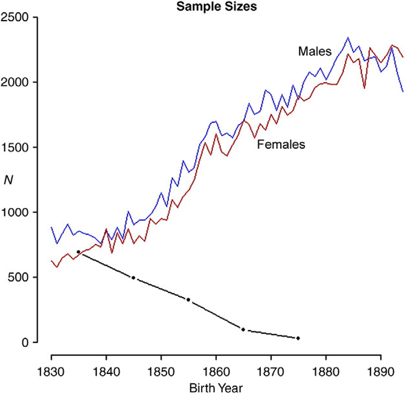
Our extract of the Utah Population Database (UPDB) included birth and death years of the 89,034 fathers and 96,407 mothers recorded in the UPDB born before 1900 (the majority of the UPDB reflecting Utah parents born after 1900 was not available to us). Note that the Utah population was not a strict closed society since potential wives could be recruited via religious conversion and migration into Utah (Daynes, 2001). We used only those individuals with known death year. There were very few individuals born before 1830 and these were excluded from our analysis. Fathers born after 1894 had missing data on their wives who were often born after the cutoff year of 1900. These exclusion criteria meant we had a sample of 72,812 fathers and 75,366 mothers born between 1830 and 1894. Our extract also included the 322,551 sons and 307,754 daughters who were born to parents represented in the UPDB extract. These parents were divided into 65 single birth-year cohorts from 1830 to 1894. Because the UPDB is derived from descendent genealogies, we could not expect it to include reliable counts of nulliparous individuals. We used US census data and a few reasonable assumptions (see Section 2.1 below) to estimate the size of this class of individuals for each sex and birth years. The sample sizes that reflect the total number of parents plus the projected number of nulliparous individuals are illustrated in Fig. A1 in Appendix A.

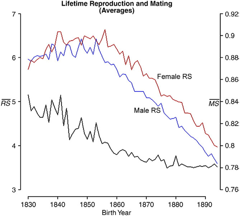
We determined the total number of offspring (reproductive success, ‘RS’) for each individual, the number of his or her reproductive partners (mating success, ‘MS’) and the number of years over which he or she reproduced (reproductive tenure, ‘RT’). The birth year-specific means of mating and reproductive success are shown in Fig. A2 in Appendix A. In addition, each reproductive female was also assigned another value equal to the mating success of the partner that she most often reproduced with. In the cases where females mated with more than one male, the mating success of these females’ first and last mates was also noted. The choice of partner had no noticeable effect on the outcome of our analyses.

2.1. Estimating the number of nulliparous individuals

We need to know the frequency distributions of reproductive success to estimate the strength of sexual selection. This includes those individuals that do not reproduce at all. When information comes from descendent genealogies, such as with the UPDB, these individuals can be undercounted and omitting the zero values diminishes the variance in reproductive success and the strength of selection (Shuster & Wade, 2003). This section explains how we corrected for this bias and estimated the size of the nulliparous populations of males and females.

Our approach was to complement data on survival and reproduction from the UPDB, which we expect to be biased in terms of the relative frequency of reproductive men and women, with information from US census data (Sixteenth Census of the United States, 1943). These data include fertility and marital information about women living in Utah and reported in 1910 and 1940. Parity counts of women relevant to our study period are reproduced in Table 1. These include the age-specific counts of total number of women ever married (W), ever-married women who reported having no children (W₀), ever-married women who did not report number of children (W_U) and single women (S). Women were grouped into age categories of 5-year intervals (e.g., 40 to 44 years of age) until 50 years of age, at which point a 25-year age window was considered. We assumed that marriage and reproductive history did not influence reporting and, in this way, we adjusted for the under-reporting of nulliparous wives by estimating the true counts for nonreproductive women of age interval x and birth-year interval y as ${W^{\prime }}_{xy\left(0\right)}=\frac{W_{xy\left(0\right)}}{1-W_{xy\left(U\right)}/W_{xy}}+S_{xy}$. The adjusted numbers of mothers were ${W^{\prime }}_{xy\left(m>0\right)}=\frac{W_{xy}-W_{xy\left(0\right)}}{1-W_{xy\left(U\right)}/W_{xy}}$, where m>0 indicates fertility.

Table 1.

Fertility and marriage history of Utah women from US Census data

Age class	Birth years	Census year	Women ever married			Single women, S
			Total reporting, W	Zero children, W0	Not reporting, WU
45–49	1891–1895	1940	12,480	1100	1320	520
35–39	1871–1875	1910	8336	627	446	563
40–44	1866–1870	1910	7204	371	372	405
45–49	1861–1865	1910	6244	282	380	240

Always-single women (S) were assumed not to have had children prior to the census year. However, women who were single or married and nulliparous may have had first children after the census. This would cause us to overestimate rates of nulliparity. For this reason, we considered only those women who were 35 years or older at the time of the census. Using reproductive records from the UPDB and pooled overall birth year cohorts of interest (1830–1894), we estimated that the probability that a mother had her first child after 35 was δ₃₅=0.0188. The average taken over the age interval x=35 to 39 (and weighted by age-cohort size at 1910) was δ¯_(35–39), _{(1871–1875)}=0.0119. The corresponding probability for the next youngest age-cohort was δ¯_(30–34), _{(1876–1880)}=0.0406; the chance that missing these mothers may cause problems with our estimates seemed too high to risk using these age cohorts. Women above 49 years of age were not considered owing to the exceedingly large age window (25 years). Although the frequency of missed categorized nulliparous women was gauged to be quite low for the cohorts of interest (between 0.0002 and 0.0119), we made the following adjustments to best account for this bias: $W\text{'}{\text{'}}_{xy\left(0\right)}=W{\text{'}}_{xy\left(0\right)}\left(1-{\overline{\delta }}_{xy}\right)$ and $W\text{'}{\text{'}}_{xy\left(m>0\right)}=W{\text{'}}_{xy\left(m>0\right)}+{\overline{\delta }}_{xy}W{\text{'}}_{xy\left(0\right)}$.

Finally, we accounted for the probability that a women did not survive from birth to the time that the census was taken. Using UPDB data, we estimated the probability L_xy(m>0) that a mother born at time y lived to age x. Using the set of individuals with no reproductive records, we estimated L_xy(0), which better reflected the cumulative survival fraction of the nulliparous females. We reasoned that if the census figures accounted for all females who had died prior to the census and also correctly forecasted the frequency of future first-time mothers, then the total number of mothers and non-reproductive females would be $\frac{{W^{″}}_{xy\left(m>0\right)}}{L_{xy\left(m>0\right)}}$ and $\frac{{W^{″}}_{xy\left(0\right)}}{L_{xy\left(0\right)}}$ respectively, where x was at the age at census and y was the the birth year. The relative frequencies of projected always-nulliparous females born in birth year interval y, P_y(F), as well as all parameter estimates from the UPDB that were used in the necessary adjustments described above, are shown in Table 2.

Table 2.

Cohort-specific factors estimated from the UPDB used to estimate the size of the nulliparous fraction of females

Age class	Birth years	Census	${\overline{\delta }}_X$	${\overline{L}}_{XY\left(m=0\right)}$	${\overline{L}}_{XY\left(m>0\right)}$	PY(F)
45–49	1891–1895	1940	2.1510E–04	0.5259	0.8954	0.1897
35–39	1871–1875	1910	1.1860E–02	0.4683	0.9326	0.2281
40–44	1866–1870	1910	2.3040E–03	0.4322	0.9054	0.1876
45–49	1861–1865	1910	2.8220E–04	0.3771	0.8679	0.1637

US Census data and UPDB data were binned into 5-year and 1-year windows, respectively. To account for this, single-year values of δ_x, L_xy(m=0) and L_xy(m>0) were averaged over 5 years (and weighted by cohort size) to arrive at the values above.

We regressed P_y(F) onto the midpoint of the 5-year birth intervals in order to project nulliparous fractions on specific birth years, including those not included in the census study. After weighting by the size of the informative census sample (W_xy+S_xy), we estimated the least squares best linear fit to be P_y(F)=−.207+2.1370E−04×y, which predicted a very gradual increase in the relative size of the ever-nulliparous population from 0.184 in 1830 to 0.198 in 1894. We applied these estimates to our counts of mothers from the UPDB to estimate the true size of the female nulliparous population in the Utah population.

As no such census information was available for Utah males, we had to infer the frequency of nulliparity from the female results. We assumed that mean MS, adjusted for unequal sex ratios at birth, was the same for both sexes born at the same time. This need not be absolutely true if some sex and birth year cohorts are simply more successful than others, but because each new individual must have one father and one mother, we expect that this is a fair assumption over the long-term. Following this argument, the nulliparous fraction of males born at Y is

$$P_Y\left(M\right)=1-\frac{\overline{{\text{MS}}_Y}\left(\text{females}\right)}{R\times \overline{{\text{MS}}_Y}\left(\text{fathers}\right)},$$ (1)

where R is the sex ratio at birth, which we estimate to be 1.048 based on the UPDB records.

3. Results

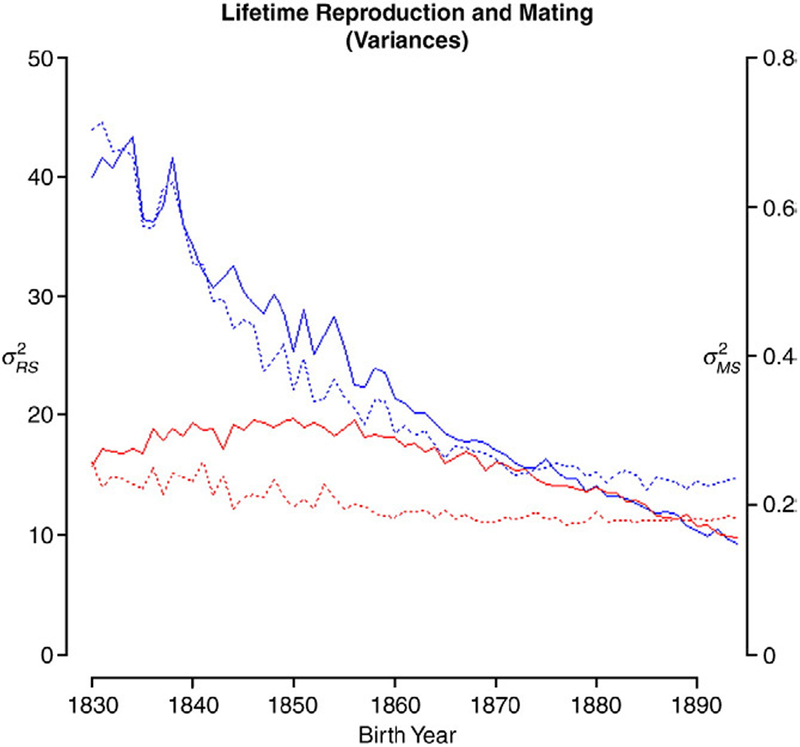
We observe pronounced sex differences in the variation in RS among those born in the early 1830s (years indicate time of birth unless otherwise indicated) (Fig. 2). The average variance taken over the first 5 years (1830–1834) is nearly 2.5 times higher in males than in females [${\sigma }_{RS}^2$ (♂)=41.6, ${\sigma }_{RS}^2$ (♀)=16.8]. There is an overall decline in female variation with increasing birth year [${\sigma }_{RS}^2$(♀)=10.6 in the early 1890s, a decline of 37%]. Over this same 65-year period, male ${\sigma }_{RS}^2$ declined by 75.6% (to 10.2), roughly converging with that of females. Most of the decline occurred prior to 1860, in the period leading up to and coincident with the birth of males that reached reproductive maturity after the 1862 ban on polygyny.

Fig. 2.

Variation in lifetime reproductive success (solid line and left axis) and mating success (dotted line and right axis) for males (black [blue]) and females (grey [red]) by birth year.

The variation in mating success, or number of mates, mirrors the pattern for RS (Fig. 2), although female variation appears not to change much over the study period. Male ${\sigma }_{MS}^2$ (0.687) was nearly three times higher than that of females (0.237) in the early 1830s but only 25.9% higher in the early 1890s (0.227 vs. 0.181). Male ${\sigma }_{MS}^2$ dropped 66.9% from the first to last 5 years of the study, while female ${\sigma }_{MS}^2$ lost 23.5% over this time, although this latter figure represents a very small absolute change in the variance. As with reproductive success, the male decline in the variance of mating success was most rapid leading up to the early 1860s.

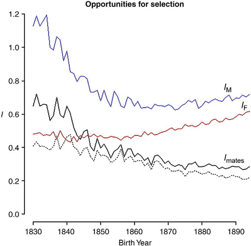
Declines in the sex-related differences in ${\sigma }_{RS}^2$ co-occur with change in the frequency of polygamy. Direct causality cannot be ensured, however, because mean reproduction declines over the study period. Crow’s index for the opportunity for selection $I={\sigma }_{RS}^2/{\overline{\text{RS}}}^2$ measures variance in relative fitness and sets an upper limit on the rate of evolutionary change (Crow, 1958; Wade, 1979; Wade & Shuster, 2004a). Based upon Fisher’s (1930) Fundamental Theorem of Natural Selection, Crow’s index arises from the earliest formulations of evolutionary genetics. Because it is standardized by mean reproduction, this comparative measure is more appropriate for identifying secular changes over segments of the demographic transition, or times where mean reproduction changes rapidly, because changes in mean fitness cannot, by themselves, change I. The variance in mate number among males weighted by the ratio of squared sex-specific mean RS, $I_{mates}={\left(\frac{\overline{\text{RS}}\left(\text{females}\right)}{\overline{\text{RS}}\left(\text{males}\right)}\right)}^2{\sigma }_{\text{MS}}^2$ is a useful comparative metric often called the opportunity for sexual selection (Shuster & Wade, 2003; Wade, 1995). The strength of selection on males I_M (which includes I_mates) was 1.160 in the early 1830s but fell rapidly to 0.699 in the early 1850s and then increased slightly to 0.706 over the next three decades. The strength of selection on females (I_F), which does not include sexual selection, was less than half that of I_M in the early 1830s (0.482, or 41.5% of I_M), remained fairly constant into the late 1860s and then increased slightly to 0.601 over the next three decades. As a result of these secular changes, the opportunity for sexual selection I_mates was greatest in the early 1830s (0.667), dropped by 42.4% in the ensuing two decades (0.384 in the early 1850s) and converged towards one-quarter at the end of the 19th century (0.279 in the early 1890s). Thus, the opportunity for sexual selection, I_mates, lost 58.2% of its strength coincident with the change in mating system from polygyny to monogamy (Fig. 3).

Fig. 3.

The opportunity for selection for males (I_M, blue) and females (I_F, red) by birth year. The solid black line is the opportunity for sexual selection I_mates, and the black dotted line represents the proportion of all selection explained by sexual selection. The strength of sexual selection decreases markedly over time, both in absolute terms and as a proportion of all selection.

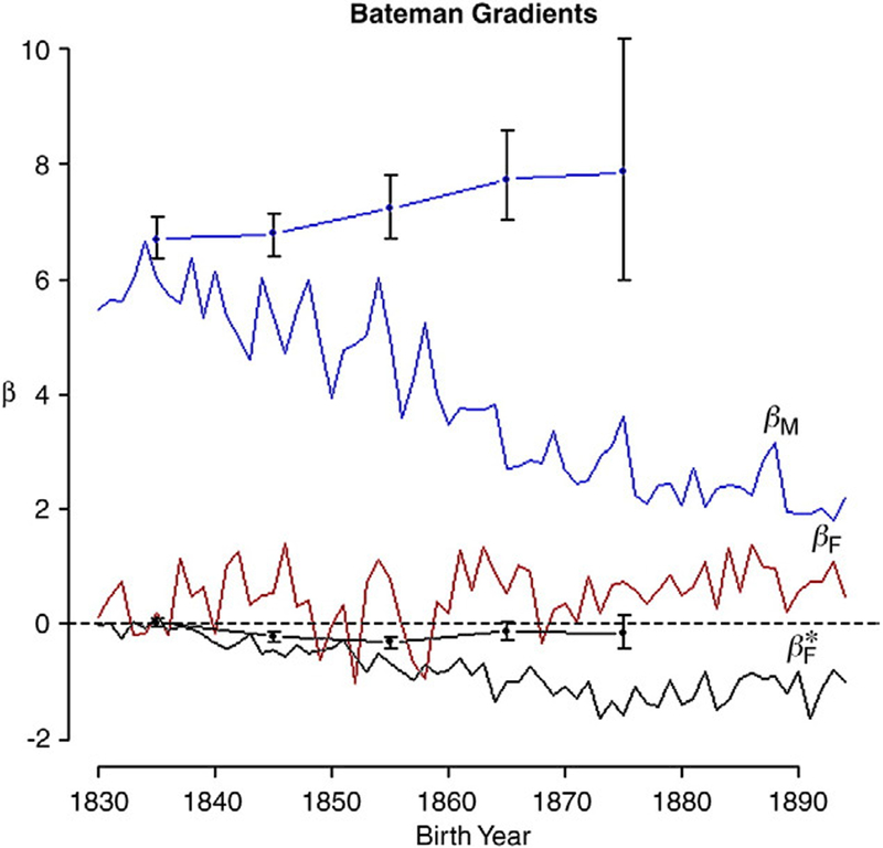
We can estimate the reproductive costs and benefits of polygyny, for both males and females, by studying their Bateman gradients. These are the marginal effects of mating system on reproductive success for each sex, estimated from the year-specific slope of the linear regression of RS on MS ($\beta ={\sigma }_{MS,RS}/{\sigma }_{RS}^2$ , conditioned on MS≥1). Differently put, these are the sensitivities of parents’ reproductive success to changes in mating success. Until now there was insufficient evidence to characterize the associations between reproductive and mating success within both sexes (Brown et al., 2009). The UPDB now gives us unprecedented power to describe these relationships in a human population. In our analysis, we find that the Bateman gradients change with birth year (Fig. 4). Male gradients (β_M) are highest in the 1830s, averaging 5.87 in the first 5 years (i.e., by taking on one additional reproductive mate, the average father would have increased his reproductive success by nearly six offspring). However, β_M diminishes linearly with birth year to 1.92 by the early 1890s.

Fig. 4.

Bateman gradients by birth year (β_M is blue, β_F is red and β_F* is black). Dotted lines and error bars correspond to estimated gradients when serial monogamists are excluded from the analysis. These are grouped by decade of birth. Of these, the upper (blue) line corresponds to β_M and the lower black line to β_F* Error bars represent the 95% confidence intervals estimated by bootstrapping over parents (using the adjusted bootstrap percentile method in R version 2.10.1 ‘boot’ package; Canty & Ripley, 2009; Davison & Hinkley, 1997; R Development Core Team, 2009) . In terms of fitness, polygyny strongly benefits males but weakly harms females.

We can also describe the analogous relationship between RS and MS for females (β_F). It is weakly positive and increases slightly over the 65 birth-year cohorts (from 5-year means of 0.195 to 0.671; Fig. 4), indicating that increasing the number of males with whom a female mates had a small, but real, benefit on female reproductive fitness. This benefit increased slightly over the study period. Multiple mating in these females did not follow from polyandry; it is likely a result of widowed or divorced mothers who remarried before having more children.

In his classic 1969 article on the origin of polygyny, Orians (1969) suggested that polygynous females face the cost of having to share limiting resources with other females mated to the same male. They do so to their advantage, however, if the benefits (for example, mating with a male that is of higher than average quality) outweigh that cost. To assess the effects of polygyny on females, we calculated a third Bateman gradient, β*_F, which describes the effect of male mating success on the reproductive success of his mates. A positive β*_F means that females benefit from sharing the same mate with other females. A negative value means that the relationships among females who share mates are antagonistic or competitive with respect to reproductive success (Wade, 1979). Between 1830 and 1834, there was a small negative β*_F (the 5-year average was −0.06). Over the next four decades, it became progressively more negative, reaching a low of −1.36 in the late 1870s and then rising to −1.11 in the early 1890s (Fig. 4). That is, for the average mated women born in the late 19th century, sharing a mate with an additional female would have reduced her number of offspring by slightly more than one.

Male mating success is not a perfect indicator of polygamy in any species, including humans. Widowers with two non-overlapping reproductive wives in sequence would have higher than average MS without being polygamists, for example. Nevertheless, these individuals and polyga-mists contribute to the Bateman gradients. The clear trend showing that increased MS benefits men less with increased birth year may not necessarily indicate a secular reduction in the benefits of polygamy to males. Instead, changes in β_M may reflect a change in the relationship between mating system and mating success. While the frequency of polygamy declined over time in this population, monogamist males would still have remarried to replace deceased or divorced reproductive partners. Over time, these serial monogamists (men who married more than once but never had more than one wife at a time) comprised an ever-growing proportion of all males with MS>1. Compared to males born early in the 19th century, MS in later-born males increased largely by mate replacement (rather than mate accumulation), meaning that it was the older [and presumably less fertile — see Ford et al. (2000)] men from these age cohorts who gained high mating success. Similar alternative explanations may account for the decline in β*_F with time. Women in multi-wife households who were born in the late 19th century may have suffered increased reproductive constraints compared to their earlier counterparts. However, it is also possible that later birth years brought a larger proportion of women whose early deaths elevated their mate’s MS by precipitating their remarriage. Alternatively, they may have themselves married widowers who are older on average and may have reduced fertility.

To address these issues, we recalculated β_M and β*_F using only those fathers (and their mates) who either (1) reproduced with only one woman (MS=1) or (2) were identified in the UPDB as being polygamists. This effectively removed from the analysis those monogamist fathers with MS>1. Polygamists with multiple reproductive partners became extremely rare towards the end of the 19th century (Fig. 1). For this reason, we grouped parents into cohorts based upon the decade of birth instead of single years of birth (sample sizes are shown in Appendix A Fig. A1), ending with birth years 1870–1879. Otherwise, we re-analyzed Bateman gradients as before.

One might expect social pressures late in the 19th century to impose some additional cost to polygamist males that would cause β_M to decrease with time. In fact, we see no secular changes in β_M, suggesting that the relative benefit to males of polygamy remained high over the time spanning this study. One likely explanation for this is that, after polygamy was outlawed in the Utah Territory, some individuals who opposed the ban continued to engage in polygamy in Utah while others immigrated to other locations including Mexico and Canada where marriage practices were less likely to be regulated. This subset of parents in the UPDB had an outsized contribution to β_M in the latter part of the 19th century as they were likely the major source of polygamists. Subject to reproductive constraints more closely resembling polygamists born in the early part of the 19th century instead of their Utah-dwelling contemporaries, they married and reproduced accordingly (Fig. 4).

As with the male Bateman gradient, the gradient that measures the association between female RS and her mate’s MS, β*_F, changed little when monogamist males with multiple mates were excluded from the analysis. Polygamy conferred a slight, but insignificant, cost to female reproduction in the first decade of births (the 1830s). These costs increased and became significant in the ensuing two decades. In the birth decades of the 1860s and 1870s, β*_F remained negative but the 95% confidence intervals associated with estimates were too wide to show significance. Loss of significantly negative β*_F values may have followed from the dramatic reduction in the sample size of polygamists in these later cohorts rather than a real change in the cost of polygamy to females.

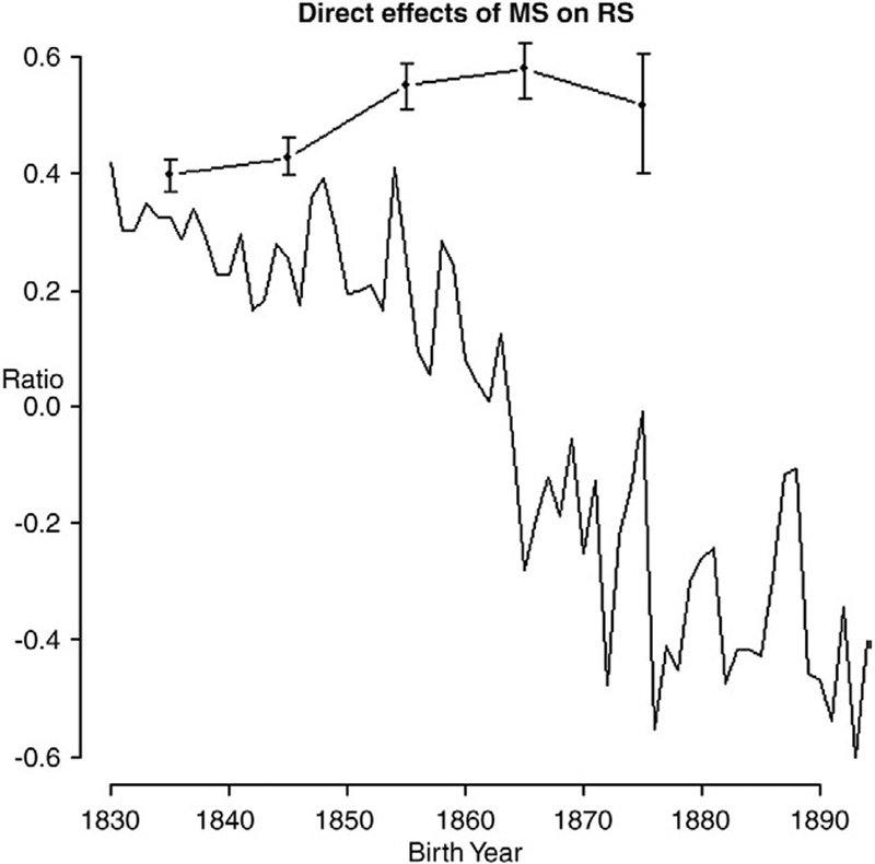
Mating success and polygamy improve men’s fitness. Multiple wives can either (1) enhance male reproductive rates, increasing the fertilization opportunities at any one time, or (2) lengthen the reproductive tenure (RT) of the husband by offering him reproductive opportunities over a greater span of time. To determine the relative importance of each, we calculated the partial covariance between male MS and RS, holding RT constant. The ratio of the partial covariance to the total covariance is the fraction of the association between male MS and RS that is explained by changes in reproductive rates. We find that the ratio was initially positive (0.340 in the early 1830s), decreased until it became negative in the late 1860s (−0.167) and finally reached a low of −0.481 in the early 1890s (Fig. 5). This suggests that high male MS increased both the reproductive rates and reproductive tenures (RT) of males born early in the 19th century. The effects become antagonistic in males born later; increased MS decreased the per-year contributions to RS but increased a male’s RT.

Fig. 5.

Relative effect of MS on RS that is caused by increasing the reproductive rate of males. The lower black line uses all data grouped into birth-year cohorts. The upper black line with dots and error bars (95% confidence intervals — see Fig. 4 legend) excludes monogamous men with MS>1. These are grouped into birth decades. Roughly half of the male benefit of polygyny derives from increased male reproductive rates; the remainder of the fitness advantage follows from the increased time over which children are fathered.

As we observed with the Bateman gradients, changes in the relative contribution of reproductive rate vs. reproductive tenure could be due to secular changes in the relationship between mating system and mating success. As before, we investigated this possibility by repeating the analysis after eliminating monogamist males who reproduced with multiple females. Polygamy increased reproductive success by lengthening reproductive tenure and increasing per-year reproductive rates by roughly equal degrees. In the first two birth decades (1830s and 1840s), 39.7% and 42.7% of the benefit of MS to RS in males follow directly from increasing reproductive rates. The increase in rate effects on RS increased significantly in the following two birth decades (55.2% and 57.9%). This increase differs markedly from the negative effect observed from the more inclusive analysis that includes serial monogamists.

4. Discussion

Our study confirms the three predictions of sexual selection theory (Bateman, 1948; Shuster & Wade, 2003; Wade, 1979; Wade & Shuster, 2004b) in relation to mating system: (1) male ${\sigma }_{RS}^2$ is greater than female ${\sigma }_{RS}^2$; (2) male ${\sigma }_{MS}^2$ is greater than female ${\sigma }_{MS}^2$; and (3) the association between MS and RS is stronger in males than in females. For males, polygamy increases reproduction by lengthening the span over which they mate and by increasing reproductive rates. Both effects contribute to reproduction in roughly equal measure. For females, the association between female RS and MS (β_F) is weak, especially so early in the 19th century when the population presumably more closely experienced natural fertility conditions. Applied to recent humans at least, results from this population seem to favor early views of female MS that de-emphasize its value to fitness over the more recent perspectives that stress its adaptive value (Hrdy, 1997; Jennions & Petrie, 2000; Wolff & Macdonald, 2004). This interpretation might not be applicable to all human populations as evidence from other human datasets suggests that the direction of the relationship between female MS and RS may be culture specific (Brown et al., 2009). Finally, we observe that, on average, a female’s RS declines as her mate’s MS increases (β*_F<0), suggesting a fitness cost of polygamy to females. This contrasts to consistently high male benefits of polygamy and provides key evidence in support of the polygyny threshold model (Orians, 1969). Earlier work on this historical Utah population has shown a similar pattern of reduced fertility in females involved with plural marriages (Anderton & Emigh, 1989; Bean & Mineau, 1986).

This work bears on the applicability of Alexander’s (1979, 1987) influential ideas on the role of male choice to the evolution of human mating systems. Alexander proposed that cooperation between males is opposed by high male reproductive variance and that this intense conflict suppresses the establishment of effective social functions. Monogamy that is imposed on males by males is viewed as one way by which within-group competition is lessened to the advantage of the competitive value of the population as a whole.

Our findings indicate that the choice to forgo the opportunity to be polygamous can be very expensive in terms of fitness, at least for those males who have the capacity and competitive means to have many females. Because the interests between the most powerful and influential males and the group as a whole are in conflict, the fitness advantages gained by societies by banning the practice may also be large if cooperative restraints on polygamy are to be favored by natural selection. In the case of members of the LDS church in Utah, however, the imposition of monogamy originated outside the group rather than from the social organization of reproductively competing males within the group. Further work should be done to test the feasibility of Alexander’s ideas, especially comparative analyses that describe the relationships between rates and incidence of polygamy and population growth rates across many societies. Explicit multi-level selection models should be developed to better understand what biological and social conditions are necessary to allow the evolution of monogamy by Alexander’s mechanism.

Notably, the sex differences in reproductive and mating success decreased as laws and religious customs changed during the latter half of the 19th century, causing individuals to become less likely to adopt a polygamous lifestyle. One result is that the decrease in male ${\sigma }_{MS}^2$ eliminated over 58% of the opportunity for sexual selection (Fig. 3). Over this time, the proportion of all selection caused by sexual selection,$\frac{p{I}_{mates}}{p{I}_m+\left(1-p\right)I_{\text{F}}}$ [where p=R/(R+1) is the frequency of males born], fella 5-year average of 41.2% (in 1830– 1834) to just 22.1% (1890–1894). Interestingly, the estimate from early in the 19th century is congruent with the estimated range of 28.4% to 77.7% from Y-chromosome and mitochondrial sequence data from other human populations (Wade & Shuster, 2004a).

Appendix A

Fig. A1.

Sample sizes by birth year for males (blue) and females (red), including the projected nulliparous individuals. The black line represents the sample size of polygamous men with MS>1. These are grouped into birth decades.

Fig. A2.

Mean reproductive and mating success. Males and female RS (blue and red, respectively) correspond to the left axis. Mean female mating success corresponds to the right axis. As we explain in the Methods section, we have assumed that mean male mating success is 4.8% higher.

References

- Alexander RD (1979). Darwinism and human affairs. Seattle: University of Washington Press, p. 317. [Google Scholar]
- Alexander RD (1987). The biology of moral systems. Hawthorne, NY: A. de Gruyter, p. 301. [Google Scholar]
- Andersson MB (1994). Sexual selection. Princeton, NJ: Princeton University Press, p. 624. [Google Scholar]
- Anderton DL, & Emigh RJ (1989). Polygynous fertility — sexual competition versus progeny. American Journal of Sociology, 94(4), 832–855. [DOI] [PubMed] [Google Scholar]
- Bateman AJ (1948). Intra-sexual selection in Drosophila. Heredity, 2(3), 349–368. [DOI] [PubMed] [Google Scholar]
- Bean LL, & Mineau GP (1986). The polygyny-fertility hypothesis: A re-evaluation. Population Studies, 40(1), 67–81. [DOI] [PubMed] [Google Scholar]
- Bjorklund M (1991). Evolution, phylogeny, sexual dimorphism and mating system in the Grackles (Quiscalus Spp, Icterinae). Evolution, 45(3), 608–621. [DOI] [PubMed] [Google Scholar]
- Borgerhoff-Mulder M (1998). The demographic transition: Are we any closer to an evolutionary explanation? Trends in Ecology & Evolution, 13(7), 266–270. [DOI] [PubMed] [Google Scholar]
- Brown GR, Laland KN, & Mulder MB (2009). Bateman’s principles and human sex roles. Trends in Ecology & Evolution, 24(6), 297–304. [DOI] [PMC free article] [PubMed] [Google Scholar]
- Canty A, & Ripley B (2009). boot: Bootstrap R (S-Plus) Functions. R package version. Version 1.2–38.
- Crow JF (1958). Some possibilities for measuring selection intensities in man. Human Biology, 30, 1–13. [PubMed] [Google Scholar]
- Darwin C (1859). On the origin of species by means of natural selection.London: John Murray, p. 512. [Google Scholar]
- Davison AC, & Hinkley DV (1997). Bootstrap methods and their applications. Cambridge: Cambridge University Press, p. 582. [Google Scholar]
- Daynes KM (2001). More wives than one: transformation of the Mormon marriage system, 1840–1910. Urbana: University of Illinois Press; x, 305 p. [Google Scholar]
- Fisher RA (1930). The genetical theory of natural selection. Oxford:Clarendon Press. [Google Scholar]
- Ford WCL, North K, Taylor H, Farrow A, Hull MGR, Golding J, et al. (2000). Increasing paternal age is associated with delayed conception in a large population of fertile couples: Evidence for declining fecundity in older men. Human Reproduction, 15(8), 1703–1708. [DOI] [PubMed] [Google Scholar]
- Hrdy SB (1997). Raising Darwin’s consciousness — Female sexuality and the prehominid origins of patriarchy. Human Nature-an Interdisciplinary Biosocial Perspective, 8(1), 1–49. [DOI] [PubMed] [Google Scholar]
- Jennions MD, & Petrie M (2000). Why do females mate multiply? A review of the genetic benefits. Biological Reviews, 75(1), 21–64. [DOI] [PubMed] [Google Scholar]
- Jones AG, & Avise JC (2001). Mating systems and sexual selection in male-pregnant pipefishes and seahorses: Insights from microsatellite-based studies of maternity. Journal of Heredity, 92(2), 150–158. [DOI] [PubMed] [Google Scholar]
- Lofredo CA, & Borgia G (1986). Sexual selection, mating systems, and the evolution of avian acoustical displays. American Naturalist, 128(6), 773–794. [Google Scholar]
- Orians GH (1969). On evolution of mating systems in birds and mammals.American Naturalist, 103(934), 589–603. [Google Scholar]
- R Development Core Team (2009). R: A language and environment for statistical computing. Vienna, Austria: The R Foundation for Statistical Computing. [Google Scholar]
- Shuster SM, & Wade MJ (2003). Mating systems and mating strategies. Princeton, NJ: Princeton University Press, p. 520. [Google Scholar]
- Sixteenth Census of the United States. (1943). Population Differential fertility 1940 and 1910. Washington DC: Government Printing Office. [Google Scholar]
- Smith JE, & Kunz PR (1976). Polygyny and fertility in nineteenth-century America. Population Studies, 30, 465–480. [PubMed] [Google Scholar]
- Wade MJ (1979). Sexual selection and variance in reproductive success.American Naturalist, 114(5), 742–747. [DOI] [PubMed] [Google Scholar]
- Wade MJ (1995). The ecology of sexual selection — mean crowding of females and resource-defense polygyny. Evolutionary Ecology, 9(1), 118–124. [Google Scholar]
- Wade MJ, & Shuster SM (2004a). Estimating the strength of sexual selection from Y-chromosome and mitochondrial DNA diversity. Evolution, 58(7), 1613–1616. [DOI] [PubMed] [Google Scholar]
- Wade MJ, & Shuster SM (2004b). Sexual selection: Harem size and the variance in male reproductive success. American Naturalist, 164(4), E83–E89. [DOI] [PubMed] [Google Scholar]
- Wolff JO, & Macdonald DW (2004). Promiscuous females protect their offspring. Trends in Ecology & Evolution, 19(3), 127–134. [DOI] [PubMed] [Google Scholar]