Advanced approaches for quantitative characterization of thermal transport properties in soft materials using thin, conformable resistive sensors

Abstract

Noninvasive methods for precise characterization of the thermal properties of soft biological tissues such as the skin can yield vital details about physiological health status including at critical intervals during recovery following skin injury. Here, we introduce quantitative measurement and characterization methods that allow rapid, accurate determination of the thermal conductivity of soft materials using thin, skin-like resistive sensor platforms. Systematic evaluations of skin at eight different locations and of six different synthetic skin-mimicking materials across sensor sizes, measurement times, and surface geometries (planar, highly curvilinear) validate simple scaling laws for data interpretation and parameter extraction. As an example of the possibilities, changes in the thermal properties of skin (volar forearm) can be monitored during recovery from exposure to ultraviolet radiation (sunburn) and to stressors associated with localized heating and cooling. More generally, the results described here facilitate rapid, non-invasive thermal measurements on broad classes of biological and non-biological soft materials.

GRAPHICAL ABSTRACT

1. Introduction

1.1.

Skin is a critical, multi-purpose organ within the integumentary system [1]. Accounting for 12–15 percent of the total body weight, the skin serves many purposes such as a: (1) protective barrier against pathogens and microbes, (2) sensory interface to the surrounding environment (i.e. touch, heat, cold, pain), and (3) physiology regulator (hydration, sweat, hair, Vitamin D synthesis, and temperature etc.) [2]. Devices, particularly wearable systems, for measuring the thermal properties of the skin can provide vital information about physiological health status. Designs that (1) minimize the mechanical mismatch at the skin–device interface,(2) maximize conformal contact between skin and device, (3) eliminate any constrains in natural motions of the skin, (4) avoid any thermal load on the skin and (5) operate in a physically imperceptible, non-irritating manner are particularly attractive [3–12]. Recent reports describe approaches to such skin-like, or ‘epidermal’, devices and outline their capabilities for precision, continuous measurements of hydration, cutaneous wound healing, blood flow, temperature, thermal conductivity and thermal diffusivity [13–24].

The following describes the development, validation and application of advanced methods for using such devices in a transient plane source (TPS) mode [25] to yield the thermal conductivity in a computationally efficient, accurate manner that avoids experimental uncertainties associated with previous approaches. An application example focuses on characterization of erythema as a sign of skin injury. Erythema is a physiological phenomenon characterized by a reddening of the skin caused by vasodilation of near-surface capillaries that appears following exposure to heat/cold stresses, pressure, infection, inflammation, allergic reaction, and prolonged exposure to solar radiation (sunburn) [25]. Results show that the near-surface thermal conductivity changes in a manner that can be used for non-invasive monitoring of erythema recovery, of utility for diagnostic and prognostic purposes.

2. Materials and methods

2.1. Fabrication of the sensor and its operating principles

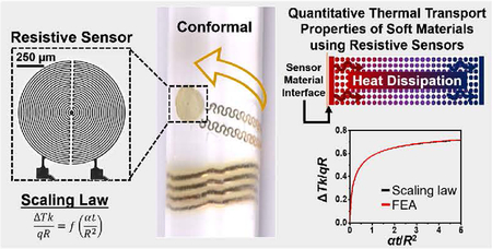
The device architecture consists of a resistive sensor formed with photolithographically defined serpentine metal wires (15–20 μm wide; Cr/Au 8/100 nm thick), as reported previously (see supporting information, SI, for complete fabrication guidelines). An expanded view illustration and a microscope image are in Fig. 1a. The resistive sensors have circular layouts with radii selected between 0.5 and 2.0 mm. The wire connecting the resistive sensor to the power source has a serpentine geometry consistent with design rules in epidermal electronics (100 μm wide; Ti/Cu/Ti/Au 8/550/8/25 nm thick) [3–12]. Encapsulating layers of polyimide (∼4 μm thick; Dow Chemical Co.) above and below place the sensing element in the neutral mechanical plane of the assembly, thereby shielding it from strain-induced resistance changes [3–12]. An ultra-soft (shore-A 00 with ∼60 kPa Young’s modulus), thin film of silicone (50 ± 10 μm thickness; Ecoflex, Smooth-On) chemically adheres to both sides of the device to produce a reusable and mechanically conformal system compatible with deployment on flat or curvilinear surfaces. As a visual example of the high degree of conformality to surfaces, separate digital images display a representative device wrapped around the 4th digit of a left hand, and woven through three parallel, transparent glass rods (rod radii: 1.3 mm) in an over-under-over surface lamination, Fig. 1b–c, respectively.

Fig. 1.

Device components and validation. (a) Schematic illustration of the resistive sensor device layers. (b) Digital image of resistive sensor device laminated on the ring finger of Subject’s left hand. Inset: Optical microscope image of actuator/sensor demonstrating the pattern of the resistive wire (scale bar 250 μm). (c) Optical image of two devices with different actuator/sensor sizes threaded between a series of three transparent glass rods such that the device is draped over the two outermost rods and positioned under the middle most rod.

During operation, the sensor acts as a thermal actuator upon application of direct electrical current (Keithley 6220, A Tektronix Co.). The device connects to the current source by bonding to a conductive ribbon (250 μm spacing, 3M) and small PC board (∼2.5 cm × 5 cm). With thermal actuation, the resistive sensor undergoes self-heating where the resistance of the sensor linearly increases with temperature per the coefficient of resistance of the metal (Au), Figure S3. Direct conversion between resistance and temperature is achieved by device calibration. Each device is calibrated by measuring its resistance at five different temperatures, then plotting temperature vs. resistance to determine the slope. An infrared camera (FLIR One) is used to determine temperature.

2.2. Models for finite element analysis of thermal transport

Finite element analysis (FEA) modeling exploits commercial software ABAQUS [26] to capture the thermal response of the device on flat and curved-cylindrical samples. Inputs for FEA include approximations in conjunction with known and experimentally determined parameters. The known and experimental parameters include: (1) the thickness, and thermal conductivity (k) and diffusivity (α) of the two encapsulation layers, polyimide (4 μm thick, k = 0.52 W/mK, α = 0.32 mm²/s [17,27]) and Ecoflex (50 μm thick, k = 0.21 W/mK, α = 0.11 mm²/s [17]), and (2) the temperature change (ΔT) due to thermal actuation across select time points (i.e. ΔT at 2 s, 20 s, and 40 s etc.). FEA inputs also include: (A1) approximate resistive sensor area, and (A2) room air convection coefficients and (A3) the thermal diffusivity (α) of the sample materials, which are assumed from literature or commercial standards. In the case of A1, the resistive sensor is treated as a circular surface with homogeneous outer contour and power. The FEA with and without the round resistive sensor approximation differs by only 1%, Fig. 2a–b. This approximation is valuable because it reduces the computation time. In the case of A2, a simple bench-experiment involving two different devices aids in the determination of the appropriate convective heat transfer coefficients that correspond to airflow over the device. Briefly, the first device, encapsulated with the normal Ecoflex thickness (50 μm), is laminated directly on a large, thick (10 mm), flat sample of Ecoflex (i.e. sample is considered a semi-infinite plane). Two different airflow environments (controlled and uncontrolled) are used when collecting experimental measurements: (1) controlled(i.e. a glass enclosure is placed over the device, protecting it from the low forced-flow of room air conditioning), and (2) uncontrolled(i.e. the forced convection airflow from standard room air conditioning is allowed to flow over the device). The second device, encapsulated on both the top and bottom sides with excess Ecoflex such that a semi-infinite plane can be considered for both sides of the device, allows for an effective air convection coefficient of 0 W/m² K during heating. All other experimental conditions are the same for both devices. FEA is used to evaluate the point of minimum error (%) for both airflow environments considered with device 1 to determine the appropriate air convection coefficients. Based on minimum error FEA simulation, 6 W/m² K is the thermal coefficient for the “controlled” airflow case (this value is used in all FEA simulations unless otherwise noted) and 15 W/m² K is the thermal coefficient for the “uncontrolled” airflow case, Fig. 2c–d.

Fig. 2.

Determination of the air convection coefficient. (a) Simulated plot of the change in temperature as a function of time (s) showing good agreement between FEA that considers the actual sensor shape (red line) vs. a sensor shape approximated as a circle (black line). (b) A top-view illustration of the actual (left) and approximated (right) sensor shapes, and a side-view illustration of a sensor atop a sample (bottom). (c) Illustrations showing the experimental set-ups for validation of air convection approximations. (d) Plot of simulated error % as a function of air convection (W/m²K) for both ‘covered’ (black line; 6 W/m²/K) and ‘un-covered’ (dotted line; 15 W/m²K) interpreted from experiment data-sets. (For interpretation of the references to color in this figure legend, the reader is referred to the web version of this article.)

The error between FEA and experimental data is minimized with respect to k for a given α. Here the error is defined as

$$Error=\sqrt{\frac{1}{t_{total}}{{\displaystyle {\int }_0^{t_{total}}\left(\frac{\Delta T_{Exp}-\Delta T_{FEA}}{\Delta T_{FEA}}\right)}}^{2}dt,}$$ (1)

where ΔT_Exp and ΔT_FEA are temperature increases in the experiment and FEA, respectively, and t_total is the total measuring time. 2-dimensional (2D) error surfaces, with α (mm²/s) on the y-axis and k (W/m K) on the x-axis, show the points of minimum error, Figs. 3 and S2.

Fig. 3.

Comparison of different heater sizes. (a–c) Plots of the change in temperature (ΔT; °C) as a function of transient heating time (s) at intervals of 2 s (red line), 20 s (black line), and 40 s (blue line) overlaid as an example of the high degree of reproducibility across measurement of a static surface for radius, R = 0.5 mm (a), R = 1.5 mm(b), and R = 2.0 mm (c). (d–l) 2D error surface plots of thermal diffusivity (α; mm²/s) vs. thermal conductivity (k; W/m K) over transient heating times of 2 s, 20 s and 40 s and heater radii R = 0.5 mm ((d), (g), and (j), respectively), R = 1.5 mm ((e), (h), and (k), respectively), and R = 2.0 mm ((f), (i), and (l), respectively). Measurements were collected while laminated on a silicone substrate (Ecoflex, 10 mm thick, 60 mm diameter, cured at 70 °C × 24 h) at a power density of 3 mW/mm²_.. (For interpretation of the references to color in this figure legend, the reader is referred to the web version of this article.)

2.3. Description of scaling law and related approximations

FEA techniques require considerable computing time when used as the basis for parameter extraction. The value of these methods for routine data analysis or for gaining insights into the thermal physics is limited. An alternative uses an analytical scaling law established based on the model illustrated in Figure S1. The model approximates the device geometry as a uniform circular disk with equal power distribution, and it neglects the effects of air convection and the encapsulation layers (polyimide and Ecoflex). For a constant power density q (power per unit area), the temperature change (ΔT_p) at any point in the cross-section (Point P in Figure S1b) is obtained as

$$\Delta T_p=\frac{Rq}{2k}{\displaystyle {\int }_0^{\infty }{J}_0\left(\frac{r_{p}x}{R}\right)J_1(x)\left[e^{-\frac{xz}{R}}erfc\left(\frac{z}{2\sqrt{\alpha t}}-x\sqrt{\frac{\alpha t}{R^2}}\right)-e^{-\frac{xz}{R}}erfc\left(\frac{z}{2\sqrt{\alpha t}}+x\sqrt{\frac{\alpha t}{R^2}}\right)\right]\frac{dx}{x},}$$ (2)

where R is the radius of the resistive sensor, r_p and z are the coordinates of P (Figure S1b), J₀ and J₁ are the Bessel functions of the first kind with zero- and first-orders, respectively, and erfc is the complementary error function [28]. The average temperature change of the resistive sensor (z = 0, r_p < R) is

$$\begin{array}{lll}\Delta T\hfill & =\hfill & \frac{1}{\pi R^2}{\displaystyle {\int }_0^{R}2\pi r_p\Delta T_{p}dr}\hfill \\ \hfill & =\hfill & \frac{2_{q}R}{k}{\displaystyle {\int }_0^{\infty }\left\{{\left[J_1\left(x\right)\right]}^{2}erf\left(x\sqrt{\frac{\alpha t}{R^2}}\right)\right\}}\frac{dx}{x^2},\hfill \end{array}$$ (3)

where erf is the error function. Therefore, the normalized temperature change, ΔTk/(qR), and the normalized time, αt/R², satisfy the following scaling law

$$\frac{\Delta Tk}{qR}=f\left(\frac{\alpha t}{R^2}\right).$$ (4)

2.4. Experimental procedures for measuring the thermal conductivity

In the current study, three different device sizes (R 0.5 mm, 1.5 mm and 2.0 mm) are used across three different durations of heating (i.e. thermal actuation for t = 2 s, 20 s and 40 s), at a power density of 3 mW/mm² unless noted otherwise. To reduce the influence of air convection, a glass dish (∼200 mm diameter × ∼100 mm deep) is placed over both the device and the sample area during data collection. The recorded data consist of temperature changes (ΔT, °C) inferred from measured changes in resistance as a function of time before and after thermal actuation. In all cases, the temperature remains constant prior to actuation, it increases during actuation and then decreases after actuation ceases, as in Fig. 3 and Figure S2. Sample surface types include six different polymeric skin-mimicking substrates (either flat or curved) as well as directly on skin (measurements taken on volunteers). All measurements are collected in triplicate and error is reported as the standard deviation of the corresponding experimental variation for each dataset (c.f. Figure S4).

2.4.1. Preparation of samples with flat surfaces

Thermoplastic molds are used to create sample disks (radius 30 mm, thickness 10 mm), large enough to be considered as semi-infinite planes when used for data collection, composed of skin-mimicking polymeric materials. The thermal conductivities are well established for the selected materials, also their k values are similar to those seen for different layers of biological skins [17,29,30]. The six materials include: polyisobutylene (PIB; BASF), Sylgard 184, and Sylgard 170 (S184, S170; Dow Chemical Co.), Ecoflex (EF; Smooth-On), low density polyethylene (LDPE; Sigma Aldrich), and polyacrylic (PA; Plastics Inc.).

2.4.2. Preparation of samples with curved surfaces

Casting and curing (70 °C for 24 h) liquid silicone (S184) pre-polymers in cylindrical thermoplastic molds yield curved samples with curvature ratios, r/R, of 2.6, 4.8 and 7.2, where r is the radius of the cylindrical mold and R is the radius of the resistive sensor, Fig. 4a.

Fig. 4.

Thermal conductivity measurements on curved surfaces. (a) Schematic representation of heater radius (R) compared to the radius (r) of the surface under study. (b) Plot of the change in temperature after 2 s of transient heating with heater radius R = 0.5 mm on a series of curved silicone substrates (r/R 2.6, 4.7, 7.2, and ∞). Values above each column represent the average thermal conductivity of each silicone surface (W/m K). (c) Representative example of fit between experimental result (r/R = 5.2; black curve) compared to FEA (red curve) over a 2 s period of transient heating. (d) Plot of the error % observed as a function of r/R. The inset is an expanded view of the plot between r/R = 0 to r/R = 20. (For interpretation of the references to color in this figure legend, the reader is referred to the web version of this article.)

2.4.3. Measurements of the thermal conductivity of skin

Measurements involve application of devices (R = 1.5 mm) onto the anterior bicep, volar forearm, mid cheek, lateral aspect of neck, nose, palm, edge-most shoulder region, and ankle of two healthy volunteers (Subject 1: 33 yo female; Subject 2: 33 yo male) for a thermal actuation period of 2 s at a power density of 3 mW/mm². Gently cleaning the skin with medical grade isopropyl alcohol pad prepares the skin for measurement. Values of k derived from application of FEA and the scaling law appear in Table S2.

2.4.4. Measurements following the development of erythema

The erythema recovery studies involve measurements of changes in the thermal properties (surface temperature in °C, k and ΔT) of Fitzpatrick Type 1 skin as a function of recovery time following erythema induced by solar radiation (sunburn), heat-stress (induced via medical grade heating pad; Sunbeam Health at Home Heating Pad, ∼50 °C), and cold-stress (induced via ice pack; homemade ice pouch enclosed in plastic bag), Fig. 5. Gently cleaning the skin with medical grade isopropyl alcohol pad prepares the skin for measurement. A device with R = 2.0 mm, operated with a thermal actuation period of up to 60 s and a power density of 2 mW/mm², serves as the basis for the assessments. Note that the 60 s measurement time for skin characterization is longer than the 40 s thermal actuation interval for synthetic samples. The calculation of k remains the same regardless of the 40 s vs 60 s time interval. Here, the additional measurement time simply provides a clearer visualization of the differences in ΔT across sample times.

Fig. 5.

Monitoring erythema. (a) Plot of ΔT (°C) as a function of transient heating time collected from the right volar aspect of the forearm prior to sunburn induced erythema, and at four-time intervals post erythema: 5 h, 19 h, 45 h, and 70 h. (b) Plot of ΔT (°C) as a function of transient heating time intervals over the course of 360 h post erythema. The black data points represent the temperature recorded from the resistive device prior to transient heating, and the values in white represent k calculated based on the scaling law. (c) Digital images of the right volar aspect of the forearm at time intervals from just prior to erythema through 360 h post erythema. (d) Digital images of the left volar aspect of the forearm at time intervals from just prior to erythema (via heat-stress) through 110 m post erythema. (e) Plot of ΔT (°C) as a function of transient heating time on the left volar aspect of the forearm prior to erythema induced via 20 min of heat-stress, and at five-time intervals: 0 min, 15 min, 30 min, 60 min, and 110 min post heating. (f) Plot of ΔT (°C) as a function of transient heating time over the course of 170 min (at 60 min and 20 min prior to heating and up to 110 min post heating). The black data points represent the temperature recorded from the resistive device prior to transient heating, and the values in white represent k calculated based on the scaling law. (g) Digital images of the left volar aspect of the forearm at time intervals from just prior to erythema (via cold-stress) through 60 min post erythema. Images were taken immediately before the time thermal measurements were collected. Erythema via cold-stress was induced through 20 min of incubation with a frozen ice-pack. (h) Plot of ΔT (°C) as a function of transient heating time on the left volar forearm prior to erythema induced via 20 min of cooling, and at five-time intervals: 0 min, 15 min, 30 min, 40 min, and 60 min post cooling. (i) Plot of ΔT (°C) as a function of transient heating time over the course of 80 min (at 20 min and 5 min prior to heating and up to 60 min post cold-stress). The black data points represent the temperature recorded from the resistive device prior to transient heating, and the values in white represent k calculated based on the scaling law. All images were taken immediately prior to the time of thermal measurement. All measurements were collected using a resistive sensor device with radius R = 2.0 mm and power density of 2.0 mW/mm² with 60 s thermal actuation intervals. Error bars throughout are based on at least 4 separate measurements collected within a 4 min time window.

3. Results and discussion

3.1. Measurement time, procedures for parameter extraction and device dimensions

Systematic studies of the influence of procedures for modeling and parameter extraction, measurement time (i.e. duration of thermal actuation), and device size reveal key considerations in accurate determination of k. Evaluation and discussion of these contributions appear in the following.

3.1.1. Measurement time

As previously stated, thermal actuation of the resistive sensor causes an increase in its temperature. The temperature increases rapidly for short durations (i.e. 2 s) of thermal actuation (measurement time) and increases incrementally at longer durations(i.e. >40 s) of thermal actuation with the latter resembling a pseudo steady-state system of ΔT as a function of time (i.e. ΔT appears to reach a stable non-changing value after long periods of time; however, it is known that the transient plane source system does not reach a true steady-state, hence use of the phrase: pseudo steady-state). For example, consider the temperature profile for experimental data collected using a resistive sensor (R = 1.5 mm) on a flat Ecoflex surface at q = 3 mW/mm², over the course of three separate time points: 2 s, 20 s, and 40 s. At 2 s, the temperature increases (ΔT) by 5.65 ± 0.01 °C. At 20 s, ΔT = 10.62 ± 0.02 °C, and at 40 s, ΔT = 11.68 ± 0.02 °C, Fig. 3b. The k’s determined by FEA at each time point are 0.22 ± 0.02 W/mK, 0.22 ± 0.01 W/mK, and 0.22 ± 0.00 W/mK at 2 s, 20 s, and 40 s, respectively. The general shape of the temperature profiles across all sample datasets are similar (i.e. sharp increase in ΔT at shorter measurement times followed by incremental differences in ΔT at longer measurement times) and the influence of ΔT at a given time point on k extracted from FEA is small. However, while the value of k does not change significantly as a function of measurement times between 2 s and 40 s, the shape of the 2D error surface shifts from a more horizontal to a more vertical position, see for example Fig. 3e, h, and k. This shift occurs because, in general, α can be considered as the ratio of the time derivative of temperature to its curvature; thus, α is a measure of ‘thermal inertia’ such that the effect of α diminishes as a function of longer heating times [31]. This phenomenon leads to calculations that depend mainly on k and less on α at long measurement times when the sample surface is a semi-infinite plane. Table 1 provides a compilation of k determined by FEA at 2 s, 20 s, and 40 s, for the six-different skin-mimicking materials, which closely resemble values reported in literature [32–36].

Table 1.

Thermal conductivity values obtained by single point FEA compared to thermal conductivity values obtained using the Scaling Law at transient heating times of 2 s, 20 s, and 40 s for 6 synthetic samples: Sylgard 170 (S170), low density polyethylene (LDPE), Ecoflex (EF), Sylgard 184 (S184), polyisobutylene (PIB) and polyacrylic (PA).

	FEA vs. SL	t = 2s;(W/mK)	t = 20s;(W/mK)	t = 40s;(W/mK)	Literature (W/m K)
S170	FEA	0.39–0.45	0.50–0.54	0.54–0.56	0.4–0.48 [15,34]
	SL	0.38–0.44	0.49–0.53	0.53–0.55
LDPE	FEA	0.35–0.40	0.37–0.39	0.38–0.40	0.33–0.4[40]
	SL	0.36–0.41	0.38–0.40	0.39–0.41
EF	FEA	0.20–0.24	0.21–0.23	0.22–0.23	0.21 [15]
	SL	0.23–0.27	0.24–0.26	0.25–0.26
S184	FEA	0.19–0.23	0.20–0.22	0.21–0.22	0.18–0.27 [15,41]
	SL	0.22–0.26	0.23–0.25	0.24–0.25
PIB	FEA	0.17–0.21	0.17–0.19	0.18–0.19	0.12–0.19(15,32]
	SL	0.19–0.23	0.19–0.21	0.20–0.21
PA	FEA	0.20–0.24	0.23–0.24	0.24–0.25	0.19–0.24(15,33]
	SL	0.23–0.27	0.26–0.27	0.27–0.28

3.1.2. Sensor size

The size of the resistive sensor is also important to consider in determining k, as illustrated in a series of measurements using devices with R of 0.5 mm, 1.5 mm and 2.0 mm and thermal actuation times of 2 s, 20 s, and 40 s. In general, the 2D error surface plots suggest that the error in FEA simulated k is largest for the smallest device (R = 0.5 mm), Fig. 3d–l, compared to the minimum error for k values determined using the two larger devices (R = 1.5 mm and 2.0 mm), which have similar minimum error results. To explain the improved minimum error for the larger sensor size observed in the 2D error surface plots, two additional components are considered. First, the FEA input includes consideration of a 50 μm thick bilayer encapsulation of Ecoflex, but the impact of the encapsulation layer is not weighted based on the sensor size. Thus, increasing error with decreasing heater size may be attributed to the encapsulation layer. For example, at R = 0.5 mm, the ratio of the encapsulation thickness to the device radius is significant (i.e. 50 μm/500 μm ∼10% vs. 50 μm/1500 μm ∼3.3%, and 50 μm/2000 μm ∼2%), thereby resulting in uncertainties associated with uncertainties in the thickness and wear of the Ecoflex encapsulation layer. Second, because conduction scales linearly with (device) surface area, when a larger resistive sensor size is considered in FEA, the temperature is averaged over a larger area. As a result, the effect of in-plane (x–y-direction) heat dissipation diminishes relative to heat conduction into the material (z-direction) as the sensor size decreases. As a visual demonstration, thermal actuation (t = ∼5 s, R = 2.0 mm, q = 2 mW/mm²) is used to compare thermal images of two device sizes, Figure S5. Similar results are observed across the skin-mimicking sample types, which are tabulated in Table 1. All results for k are in excellent agreement with previous literature reports and commercial values [32–36].

3.2. Scaling law

The scaling law, introduced in Eq. (4), is of interest as a straight forward method to yield k without the need for laborious FEA simulations (or the need to analytically solve the heat equation). Plots of ΔTk/qR vs. αt/R² with corresponding FEA overlay allow for initial evaluation of the scaling law, Figure S1. The plotted scaling law and FEA profiles are in excellent agreement with each other, thereby validating that the scaling law could be a suitable alternative for determination of k. To further evaluate scaling law reliability, the 6 skin-mimicking materials are used for data collection at three different actuation times (2 s, 20 s, and 40s) and three resistive sensor sizes (R = 0.5 mm, 1.0 mm, and 1.5 mm), enabling the direct comparison of the k values calculated by both the scaling law and FEA, Table 1 and Table S1, respectively. Here, k is reported as a narrow range instead of a single value to exemplify the effect of differences in α. Specifically, while α values for the current skin-mimicking materials have been reported, we acknowledge that there could be variation in the exact value of α across sample batches. To account for these differences, we allow α to vary by ±10% from the literature value. As a result, the reported k values represent the lower and upper bounds of α. The α values relevant to this work are: S170: 0.11–0.17 mm² s, LDPE:0.14–0.20 mm²/s, EF: 0.09–0.13 mm²/s, PIB: 0.08–0.12 mm²/s, and PA: 0.09–0.13 mm²/s [17, 30a–e]. In some cases, the k values observed between the scaling law (SL) and FEA are similar such as for S170 at 2 s (FEA: 0.42 ± 0.03 W/mK vs SL: 0.41 ± 0.03 W/mK), 20 s (FEA: 0.52 ± 0.02 ± vs SL: 0.51 ± 0.02), and 40 s (FEA: 0.55 ± 0.01 W/mK vs. SL: 0.54 ± 0.01 W/mk) In other cases, the average k values deviate slightly but remain within the values reported by literature such as for S184 at 2 s (FEA: 0.21 ± 0.02 W/mK vs SL: 0.24 ± 0.02 W/mK), 20 s (FEA: 0.21 ± 0.01 W/mK vs SL: 0.24 ± 0.01 W/mK), and 40 s (FEA: 0.22 ± 0.01 W/mK vs SL: 0.25 ± 0.01 W/mK). Deviations in the latter case are anticipated and may be explained by the difference in initial approximations incorporated with FEA compared to the scaling law. Recall that the scaling law does not account for the encapsulation bilayers of PI and Ecoflex or the effects of the small, albeit measurable, airflow generated by room air conditioning. As a result of the overall excellent agreement between the scaling law and FEA, the scaling law is used hence force for determining k on curves surfaces, healthy skin and during erythema recovery.

3.3. Measurements on samples with curved surfaces

Most biological samples have curved, non-planar surfaces. A relevant parameter in this context is the radius ratio, r/R, where r is the radius of curvature of the sample at the measurement location and R is the radius of the device (Fig. 4a). For example, the radius of a forearm of a healthy, medium-sized adult is ∼80 mm, such that a device with R = 1.5 mm has a radius ratio of ∼53. For the neck of a typical adult (r = 60 mm), the radius ratio is 40. Values for an index finger (6.5), a toddler’s forearm (∼25) [37], or the index finger of a toddler (5) [38] lie in the lower range. Experimental studies to determine k across this range establish the effects of curvature on the measurement. Specifically, a device with R = 0.5 mm applied to cylinders of S184 with r = 1.3 mm, 2.4 mm and 3.6 mm results in radius ratios of 2.6, 4.8 and 7.2, Fig. 4b. Parameter extraction using the scaling law yield k = 0.18 ± 0.01 W/mK, which is within ±0.02 W/mK compared to the k measured from S184 with a flat surface (r/R = ∞; 0.16 ± 0.00 W/mK). Data collection involve recording the ΔT (°C) immediately following thermal actuation for 2 s. Analysis by FEA and application of the scaling law on data collected from curved S184 samples yields k, Fig. 4b. An example of temperature plotted as a function of time (t = 2 s) for a representative sample (r/R = 2.6) is provided in conjunction with an FEA overlay in Fig. 4c. In the limit of small r/R, the sample itself is sufficiently small/thin such that the effect of the bottom side of the sample surface is not negligible. Simulations reveal the errors in extracted parameter values as a function of r/R (Fig. 4d). For a radius ratio 2.6, the simulated error is 10%. Based on the simulation in Fig. 4d, we estimate that the smallest radius ratio that can be approximated as a semi-infinite sample is 5 because the error at an r/R of 5 is 5%, which is similar to the accuracy limit seen with commercial measurement of k using the transient plane source method [39].

3.4. Measurements of the thermal conductivity of healthy skin

Applying devices to eight locations (ankle, anterior bicep, mid cheek, volar forearm, lateral aspect of neck, nose, palm, edge-most shoulder region) across two healthy adult volunteers (Subject 1 (Sub1): 33 yo female; Subject 2 (Sub2): 33 yo male) and analyzing the data using the scaling law and FEA yields corresponding values of k. Thermal diffusivity is selected as 0.15 mm²/s because it is a value typical for healthy skin [20], however, α is known to deviate from this value across skin locations and types. To account for this deviation, all k values within ±10% of α are = 0.15 mm²/s are considered and reported here as a ‘k-range’. The k-range (based on α ±10%) and radius of curvature (R_c) for the eight skin locations appear in Table S2 for both volunteers. In all cases, the deviation in k across α±10% is small. For Sub2 the lowest values of k appear at the nose (k = 0.34 W/mK) and the palm (k = 0.35 W/mK), while the ankle and shoulder exhibit relatively large values (k = 0.46 W/mK). The remaining six locations for Sub2 have k values that fall between 0.34 W/mK and 0.46 W/mK with an average of 0.40 ± 0.04 W/mK. The lowest k for Sub1 is at the palm (k = 0.35 W/mK) and ankle (k = 0.36 W/mK), while the highest occurs at the forearm and neck (k = 0.47 W/mK). The remaining six locations for Sub1 have k values that fall between 0.35 W/mK and 0.47 W/mK with an average of 0.42 ± 0.04 W/mK. In all cases, the k values extracted using the scaling law agree well with those determined by FEA, and with representative literature reports for skin Table S2 [15–23,40].

3.5. Assessing erythema recovery time

Currently, visual inspection of skin redness (intensity and surface coverage) is the most common method to determine erythema severity and recovery. This method, while visually informative, is qualitative. Thus, new characterization methods are needed to better quantify erythema recovery. Here, ΔT and k (calculated from the scaling law) are compared side-by-side to visual inspection of erythema to evaluate the potential of our resistive sensor to enable numerical quantification during recovery. Measurements of recovery involve skin exposed to: (1) one hour of sun (i.e. sunburn) on right forearm, (2) a heating pad over the left forearm for 20 min, and (3) an ice-pouch over the left forearm for 20 min (volunteer is a healthy, 33 yo female with Type I skin according to the Fitzpatrick scale (always burns, never tans)) [41]. In each case, measurements performed prior to the skin stressor (UV radiation, heat and cold) establish baseline values for the temperature (T_skin) and k of the skin, and the increase in temperature (ΔT_skin) induced by 60 s of thermal actuation using a device with R = 2.0 mm radius at a power density of 2 mW/mm²

For case 1 (solar radiation), exposure involves placing the right forearm of the volunteer under direct sunlight for 1 h (UV-index 9, Urbana, IL, June 3rd, 2017, 12–1:00PM). Immediately afterward (t = 0 h), the T_skin, ΔT_skin, and k are 36.50 ± 0.02 °C, 5.83 ± 0.04 °C, and 0.46 ± 0.01 W/mK, respectively, are comparable to the base line values of 36.60 ± 0.02 °C, 5.75 ± 0.08 °C, and 0.46 ± 0.00 W/mK. A non-blistered, evenly distributed, red color, corresponding to a common sunburn, appears 3–5 h after exposure (Fig. 5c, image 2). By visual inspection (see digital images of forearm in Fig. 4c), the degree of erythema is high at t = 5 h, then decreases slowly over the course of 15 days to return to the normal pale color of Fitzpatrick Type I skin. The lowest ΔT_skin, and k occur at t = 5 h (4.76 ± 0.14 °C and 0.57 ± 0.02 W/mK, respectively) when erythema, by visual indication, is the greatest. These values show monotonic trends until t = 93 h (∼4 days) when the erythema is faint in appearance, and the ΔT_skin, and k (6.08 ± 0.10 °C, and 0.44 ± 0.01 W/mK, respectively) resemble the baseline values. The ΔT_skin, and k from 93 h–360 h remain nearly constant. The value of T_skin changes very little throughout the erythema recovery, maintaining an average of 36.57±1.01°C. The result suggests that surface skin temperature may not strongly correlate with erythema recovery, and that ΔT_skin, and k provide more meaningful measurements in this context, (Fig. 5a–b).

For case 2 (heat-stress), placing the left forearm of the volunteer under a heating pad (∼50 °C) for 20 min creates a thermal stress. The left forearm is measured directly following the heat-stress (Time, T = 0 min) at which time the skin is homogeneously light red in color suggesting moderate erythema (Fig. 5d, image2). The average ΔT_skin and k at T = 0 min (4.57 ± 0.03 °C, and 0.58 ± 0.00 W/mK, respectively) measured immediately afterward are lower than the respective baseline values (baseline at t = −20 min: 5.87 ± 0.21 °C, and 0.45 ± 0.02 W/mK). The skin temperature, however, is higher than baseline, consistent with expectation (at t = 0 h, T_skin = 34.59 ± 0.20 °C compared to t = −20 min and −60 min with T_skin = 32.99 ± 0.20 °C). Visual inspection indicates that the erythema decreases significantly within 15 min following removal of the heat source (Fig. 5d, image 3). This result corresponds well with the change in thermal properties; for example, the ΔT_skin and k at T = 15 min are 5.39 ± 0.13 °C and 0.49 ± 0.01 W/mK, respectively, and the skin temperature decreases to 33.51 ± 0.20 °C. Visually, full erythema recovery occurs within 45 min (Fig. 5d, image 4). By contrast, the thermal properties recover to baseline values only after 2 h (Fig. 5e–f). Similar to case 1, the results suggest that skin temperature is a poor indicator erythema recovery, and that ΔT_skin and k are more informative.

For case 3 (cold-stress) and ice-pouch rests over the left forearm of the volunteer for 20 min. The average ΔT_skin and k at t = 0 min (5.63 ± 0.09 °C, and 0.47 ± 0.01 W/mK, respectively), when the skin is bright red, are approximately the same as baseline values (baseline at T = −5 min: 5.67 ± 0.15 °C, and 0.47 ± 0.01 W/mK, respectively; baseline at T= −20 min: 5.87 ± 0.02 °C, and 0.45 ± 0.00 W/mK), (Fig. 5g, image 2). Immediately after removing the ice-pack (T = 0 min) the skin temperature is lower than baseline (at T = 0 hr, T_skin 24.59 ± 0.20 °C compared to T = −5 min with T_skin = 32.39 ± 0.20 °C and −20 min with T_skin = 31.88 ± 0.23 °C). At t = 6 min the erythema visually appears to be resolved (Fig. 5g,=image 3). At this point, ΔT_skin is 5.67 ± 0.10 °C; T_skin is 28.35 ± 0.25 °C at t = 10 min and k = 0.47 ± 0.01 W/mK. The skin temperature returns to baseline within ∼30 min (T_skin = 30.21 ± 0.23 °C at t = 20 min, T_skin = 33.57 ±0.23 °C at t = 40 min, and Tskin = 33.81 ± 0.23 °C at t = 60 min). The values of ΔT_skin and show no significant changes throughout the recovery (Fig. 5h–i). Visually, the erythema is nearly completely resolved in less than 5 min. These results suggest that ΔT_skin and k may have limited value in monitoring erythema recovery following exposure to cold-stress compared to heat-and solar-stress. The visual imagery and numerical ΔT and k values compared above provide the initial groundwork that now enables this mode of thermal sensing to be further investigated as a non-invasive, highly conformal evaluation tool during additional studies of erythema recovery across various skin types and skin-stress intensities.

4. Conclusions

The thin, skin-like resistive sensors presented here build on existing concepts in epidermal electronics, and are used, in conjunction with FEA, to validate scaling laws for data interpretation and extraction of thermal conductivities of skin and non-biological soft materials. The quantitative measurement and characterization methods described in this report for determination of thermal conductivity are successfully employed to evaluate the thermal properties of skin during recovery from exposure to ultraviolet radiation (sunburn) and to stressors associated with localized heating and cooling. These results provide a foundation to extend the use of the resistive sensors and scaling laws to facilitate rapid, noninvasive thermal measurements on broad classes of biological and non-biological soft materials, as well as the opportunity to further study skin injury in clinically relevant settings.

References

- [1].Marieb Elaine, Hoehn Katja, Human Anatomy & Physiology, seventh ed., Pearson Benjamin Cummings, 2007, p. 142. [Google Scholar]
- [2].Martini Nath, Fundamentals of Anatomy & Physiology, eighth ed., Pearson Education, 2009, p. 158. [Google Scholar]
- [3].Kim DH, Lu NS, Ma R, Kim Y-S, Kim R-H, Wang S, Wu J, Won SM, Tao H,Islam A, Yu K-J, Kim T-I, Chowdhury R, Ying M, Xu L, Li M, Chung H-J, Keum H, McCormick M, Liu P, Zhang Y-W, Omenetto FG, Huang Y, Coleman T, Rogers JA, Epidermal electronics, Science 333 (2011) 838–843. [DOI] [PubMed] [Google Scholar]
- [4].Wang SD, Li M, Wu J, Kim D-H, Lu N, Su Y, Kang Z, Huang Y, Rogers JA, Mechanics of epidermal electronics, J. Appl. Mech. 3 (2012) 031022. [Google Scholar]
- [5].Rogers JA, Someya T, Huang Y, Materials and mechanics for stretchable electronics, Science 327 (2010) 1603–1607. [DOI] [PubMed] [Google Scholar]
- [6].Zhang Y, Huang Y, Rogers JA, Mechanics of stretchable batteries and super-capacitors, Curr. Opin. Solid State Mater. 19 (2015) 190–199. [Google Scholar]
- [7].Zhang Y, Fu H, Su Y, Xu S, Cheng H, Fan JA, Hwang K-C, Rogers JA, Huang Y, Mechanics of ultra-stretchable self-similar serpentine interconnects, Acta Mater. 61 (2013) 7816–7827. [Google Scholar]
- [8].Zhang Y, Wang S, Li X, Fan JA, Xu S, Song YM, Choi K-J, Yeo W-H, Lee W, Nazaar SN, Lu B, Yin L, Hwang K-C, Rogers JA, Huang Y, Experimental and theoretical studies of serpentine microstructures bonded to prestrained elastomers for stretchable electronics, Adv. Funct. Mater. 24 (2014) 2028–2037. [Google Scholar]
- [9].Guo CF, Liu Q, Wang G, Wang Y, Shi Z, Sou Z, Chu CW, Ren Z, Fatigue-free, superstretchable, transparent, and biocompatible metal electrodes, Proc. Natl. Acad. Sci. USA 112 (2015) 12332–12337. [DOI] [PMC free article] [PubMed] [Google Scholar]
- [10].Kim DH, Ahn JH, Won MC, Kim H-S, Kim T-H, Song J, Huang YY, Liu Z, Lu C, Rogers JA, Stretchable and foldable silicon integrated circuits, Science 320 (2008) 507–511. [DOI] [PubMed] [Google Scholar]
- [11].(a) White MS, Kaltenbrunner M, Gtowacki ED, Gutnichenko K, Kettlegruber G, Graz I, Aazou S, Ulbricht C, Egbe DA, Miron MC, Major Z, Scharber MC, Sekitani T, Someya T, Seigfried B, Sariciftci NS, Ultrathin, highly flexible and stretchable PLEDs, Nat. Photonics 7 (2013) 811–816; [Google Scholar]; (b) Melzer M, Kaltenbrunner M, Makarov D, Karnaushenko D, Karnaushenko D, Sekitani T, Someya T, Schmidt OG, Imperceptible magnetoelectronics, Nature Commun. 6 (2015) 6050; [DOI] [PMC free article] [PubMed] [Google Scholar]; (c) Bauer S, Bauer-Gogonea S, Graz I, Kaltenbrunner M, Keplinger C, Schwodiauer R, 25th Anniversary Article: A Soft Future: From Robots and Sensor Skin to Energy Harvesters 1 (2014) 149–161. [DOI] [PMC free article] [PubMed] [Google Scholar]
- [12].(a) Benight SJ, Wang C, Tok JBH, Bao Z, Stretchable and self-healing polymers and devices for electronic skin, Prog . Polym. Sci. 12 (2013) 1961–1977 [Google Scholar]; (b) Hammock ML, Chortos A, Tee BC-K, Tok JB-H, Bao Z, 25th anniversary article: The evolution of electronic skin (E-skin): A brief history, design considerations, and recent progress, Z. Adv. Mater. 42 (2013) 5997–6038. [DOI] [PubMed] [Google Scholar]
- [13].Klinker L, Lee S, Work J, Wright J, Ma Y, Ptaszek L, Webb RC, Liu C, Sheth N,Mansour M, Rogers JA, Huang Y, Chen H, Ghaffari R, Balloon catheters with integrated stretchable electronics for electrical stimulation, ablation and blood flow monitoring, Extreme Mech. Lett. 3 (2015) 45–54. [Google Scholar]
- [14].Hattori Y, Falgout L, Lee W, Jung SY, Poon E, Lee JW, Na I, Geisler A, Sadhwani D, Zhang Y, Su Y, Wang X, Liu Z, Xia J, Cheng H, Webb RC, Bonifas AP, Won P, Jeong JW, Jang KI, Song YM, Nardone B, Nodzenski M, Fan JA, Huang Y, West DP, Paller AS, Alam M, Yeo WH, Rogers JA, Multifunctional skin-like electronics for quantitative, clinical monitoring of cutaneous wound healing, Adv. Health Mater. 3 (2014) 1597–1607. [DOI] [PMC free article] [PubMed] [Google Scholar]
- [15].Zhang Y, Webb RC, Luo H, Xue Y, Kurniawan J, Cho NH, Krishnan S, Li Y,Huang Y, Rogers JA, Theoretical and experimental studies of epidermal heat flux sensors for measurements of core body temperature, Adv. Health. Mater. 5 (2016) 119–127. [DOI] [PMC free article] [PubMed] [Google Scholar]
- [16].(a) Krishnan S, Shi Y, Webb RC, Ma Y, Bastien P, Crawford KE, Wang A,Feng X, Manco M, Kurniawan J, Tir E, Huang Y, Balooch G, Pielak RM, Rogers JA, Multimodal epidermal devices for hydration monitoring, Microsyst. Nanoeng. 3 (2017) 17014; [DOI] [PMC free article] [PubMed] [Google Scholar]; (b) Huang X, Yeo W-H, Liu Y, Rogers JA, Epidermal differential impedance sensor for conformal skin hydration monitoring, Biointerphaces 7 (2012)52. [DOI] [PubMed] [Google Scholar]
- [17].Tian L, Li Y, Webb RC, Krishnan S, Bian Z, Song J, Ning X, Crawford K, Kurniawan J, Bonifas A, Ma J, Liu Y, Xie X, Chen J, Liu Y, Shi Z, Wu T, Ning R,Li D, Sinha S, Cahill DG, Huang Y, Rogers JA, Flexible and stretchable 3-omega sensors for thermal characterization of human skin, Adv. Funct. Mater. 27 (2017) 1701282. [Google Scholar]
- [18].Koh A, Gutcrog SR, Meyers JD, Lu C, Webb RC, Shin G, Li Y, Kang SK, Huang Y, Efimov IR, Rogers JA, Ultrathin injectable sensors of temperature, thermal conductivity, heath capacity for cardiac ablation monitoring, Adv. Health. Mater. 5 (2016) 373–381. [DOI] [PMC free article] [PubMed] [Google Scholar]
- [19].Gao L, Zhang Y, Malyarchuk V, Jia L, Jang KI, Webb RC, Fu H, Shi Y, Zhou G,Shi L, Shah D, Huang X, Xu B, Yu C, Huang Y, Rogers JA, Epidermal photonic devices for quantitative imaging of temperature and thermal transport characteristics of the skin, Nat. Commun. 5 (2014) 4938. [DOI] [PubMed] [Google Scholar]
- [20].Webb RC, Pielak RM, Bastien P, Ayers J, Niittynen J, Kurniawan J, Manco M,Lin A, Cho NH, Malyrchuk V, Balooch G, Rogers JA, Thermal transport characteristics of human skin measured in vivo using ultrathin conformal arrays of thermal sensors and actuators, PLoS One 10 (2015) e0118131. [DOI] [PMC free article] [PubMed] [Google Scholar]
- [21].Webb RC, Ma Y, Krishnan S, Li Y, Yoon S, Guo X, Feng X, Shi Y, Seidel M, Cho NH, Kirniawan J, Ahad J, Sheth N, Kim J, Taylor JG, Darlington T, Chang K, Huang W, Ayers J, Gruebele A, Pielak RM, Slepian MJ, Huang Y, Gorbach AM, Rogers JA, Epidermal devices for noninvasive, precise, and continuous mapping of macrovascular and microvascular blood fow, Sci. Adv. 1 (2015) e1500701. [DOI] [PMC free article] [PubMed] [Google Scholar]
- [22].Bian Z, Song J, Webb RC, Bonifas AP, Rogers JA, Huang Y, Thermal analysis of ultrathin, compliant sensors for characterization of the human skin, RSC Adv. 4 (2014) 5694–5697. [Google Scholar]
- [23].Webb RC, Bonifas AP, Behnaz A, et al. , Ultrathin conformal devices for precise and continuous thermal characterization of human skin, Nature Mater. 12 (2013) 938–944. [DOI] [PMC free article] [PubMed] [Google Scholar]
- [24].Wilkin JK, Oral thermal-induced flushing in erythematotelangiectatic rosacea,J. Investigative Dermatol. 76 (1981) 15–18. [DOI] [PubMed] [Google Scholar]
- [25].Mosby’s Medical Dictionary, nineth ed., Elsevier, St. Louis, Missouri, ISBN: 978–0-323–08541-0, 2013. [Google Scholar]
- [26].ABAQUS Analysis User’s Manual 2014, V614. [Google Scholar]
- [27].Mit.edu/6.777/matprops/polyimide.htm; accessed 120417.
- [28].Carslaw HS, Jaeger JC, Conduction of Heat in Solids, Clarendon Press, Oxford, 1959, p. 510. [Google Scholar]
- [29].Cohen ML, Measurement of the thermal properties of human skin, Rev. J. Invest. Dermatol. 69 (1977) 333–338. [DOI] [PubMed] [Google Scholar]
- [30].(a) Benedek I, Feldstein MM (Eds.), Handbook of Pressure Sensitive Adhesives and Products, Taylor and Francis Group, Boca Raton, 2009 [Google Scholar]; (b) Tucker G, Development and Application of Time–Temperature Integrators To Thermal Food Processing (Ph.D. thesis), University of Birmingham, 2008 [Google Scholar]; (c) http://www.aetnaplastics.com/site_media/media/documents/acrylite_ff_material_data_sheet.pdf(accessed 022518);; (d) http://www.abgrp.co.uk/downloads/abg-datasheets/ldpe.pdf. (Accessed 022518);; (e) http://www.professionalplastics.com/professional~plastics/thermalprop ertiesofplasticmaterials.pdf.(accessed 022518).
- [31].Fundamentals of Heat and Mass Transfer, first ed., PHI Learning Pvt. Ltd., ISBN: 8120340310, 2010. [Google Scholar]
- [32].(a) https://www.professionalplastics.com/professionalplastics/ThermalPropertiesofPlasticMaterials.pdf(Accessed 022518); (b) https://www.makeitfrom.com/material-properties/Low-Density-Polyeth ylene-LDPE.; (c) www.spring.com/978-3540-44376-6 (Accessed 022518).
- [33].(a) http://research.engineering.ucdavis.edu/ncnc/wp-content/uploads/sites/11/2013/05/Sylgard_184_data_sheet.pdf(Accessed 022518); (b) https://krayden.com/sylgard-184/. (Accessed 022518); (c) Erickson D, Sinton D, Li D, Joule heating and heat transfer in poly(dimethylsiloxane) microfluidic systems, Lab. Chip. 3 (2003) 141–149. [DOI] [PubMed]
- [34].(a) https://worldaccount.basf.com/wa/NAFTA/Catalog/ChemicalsNAFTA/doc4/BASF/PRD/30041534/Product%20information.pdf?title=&asset_type=pi/pdf&language=EN&urn=urn:documentum:eCommerce_sol_EU:09007bb28001eca2.pdf(Accessed 022518); (b) Andersson SP, Pressure and volume dependence of thermal conductivity and isothermal bulk modulus up to 1 GPa for poly(isobutylene), J. Polym. Sci. B 36 (1998) 1781–1792. [Google Scholar]
- [35].(a) Martienssen W, Warlimont H (Eds.), Springer Handbook of Condensed Matter and Materials Data, Springer-Verlag, Berlin Heidelberg, ISBN: 978–3-540–30437-1, 2005, p. 488 [Google Scholar]; (b) https://www.makeitfrom.com/material-properties/Polymethylmethacrylate-PMMAAcrylic. (Accessed 022518).
- [36].Dow Corning Sylgard 170 Silicone Elastomer Product Information. Accessed 022518.
- [37].WHO child growth standards: length/height-for-age, weight-for-age, weight-for-length, weight-for-height and body mass index-for-age: methods and development. ISBN:92–4-154693-X.
- [38].Hohendorff B, Weidermann C, Burkhart JK, Rommens PM, Prommersberger KJ, Konerding MA, Lengths, girths, and diameters of children’s fingers from 3 to 10 years of age, Ann. Anat. 3 (2010) 156–161. [DOI] [PubMed] [Google Scholar]
- [39].http://ctherm.com/files/C-Therm_TCi_Thermal_Conductivity_-_2016.pdf. (Accessed 0215018).
- [40].van de Staak WJB, Brakker AJM, de Rijke-Herweijer HE, Measurements of the thermal conductivity of the skin as an indication of skin blood flow, J. Invest. Dermatol. 5 (1968) 149–154. [DOI] [PubMed] [Google Scholar]
- [41].Fitzpatrick TB, The validity and practicality of sun-reactive skin types I through IV, Arch. Dermatol. 124 (1988) 869–871. [DOI] [PubMed] [Google Scholar]
Associated Data
This section collects any data citations, data availability statements, or supplementary materials included in this article.