Abstract
Pathologic diagnoses mainly depend on visual scoring by pathologists, a process that can be time-consuming, laborious, and susceptible to inter- and/or intra-observer variations. This study proposes a novel method to enhance pathologic scoring of renal allograft rejection. A fully automated system using a convolutional neural network (CNN) was developed to identify regions of interest (ROIs) and to detect C4d positive and negative peritubular capillaries (PTCs) in giga-pixel immunostained slides. The performance of faster R-CNN was evaluated using optimal parameters of the novel method to enlarge the size of labeled masks. Fifty and forty pixels of the enlarged size images showed the best performance in detecting C4d positive and negative PTCs, respectively. Additionally, the feasibility of deep-learning-assisted labeling as independent dataset to enhance detection in this model was evaluated. Based on these two CNN methods, a fully automated system for renal allograft rejection was developed. This system was highly reliable, efficient, and effective, making it applicable to real clinical workflow.
Introduction
Convolutional neural networks (CNNs) are state-of-the-art machine learning techniques that have led to many breakthroughs in image classification1,2, object detection3,4, and segmentation5,6. Applications of CNN to medicine have improved the performance of computer aided diagnosis7,8. Deep learning performance of CNNs may be enhanced by using massive datasets. Although the use of massive manual labeled datasets is highly time-consuming, these datasets showed comparable performance to expert clinicians. For example, the diagnostic performance of a CNN model, trained using 130 K fundus images, was comparable to that of expert ophthalmologists in diagnosing diabetic retinopathy7. Moreover, a CNN model trained using 130 K dermoscopy images and patients’ skin images was as accurate as dermatologists in distinguishing skin carcinoma from benign lesions8.
CNNs can be used to develop fully automatic pathologic diagnosis systems. Although it is ideal to examine the entire area of a specimen with an light microscope, it is impossible to closely examine all specific regions of each specimen in real clinical settings. Thus, to reach a final diagnosis pathologists alter the magnification. Moreover, pathologic images are very complex, with eye fatigue reducing diagnostic accuracy over time. In addition, subjective evaluations might be susceptible to inter- and/or intra-observer variations. These drawbacks may be overcome by CNNs. For example, CNNs have been applied to giga-pixel immunostained images to detect breast cancer metastases to sentinel lymph nodes9–11 and prostate cancer in biopsy specimens11,12. CNN models have also been applied to immunostained images to detect brain and colon cancers13,14.
The demand for kidney transplants is increasing worldwide. Renal biopsy is the gold standard for the evaluation of allograft rejection. Deposition of C4d in peritubular capillaries (PTCs), the tiny blood vessels surrounding renal tubules, is an established marker of antibody-mediated allograft rejection15. C4d score, defined as the proportion of C4d positive PTCs on immunostaining16, is one of the most important factors in the diagnosis of antibody-mediated rejection. Ideally, C4d score should be determined by counting all C4d positive and negative PTCs. However, it is practically impossible for pathologists to quantify all PTC samples, as the microscopic evaluation of PTCs is too time consuming, poor reproducible, and labor-intensive. Pathologists must therefore visually estimate the proportion of C4d positive PTCs. However, they may overlook some microscopic foci or inaccurately estimate the proportion of C4d positive PTCs, and their estimates may be susceptible to inter- and/or intra-observer variations17–19. Because automated PTC counting may result in a more accurate diagnosis, deep learning studies using CNN models are required to diagnose allograft rejection in kidney transplant recipients.
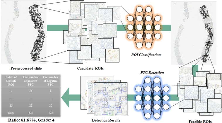
To develop clinically applicable system to identify regions of interest and to detect C4d positive and negative peritubular capillaries in giga-pixel immunostained slides, we proposed and evaluated deep-learning-assisted labeling with more efficiency, enhancing the detection model with pathologists’ insights with enlarged masks, and a fully automated system with combining CNN based classification and detection as routine pathologists’ workflow to predict renal allograft rejection. The overall procedure is described in Fig. 1. The system scans digital images from immunostained pathologic slides and removes background areas by Otsu’s thresholding20. Histogram equalization is processed to reduce variations such as illumination or degree of staining. After selecting all candidate regions of interest (ROIs) with sufficient tissue in each slide, the CNN model classifies ROIs as feasible or non-feasible and detects all C4d positive and negative PTCs in feasible ROIs to determine C4d scores. To train the CNN detection model, enlarged masks with certain sized margins are used as input, so that each enlarged mask includes neighborhood information, such as renal tubules, present near the PTCs. Deep-learning-assisted labeling from independent dataset are used for results determined by the detection model which was trained using dataset by manual labeling. The effectiveness of the enlarged mask and deep-learning-assisted labeling was assessed by comparison with FROC. The CNN detection model using enlarged masks trained with margin sizes of 50 and 40 pixels performed better than those without enlarged masks for the detection of C4d positive and negative PTCs, respectively. In comparisons of deep-learning-assisted labeling, the CNN detection model trained with either or both data by deep-learning-assisted labeling performed better than the model trained with data by manual labeling.
Figure 1.
Overall procedure of our proposed method.
Materials and Methods
The institutional review board for human investigations at Asan Medical Center (AMC) approved the study protocol with removal of all patient identifiers from the images, and waived the requirement for informed consent, in accordance with the retrospective design of this study. A total of 380 needle biopsies of renal allografts were obtained from patients who underwent renal transplantation at AMC from 2009 to 2016; all samples had been stored in the Department of Pathology.
To obtain representative samples, cases in the period were randomly selected without consideration for specific pathologic diagnosis. Consequently, 108 C4d positive and 272 C4d negative cases were retrieved including 46 zero-day allograft biopsies. Two pathologists meticulously reviewed all slides and modified false negative results; finally, 189 cases were classified as C4d positive and 191 cases as C4d negative. C4d was assessed immunohistochemically using a Ventana BenchMark XT autostainer (Ventana Medical Systems, Tucson, AZ, USA), and 380 whole slides were imaged using a digital slide scanner (Pannoramic 250 Flash, 3DHISTECH, Budapest, Hungary) with a 20× objective lens (specimen-level pixel size, 0.221 × 0.221 μm). All samples were anonymized before analysis and labeling.
The 380 slides were divided into subsets 1 and 2, consisting of 200 and 180 slides, respectively, to validate the feasibility of using deep-learning-assisted labeling. Subset 1 was used to train the CNN model for classification and detection, and subset 2 was used to validate the model. The slides in the two subsets were randomized for training (60%), test (20%), and validation (20%). Computational complexity of feasible ROI classification and PTC detection takes constant time. The average time (and standard deviation) for automatic system per slide was 785.81 (±176.97) sec. In this average time, the time for classification per slide and detection per ROI was 712.23 (±132.62) and 0.49 (±0.02) sec where the number of average feasible ROIs was 147.61 (±105.02).
Feasible ROI Classification
All randomly identified candidate ROIs were independently labeled by three pathologists as feasible or non-feasible criteria. Sensitivity was maximized by identifying as many feasible ROIs as possible within each slide. A ROI was classified as non-feasible when more than two-thirds of its image consisted of suboptimal areas, defined as 1) an artifact or poorly stained area that limited proper interpretation; 2) areas without PTCs, such as a large vessel, glomerulus, or vacant area; and 3) scarred or infracted areas21. Examples for criteria are shown in Fig. 2.
Figure 2.
Decision criteria to classify feasible and non-feasible ROIs. (a) Feasible ROI, (b–d) non-feasible ROIs from dominant ambiguous regions including scar, glomerulus, and vessels.
A ROI size of 1024 × 1024 pixels was defined by the pathology team, as an image of this size provided a field of vision similar to a 400 × optical microscopic view, the maximum magnification used in routine practice. The total number of ROIs in subset 1 was 2723, including 2134 feasible and 769 non-feasible ROIs.
The CNN classification model was trained to classify feasible and non-feasible ROIs using an Inception v3 network22 and an ImageNet pre-trained model23. To prevent model overfitting from unbalanced data, adjacent regions were assessed to equalize proportions between classes. Augmentation methods in real time included horizontal and vertical flipping, rotation (0–90°), and zooming in and out (0–10%). The model was implemented in Keras using the Tensorflow with an NVIDIA GTX 1080 Ti GPU, binary-cross entropy loss, stochastic gradient descent optimizer (SGD) with learning rates of 10−5, and dropout with probability of 0.5. The learning rate was reduced to one-tenth per one-third of total epochs 2000 and more detailed parameters are listed in Table 1. Training was terminated at the lowest loss of the test set. The performance of the CNN classification model was evaluated by determining its sensitivity and specificity.
Table 1.
Parameters used for training CNN classification model and CNN detection model.
| Classification model | Detection model | ||
|---|---|---|---|
| Optimizer | SGD | Optimizer | Adam |
| Learning rate | 1e-5 | Learning rate | 1e-5 |
| Weight decay | 1e-6 | Weight decay | 0.0 |
| Epochs | 2000 | Epochs | 150 |
| Momentum | 0.9 | β1, β2 | 0.9, 0.999 |
| Epsilon | 1e-4 | ||
PTC Detection
Three pathologists independently labeled C4d positive and C4d negative PTCs in feasible ROIs of subset 1 by hand drawing using in-house software. After completing these tasks by self, they had a meeting for the discussion of conflicted cases and made a consensus. In addition, pseudo negative PTCs, consisting of non-PTC regions, such as tubules and glomeruli that can be confused with PTCs, were drawn to train the model robustly.
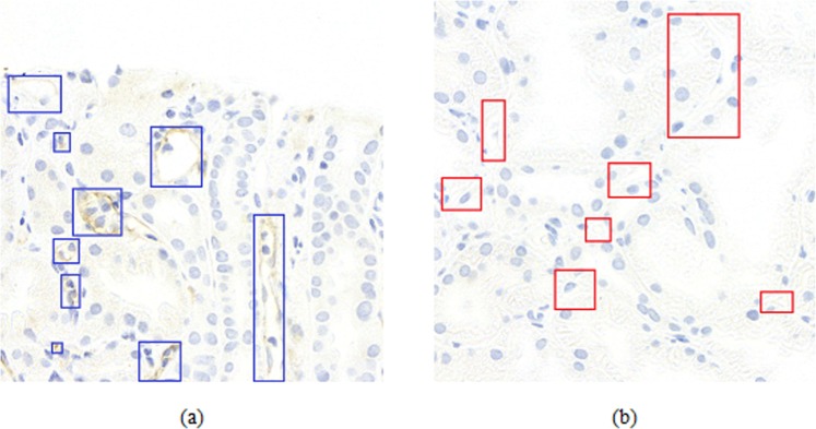
Widths and heights of labeled PTC masks ranged from 25 to 392 pixels. A total of 1823 PTCs were identified by manual labeling, including 549 C4d positive and 1274 C4d negative PTCs, whereas a total of 3836 PTCs were identified from data by deep-learning-assisted labeling, including 1597 C4d positive and 2239 C4d negative PTCs. Examples are shown in Fig. 3.
Figure 3.
Gold standard examples of C4d negative and positive in PTC. Blue and red rectangles show the positive and negative PTC in (a) and (b), respectively.
In general object detection tasks, the object is normally placed on a complex or object-independent background, with object boundaries determined using fitted coordinates. However, pathologic detection of PTCs is different. Because PTCs are capillaries located near tubules, their presence constitutes additional information during training using an enlarged rather than a fitted mask as shown in Fig. 4. An enlarged mask was used because the boundaries of tubules near PTCs could help recognize PTCs on slides. To evaluate the optimal enlarged margin size around manual labeled data, various margin sizes (0–80 pixels at 10-pixel intervals) were adjusted when training the detection model.
Figure 4.
Example of labeled C4d positive PTC with various margin sizes. Margin sizes of (a) 0, (b) 10, (c) 20, (d) 30, (e) 40 pixels.
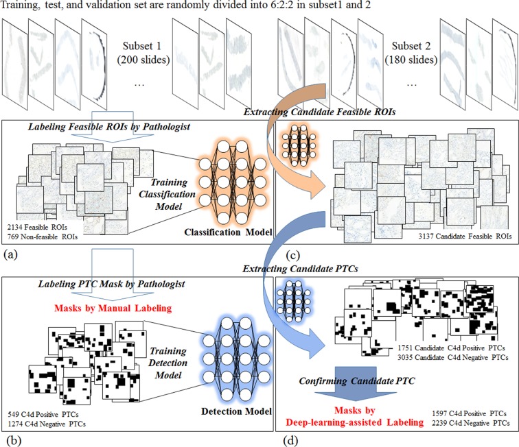
Labeling for massive amounts of data to enhance deep learning performance is time- and labor-intensive. These drawbacks may be overcome by using data by deep-learning-assisted labeling in place of or in addition to manual labeled data. A deep learning model trained for detection can be used to evaluate candidate objects first, followed by confirmation or modification involving little labor to acquire massive data, with the latter called data by deep-learning-assisted labeling. Deep-learning-assisted labeling can reduce the labor required. Figure 5 shows a process used to acquire deep-learning-assisted labeling for detection of C4d positive and negative PTCs. Firstly, two types of CNN model were trained from subset 1 with feasible ROIs and manual labeled mask data (Fig. 5(a,b)). The CNN classification model trained from subset 1 was used to identify feasible ROIs in subset 2 (Fig. 5(c)), and the CNN detection model trained from subset 1 was used to identify candidate C4d positive and negative PTCs in all feasible ROIs. Finally, data by deep-learning-assisted labeling were selected by confirming all candidate PTCs as being C4d positive or C4d negative using an in-house re-labeling tool (Fig. 5(d)). In addition, this procedure was used to test false negative PTCs not detected by the model. If the center of the boundary box identified by the detection model did not deviate significantly from the center of the actual PTC, the PTC was confirmed as C4d positive or negative.
Figure 5.
Sequence for deep-learning-assisted labeling. All slides are randomly divided into 6:2:2 as training, test, and validation set in subset 1 and 2. (a) Training classification model with feasible ROIs in subset 1. (b) Training detection model with manual labeled masks in the feasible ROIs (c). Extracting candidate feasible ROIs in subset 2 by the classification model. (c) Extracting candidate PTCs by the detection model and confirming results of (d) as deep-learning-assisted labeling.
C4d negative and positive PTCs were detected using region proposal based Faster R-CNN detection algorithm4 with ImageNet pre-trained model based Resnet506. Augmentation methods in real time included horizontal and vertical flipping, rotation (0–90°), and zooming in and out (0–10%). The model was implemented in Keras using the Tensorflow with an NVIDIA GTX 1080 Ti GPU. Smooth L1 loss for bounding box regression and categorical-cross entropy loss for classification network in backbone were used. Adam optimizers with learning rates of 10−5 for region proposal and classification network. More detailed parameters are listed in Table 1. Training was terminated at the lowest loss of the test set. Training was terminated at the lowest loss of the test set.
To evaluate the effectiveness of enlarging margins with faster R-CNN detection algorithm and of using data by deep-learning-assisted labeling with faster R-CNN and one-shot based YOLO v2 detection algorithm24, FROC scores, defined as the average sensitivity at seven predefined false positive rates (1/8, 1/4, 1/2, 1, 2, 4, and 8) per ROI, were calculated.
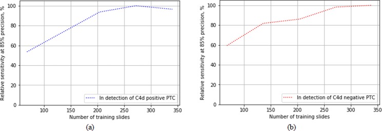
Stress test to see if the 380 slides datasets where the number of positive PTC and negative PTC masks were 2146 and 3513 are sufficient was conducted. To train the different detection CNN model performance with Faster R-CNN for detecting C4d positive and negative PTCs with different amount of training data, all labeled data including subset 1 and subset 2 were used. All data were shuffled and divided into 80% and 20% as training and fixed validation set. Of training set, different training data were randomly selected to train each model at rates of 40%, 60%, 80%, and 100%. Test set for tuning each detection models were randomly selected at rages of 10% in each different training data. To measure performance for detecting C4d positive and negative PTCs, relative sensitivities at as sensitivity were calculated.
Results
Feasible ROI Classification
The CNN classification model trained from subset 1 was tuned with high specificity to minimize false positives. The sensitivity and specificity of the CNN classification model were 0.7951 and 0.9941, respectively.
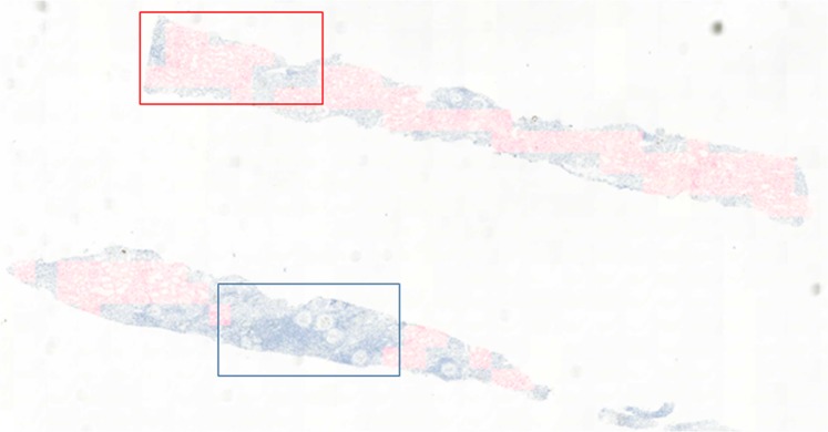
To validate the use of deep-learning-assisted labeling, the CNN classification model trained from subset 1 was used to determine candidate feasible ROIs in subset 2. This model was used to extract feasible ROIs from all tissue regions of subset 2 with high specificity. The mean ± SD number of ROIs per slide was 89.23 ± 34.22. An example of classification results for all regions of a slide is shown in Fig. 6. Tissues containing feasible and non-feasible ROIs were colored red. ROIs containing tubules with PTCs were classified as feasible, whereas ROIs containing scars and glomeruli were classified as non-feasible.
Figure 6.
Feasible and non-feasible ROI classification results. Tissues including feasible ROIs are colored red.
PTC detection
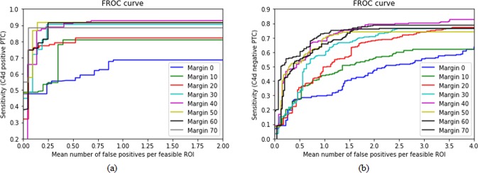
The performances of validations using margin sizes of 0–70 pixels to detect C4d positive and negative PTCs on manual labeled data were compared in Fig. 7 and Table 2 with Faster R-CNN detection algorithm. FROC scores and overall sensitivities for the detection of C4d positive and negative PTCs increased as margin sizes increased. However, overall sensitivities and FROC scores in detecting C4d positive PTCs were optimal at margin sizes of 50 pixels, decreasing at 60 pixels (Fig. 7(a)). Similarly, overall sensitivities and FROC scores in detecting C4d negative PTCs scores were optimal at 40 pixels (Fig. 7(b)). FROC scores were highest for models trained with margin sizes of 50 and 40 pixels for the detection of C4d positive and negative PTCs, respectively.
Figure 7.
FROC comparisons at different size of margin on manual labeled data. Results for detection of (a) C4d positive and (b) negative PTC.
Table 2.
The sensitivities and FROC scores for faster R-CNN detection of C4d positive and negative PTC with various margin sizes (0 to 70) at different mean number of false positives per feasible ROI.
| Mean of FPs | Margin size for detection of C4d positive PTC | |||||||
|---|---|---|---|---|---|---|---|---|
| 0 | 10 | 20 | 30 | 40 | 50 | 60 | 70 | |
| 0.125 | 0.4767 | 0.4862 | 0.7627 | 0.7200 | 0.6575 | 0.8667 | 0.7571 | 0.8851 |
| 0.250 | 0.5397 | 0.5345 | 0.7740 | 0.9045 | 0.8883 | 0.9167 | 0.8136 | 0.8851 |
| 0.500 | 0.5587 | 0.8092 | 0.7910 | 0.9045 | 0.9106 | 0.9167 | 0.9148 | 0.8851 |
| 1.000 | 0.6854 | 0.8092 | 0.8192 | 0.9045 | 0.9274 | 0.9167 | 0.9148 | 0.8851 |
| 2.000 | 0.6854 | 0.8092 | 0.8192 | 0.9045 | 0.9385 | 0.9167 | 0.9148 | 0.8851 |
| 4.000 | 0.6854 | 0.8092 | 0.8192 | 0.9045 | 0.9385 | 0.9167 | 0.9148 | 0.8851 |
| 8.000 | 0.6854 | 0.8092 | 0.8192 | 0.9045 | 0.9385 | 0.9167 | 0.9148 | 0.8851 |
| Score | 0.6166 | 0.7238 | 0.8006 | 0.8781 | 0.8856 | 0.9095 | 0.8778 | 0.8851 |
| 0.125 | 0.0919 | 0.0935 | 0.0976 | 0.1519 | 0.2306 | 0.0944 | 0.0918 | 0.4087 |
| 0.250 | 0.1258 | 0.2019 | 0.1453 | 0.1706 | 0.4663 | 0.4485 | 0.4248 | 0.5549 |
| 0.500 | 0.2733 | 0.2783 | 0.3541 | 0.3200 | 0.5388 | 0.5272 | 0.5465 | 0.5720 |
| 1.000 | 0.2952 | 0.4367 | 0.4978 | 0.5774 | 0.6789 | 0.6969 | 0.6571 | 0.7293 |
| 2.000 | 0.4655 | 0.5553 | 0.6792 | 0.7080 | 0.7920 | 0.7412 | 0.7611 | 0.7876 |
| 4.000 | 0.6217 | 0.6195 | 0.7743 | 0.7633 | 0.8274 | 0.7412 | 0.7633 | 0.7876 |
| 8.000 | 0.7257 | 0.6195 | 0.7743 | 0.7655 | 0.9004 | 0.7412 | 0.7633 | 0.7876 |
| Score | 0.3713 | 0.4006 | 0.4746 | 0.4938 | 0.6334 | 0.5700 | 0.5725 | 0.6611 |
The CNN detection models trained with margins of 40 pixels for the detection of C4d positive and negative PTCs were tuned to maximum sensitivity to generate as much data by deep-learning-assisted labeling as possible. Deep-learning-assisted candidate labeled data were generated by the CNN detection models, which have a recall and precision of 0.8821 and 0.9384, respectively, for the detection of C4d positive PTCs, and of 0.8094 and 0.7108, respectively, for the detection of C4d negative PTCs. The characteristics of manual and deep-learning-assisted labeling differed slightly, in that manual labeled data only included masks fitted to both classes, whereas deep-learning-assisted labeling also included masks that were slightly misplaced locally. Figure 8(a,b) shows inter- and intra-observer variations, respectively, between subset 1 (manual labeling) and subset 2 (deep-learning-assisted labeling). To validate the feasibility of using deep-learning-assisted labeling, FROC scores and sensitivities were compared in models trained with data by manual labeled, data by deep-learning-assisted labeling, and both together at different mean numbers of false positive PTCs per feasible ROI with two different type of detection algorithm. In detecting C4d positive and negative PTCs, the Faster R-CNN model showed better accuracies than those of YOLO v2 model. In addition, both models trained by subset 2 or fusion dataset including subset 1 and subset 2 showed better accuracies (Fig. 8(c,d) and Table 3).
Figure 8.
FROC comparisons for validation of feasibility of using deep-learning-assisted labeling. FROC comparisons to show inter- and intra-observer variation between different validation set for detection of (a) C4d positive and (b) negative PTC with faster R-CNN detection algorithm. FROC comparisons to validate effectiveness of deep-learning-assisted labeling for detection of (c) C4d positive and (d) negative PTC with faster R-CNN and YOLO v2 detection algorithms.
Table 3.
The sensitivities and FROC scores for faster R-CNN and YOLO v2 detections of C4d positive and negative PTC with different detection models trained by different dataset at different mean number of false positives per feasible ROIs (0 to 2 and 0 to 8 for detection of positive and negative PTC, respectively). Model 1: trained by subset 1, Model 2: trained by subset 2, Model 3: trained by fusion of subset 1 and 2.
| Mean of FPs | Detection model for C4d positive PTC | Detection model for C4d negative PTC | ||||
|---|---|---|---|---|---|---|
| Model 1 | Model 2 | Model 3 | Model 1 | Model 2 | Model 3 | |
| Faster R-CNN | ||||||
| 0.125 | 0.6970 | 0.5495 | 0.5768 | 0.1387 | 0.0863 | 0.1148 |
| 0.250 | 0.7803 | 0.6923 | 0.7510 | 0.3333 | 0.1969 | 0.2405 |
| 0.500 | 0.7886 | 0.8791 | 0.8817 | 0.3966 | 0.4579 | 0.4343 |
| 1.000 | 0.9024 | 0.9451 | 0.9253 | 0.5615 | 0.6969 | 0.6644 |
| 2.000 | 0.9187 | 0.9478 | 0.9585 | 0.7082 | 0.8424 | 0.8131 |
| 4.000 | 0.9187 | 0.9478 | 0.9647 | 0.8075 | 0.9294 | 0.8887 |
| 8.000 | 0.9187 | 0.9478 | 0.9647 | 0.8563 | 0.9294 | 0.8910 |
| Score | 0.8463 | 0.8442 | 0.8603 | 0.5431 | 0.5913 | 0.5781 |
| YOLO v2 | ||||||
| 0.125 | 0.3864 | 0.7009 | 0.6736 | 0.0058 | 0.2034 | 0.1928 |
| 0.250 | 0.6284 | 0.7479 | 0.6795 | 0.0032 | 0.3644 | 0.2240 |
| 0.500 | 0.6817 | 0.8333 | 0.7329 | 0.2945 | 0.5512 | 0.4494 |
| 1.000 | 0.7124 | 0.8462 | 0.7567 | 0.5394 | 0.6617 | 0.4761 |
| 2.000 | 0.7221 | 0.8547 | 0.7565 | 0.5423 | 0.7480 | 0.6121 |
| 4.000 | 0.7444 | 0. 8761 | 0.7864 | 0.5423 | 0.8100 | 0.7106 |
| 8.000 | 0.7444 | 0.8846 | 0.7864 | 0.5423 | 0.8100 | 0.7345 |
| Score | 0.6599 | 0.8112 | 0.7388 | 0.3528 | 0.5926 | 0.4856 |
The CNN detection models for detecting C4d positive and negative PTCs trained with different amount of training dataset were compared as shown in Fig. 9. The performances in detection of C4d positive and negative PTC were shown to be saturated at around 300 slides.
Figure 9.
Relative sensitivities comparisons of detection models trained with different amount of training data for detecting (a) C4d positive and (b) negative PTC with faster R-CNN detection algorithm.
Discussion
To develop clinically applicable system, deep-learning-assisted labeling with more efficiency, enhancing the detection model with pathologists’ insights, combining CNN based classification and detection for a fully automated system were developed in this paper. Training the CNN detection models with enlarged masks surrounding PTC region is inspired by the actual pathologists’ insights, which enhanced the detection performance highly (Fig. 7 and Table 2). Deep learning models generally need massive data for training. To overcome the problem of small dataset, we tried to determine a feasibility of deep-learning-assisted labeling that is made from independent dataset with low-labor, which could alleviate massive manual labor. In our experiments, using deep-learning-assisted labeling for training, the performance of the detection model was enhanced (Fig. 8(c,d) and Table 3) compared with only dataset by using manual labeling only, because deep-learning-assisted labeling help draw PTC masks more robustly with less variations such as inter- and/or intra-observer, illumination, and degree of staining. In addition, massive dataset would improve the performance of the CNN detection models. In the stress test, we showed that 380 slides were sufficient to train CNN detection model for finding positive and negative PTC.
Deep learning on pathologic images could depend on various scanning conditions such as not only illumination, but also the degree of staining, different equipment, and so on. To overcome these problems, pre-trained network which has been already trained with bunch of tremendous number of images having a variety of complex variation, histogram normalization that is one of stain normalization method, and doubled dataset by deep-learning-assisted labeling were used to train our deep learning model to have robustness of them.
The most important aspects of application of this system to pathology are full automation for objective diagnosis and alleviation of manual labor. This study proposed a fully automated two-step CNN system for the diagnosis of allograft rejection. The first step consists of the use of a CNN classification model to identify feasible ROIs in all tissue regions and the second step consists of the use of a CNN detection model to identify and count C4d positive and negative PTCs, a marker of allograft rejection in kidney transplant recipients. These findings suggest that this system may be applicable to most tasks in digital pathology.
Classification of all tissue regions as feasible or non-feasible ROIs using the CNN classification model is practical, as pathologists cannot determine all feasible ROIs in a tissue sample and have difficulty identifying negative PTCs. By contrast, the CNN classification model can precisely evaluate the entire specimen, and the CNN detection model can accurately count the numbers of C4d positive and negative PTCs in all feasible ROIs. Determining both C4d positive and C4d negative PTCs may alter clinical diagnoses.
In addition, two kinds of performance comparisons were conducted. Firstly, the performances of models trained with different size of margin including PTC region were compared. Enlarged mask with a certain size improved detection CNN model, which method was mimicked by a real clinical experience. This novelty including surrounding regions could be used widely for similar tasks. Secondly, the performances of models trained with data by manual labeling and data by deep-learning-assisted labeling were compared. The generation of data by deep-learning-assisted labeling and confirmation by expert pathologists may help improve the performance of these models. Pathologic labeling is very difficult, even for expert pathologists, whereas the deep-learning-assisted method generated relatively robust labels.
Several obstacles should be overcome before clinical application. The sample size (380 slides) is about 1.2 times the average renal allograft biopsy per year in this center, which is one of the largest medical center in South Korea. Though it is also relatively larger than other studies related to pathologic assessment using convolutional neural network9,11,12, we will try to evaluate the performance of this more with wild dataset from larger data. Also, all cases were recruited from a single center using only one slide scanner, which could lead to less variations such as background illumination or degree of staining. To evaluate the robustness of this method, further studies with multi-center could be needed. In addition, comparisons of the performance and outcomes of this method with those of pathologists are needed to determine the clinical effectiveness of this system.
Conclusion
Pathologic examination is time-consuming, involving the examination of all areas of cells using a digital microscope. Subjectively determined pathologic diagnoses may differ and may be easily susceptible to inter- and/or intra-observer variations. These drawbacks may be overcome by an automatic method of PTC scoring using two types of trained models (window classification and PTC detection). Classification, detection, and scoring comparisons showed that this method yielded reasonable results when evaluating stained giga-pixel digital slides. Use of this system may be feasible diagnostically in detecting other diseases and conditions.
Acknowledgements
This work was supported by Kakao and Kakao Brain corporations, and a Grant (2017-7028) from the Asan Institute for Life Sciences, Asan Medical Center, Seoul, Korea.
Author Contributions
Y.-G.K. and N.K. wrote the main manuscript text. Y.-G.K., Y.C. and H.L. performed experiments and prepared figures. A-R.L. and B.P., wrote the Java and Python codes for labeling tools. G.C. and H.G. prepared the datasets. All authors reviewed the manuscript.
Competing Interests
The authors declare no competing interests.
Footnotes
Publisher’s note: Springer Nature remains neutral with regard to jurisdictional claims in published maps and institutional affiliations.
Young-Gon Kim and Gyuheon Choi contributed equally.
Contributor Information
Heounjeong Go, Email: damul37@naver.com.
Namkug Kim, Email: namkugkim@gmail.com.
References
- 1.Krizhevsky, A., Sutskever, I. & Hinton, G. E. Imagenet classification with deep convolutional neural networks. Advances in neural information processing systems, 1097–1105 (2012).
- 2.Szegedy C, Ioffe S, Vanhoucke V, Alemi AA. Inception-v4, inception-resnet and the impact of residual connections on learning. AAAI. 2017;4:12. [Google Scholar]
- 3.Liu, W. et al. Single shot multibox detector. European conference on computer vision, 21–37 (2016).
- 4.Ren, S., He, K., Girshick, R. & Sun, J. Faster r-cnn: Towards real-time object detection with region proposal networks. Advances in neural information processing systems, 91–99 (2015). [DOI] [PubMed]
- 5.Long, J., Shelhamer, E. & Darrell, T. Fully convolutional networks for semantic segmentation. Proceedings of the IEEE conference on computer vision and pattern recognition. 3431–3440 (2015). [DOI] [PubMed]
- 6.He, K., Zhang, X., Ren, S. & Sun, J. Deep residual learning for image recognition. Proceedings of the IEEE conference on computer vision and pattern recognition. 770–778 (2016).
- 7.Gulshan V, et al. Development and Validation of a Deep Learning Algorithm for Detection of Diabetic Retinopathy in Retinal Fundus Photographs. JAMA. 2016;316:2402–2410. doi: 10.1001/jama.2016.17216. [DOI] [PubMed] [Google Scholar]
- 8.Esteva A, et al. Dermatologist-level classification of skin cancer with deep neural networks. Nature. 2017;542:115–118. doi: 10.1038/nature21056. [DOI] [PMC free article] [PubMed] [Google Scholar]
- 9.Bejnordi BE, et al. Diagnostic assessment of deep learning algorithms for detection of lymph node metastases in women with breast cancer. JAMA. 2017;318:2199–2210. doi: 10.1001/jama.2017.14585. [DOI] [PMC free article] [PubMed] [Google Scholar]
- 10.Golden JA. Deep Learning Algorithms for Detection of Lymph Node Metastases From Breast Cancer: Helping Artificial Intelligence Be Seen. JAMA. 2017;318:2184–2186. doi: 10.1001/jama.2017.14580. [DOI] [PubMed] [Google Scholar]
- 11.Araujo, T. et al. Classification of breast cancer histology images using Convolutional Neural Networks. Plos One12, doi:ARTN e017754410.1371/journal.pone.0177544 (2017). [DOI] [PMC free article] [PubMed]
- 12.Arvaniti, E. et al. Automated Gleason grading of prostate cancer tissue microarrays via deep learning. bioRxiv, 280024 (2018). [DOI] [PMC free article] [PubMed]
- 13.Xu Y, et al. Large scale tissue histopathology image classification, segmentation, and visualization via deep convolutional activation features. BMC Bioinformatics. 2017;18:281. doi: 10.1186/s12859-017-1685-x. [DOI] [PMC free article] [PubMed] [Google Scholar]
- 14.Behrmann J, et al. Deep learning for tumor classification in imaging mass spectrometry. Bioinformatics. 2018;34:1215–1223. doi: 10.1093/bioinformatics/btx724. [DOI] [PubMed] [Google Scholar]
- 15.Regele H, et al. Capillary deposition of complement split product C4d in renal allografts is associated with basement membrane injury in peritubular and glomerular capillaries: a contribution of humoral immunity to chronic allograft rejection. Journal of the American Society of Nephrology. 2002;13:2371–2380. doi: 10.1097/01.ASN.0000025780.03790.0F. [DOI] [PubMed] [Google Scholar]
- 16.Haas M, et al. The Banff 2017 Kidney Meeting Report: Revised diagnostic criteria for chronic active T cell–mediated rejection, antibody‐mediated rejection, and prospects for integrative endpoints for next‐generation clinical trials. American Journal of Transplantation. 2018;18:293–307. doi: 10.1111/ajt.14625. [DOI] [PMC free article] [PubMed] [Google Scholar]
- 17.Gibson I, et al. Peritubular capillaritis in renal allografts: prevalence, scoring system, reproducibility and clinicopathological correlates. American Journal of Transplantation. 2008;8:819–825. doi: 10.1111/j.1600-6143.2007.02137.x. [DOI] [PubMed] [Google Scholar]
- 18.Mengel M, et al. Banff initiative for quality assurance in transplantation (BIFQUIT): reproducibility of C4d immunohistochemistry in kidney allografts. American Journal of Transplantation. 2013;13:1235–1245. doi: 10.1111/ajt.12193. [DOI] [PubMed] [Google Scholar]
- 19.Brazdziute, E. & Laurinavicius, A. Digital pathology evaluation of complement C4d component deposition in the kidney allograft biopsies is a useful tool to improve reproducibility of the scoring. Diagnostic pathology. S5 (BioMed Central). [DOI] [PMC free article] [PubMed]
- 20.Otsu N. A threshold selection method from gray-level histograms. IEEE transactions on systems, man, and cybernetics. 1979;9:62–66. doi: 10.1109/TSMC.1979.4310076. [DOI] [Google Scholar]
- 21.Racusen LC, Halloran PF, Solez K. Banff 2003 meeting report: new diagnostic insights and standards. American journal of transplantation. 2004;4:1562–1566. doi: 10.1111/j.1600-6143.2004.00585.x. [DOI] [PubMed] [Google Scholar]
- 22.Szegedy, C., Vanhoucke, V., Ioffe, S., Shlens, J. & Wojna, Z. Rethinking the inception architecture for computer vision. CVPR, 2818–2826 (2016).
- 23.Deng, J. et al. Imagenet: A large-scale hierarchical image database. CVPR, 248–255 (2009).
- 24.Redmon, J. & Farhadi, A. YOLO9000: better, faster, stronger. https://arxiv.org/abs/1612.08242 (2017).


