Representing GHG Reduction Technologies in the Future Fleet with Full Vehicle Simulation

Abstract

As part of an ongoing assessment of the potential for reducing greenhouse gas emissions of light-duty vehicles, the U.S. Environmental Protection Agency (EPA) has implemented an updated methodology for applying the results of full vehicle simulations to the range of vehicles across the entire fleet. The key elements of the updated methodology explored for this paper, responsive to stakeholder input on the EPA’s fleet compliance modeling, include 1) greater transparency in the process used to determine technology effectiveness, and 2) a more direct incorporation of full vehicle simulation results.

This paper begins with a summary of the methodology for representing existing technology implementations in the baseline fleet using EPA’s Advanced Light‐duty Powertrain (ALPHA) full vehicle simulation. To characterize future technologies, a full factorial ALPHA simulation of every conventional technology combination to be considered was conducted. The vehicle simulation results were used to automatically generate response surface equations (RSEs), enabling the use of a quick and easily implemented set of specific equations to estimate fleet-wide emissions in place of running time consuming full vehicle simulations for each potential technology package applied to each model in the fleet. Since the regressions were not extended to represent technology combinations that were not actually simulated, the emissions estimates produced from the RSEs match the ALPHA simulation results with a high degree of conformity.

For each vehicle in the fleet, the reduction in emissions for a future technology package can be estimated using RSEs associated with the initial and final technology packages, and considering the particular vehicle’s weight, road load, and power. As part of the effectiveness assessment based on weight, road load, and power, this paper will also examine the effect of performance changes in the vehicles.

Introduction

In previous assessments of technology for greenhouse gas (GHG) emissions reduction, the U.S. Environmental Protection Agency (EPA) had utilized a lumped parameter model (LPM) to determine the “effectiveness” of technology packages, defined as the percentage reduction in CO₂ emissions expected from each package, compared to a constant starting point. [1] In public comments, some industry stakeholders have suggested that replacing the LPM with a process more directly tied to full vehicle simulation would result in a more robust analysis of potential CO₂ reduction. This paper describes the approach that has been implemented by the EPA to expand and more directly apply full vehicle simulation in its overall modeling methodology.

The LPM used in past assessments relied on a manual calibration process, and the tie between the ALPHA full-vehicle simulation and the resulting LPM assignments of technology effectiveness was indirect. To improve the transparency and reduce the effort involved with that process, EPA has eliminated the manual calibration of effectiveness values and is now utilizing vehicle-class-specific response surface equations (RSEs) automatically generated from a large number of ALPHA runs. This change in methodology will allow the EPA to more readily utilize large-scale simulation results, while at the same time providing the engineering community at large an easily accessible and usable tool to explore EPA’s ALPHA simulations, and/or produce their own RSEs for comparison based on their own large-scale simulation results.

Modeling Current Technology Packages

The process of assessing the potential for CO₂ reduction begins with analysis and modeling of each vehicle in the current baseline fleet. For this analysis, EPA chose the 2016 model year (MY2016) fleet, which at the time of this writing was the latest available with both verified production volume data and vehicle technology configuration parameters. Specific test weights, road loads, engine sizes, and actual measured CO₂ emissions values over the city (Federal Test Procedure, or FTP) and highway (HW) cycles were available for each of the vehicles in the baseline fleet.

For each vehicle in the baseline fleet, the powertrain was characterized using a representative technology package chosen from EPA’s library of benchmarked engine, transmission, accessory and hybridization models. Each baseline vehicle was individually modeled with an ALPHA full vehicle simulation to verify the technology package detail. More detail on this methodology is presented in reference. [2]

Vehicle Effectiveness Classes and Exemplar Vehicles

Using the baseline fleet vehicle characteristics, six vehicle “effectiveness classes” were determined, grouping vehicles with similar characteristics for the purposes of determining technology effectiveness. These effectiveness classes divide the fleet according to engine power and vehicle loads. The total vehicle load is composed of both inertial load (represented by the vehicle’s equivalent test weight, or ETW) and road loads (primarily tire rolling and aerodynamic loading), which are only loosely correlated. Therefore, the vehicle loads were defined two-dimensionally, using both power-to-weight ratio (P/W ratio) and road load horsepower at 50 mph (22.4 m/sec), notated in this paper as RLHP@50. (Note that within US emission and certification procedures, vehicle characteristic values are recorded in English units rather than SI units. As the following analysis is substantially based on these characteristic values, this paper will use English units preferentially.)

First, all vehicles that are body-on-frame trucks were separated into their own class. These vehicles, with a high capacity for towing and hauling, have road loads that tend to be substantially higher than other passenger vehicles. This “truck” class accounts for 16.6% of the vehicle production volume of the MY2016 fleet.

The remaining vehicles were categorized into low, medium, and high P/W ratio levels based on actual production volumes of the MY2016 production fleet. Vehicles in the lowest 40% of P/W ratio, by production volume, were assigned to the “low” P/W level; vehicles within the 40% to 80% range were assigned to the “mid” P/W ratio level, and vehicles with the highest 20% P/W ratio were assigned to the “high” P/W ratio level. The range of P/W ratio values for each level, as well as those for the “truck” class, are shown in Figure 1 as cumulative fractions of the production volume. The production volumes for plug-in vehicles (plug-in hybrid electric vehicles [PHEVs] and battery electric vehicles [BEVs]) were not included in the percentile calculations for power-to-weight ratios. These vehicles make up less than 1% of the production-weighted vehicle production volume in MY2016.

Figure 1.

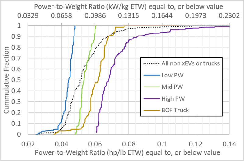
Production volume distribution of P/W ratios in the MY2016 fleet. BEVs and PHEVs are not included in the analysis, and body-on-frame trucks are seperated from the remainder of the fleet.

For the next step, the distribution of RLHP@50 values was calculated for each of the P/W ratio categories. The result for each category is shown in Figure 2 as the cumulative fraction of the production volume.

Figure 2.

Production volume distribution of RLHP@50 in the MY2016 fleet. BEVs and PHEVs are not included in the analysis, and body-on-frame trucks are seperated from the remainder of the fleet. The remaining vehicles have been seperated according to their P/W ratio classification. Class cutoff points between high and low RLHP@50 values are noted.

Both the low and mid P/W ratio categories exhibit somewhat bimodal distributions, with vehicles clustered in two groups below and above the category’s median value of road load horsepower. Generally, the vehicles within these two groups tend to correspond to cars (with lower road loads) and sport-utility vehicles and vans (with higher road loads). In recognition of the relatively broad and bimodal distributions of road load horsepower, the low and mid P/W ratio categories were further subdivided into “low” and “high” RLHP@50 levels as shown in Table 1, using the cutoff values marked in Figure 2.

Table 1.

Criteria for classifying vehicles by P/W ratio and RLHP@50. The cutoff values shown can be inferred from the distributions shown in Figures 1 and 2.

P/W ratio				RLHP@50 mph (22.4m/s)
Level	% Range	Cutoff values HP/lb ETW (kW/kg ETW)		Level	% Range	Cutoff values HP (kW)
Low	0–41	-	0.048 (0.082)	Low	0–54	-	12.3 (9.2)
				High	54–100	12.3 (9.2)	-
Mid	41–80	0.048 (0.082)	0.061 (0.104)	Low	0–45	-	12.6 (9.4)
				High	45–100	12.6 (9.4)	-
High	80–100	0.061 (0.104)	-	-	-	-	-

The result of this process is the construction of six effectiveness classes, with all non-plug-in MY2016 vehicles assigned to one of the classes. The final distribution of the fleet among the six classes, as a function of P/W ratio and RLHP@50, is shown in Figure 3.

Figure 3.

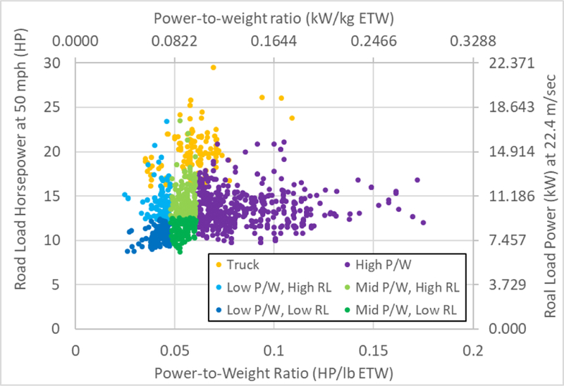
Distribution of the MY2016 fleet vehicles, by P/W ratio and RLHP@50. Dots are for individual vehicles and are not production-weighted.

For each effectiveness class, an “exemplar” vehicle was defined, using the production-weighted average characteristics of the vehicles within the class. The values for engine power, vehicle coastdown coefficients, and ETW are given in Table 2, based on the MY2016 fleet.

Table 2.

Characteristics of exemplar vehicles for the six effectiveness classes. The effectiveness class name reflects the range of power/weight ratio and RLHP@50 values from Table 1. Values represent the production-weighted averages of each parameter for the vehicles within the class.

Effectiveness Class	Engine HP (kW)	A coeff lbf (N)	B coeff lbf/mph (N/mps)	C coeff lbf/mph2 (N/mps2)	ETW lbs (kg)
Low P/W, Low RL	142.5 (106.3)	26.56 (117.9)	0.1067 (1.0595)	0.01858 (0.4129)	3287 (1491)
Mid P/W, Low RL	184.5 (137.6)	31.16 (138.3)	−0.0320 (−0.3183)	0.01991 (0.4424)	3510 (1595)
High P/W	309.4 (230.7)	35.53 (157.7)	0.2822 (2.8027)	0.02152 (0.4782)	4293 (1947)
Low P/W, High RL	168.2 (125.4)	32.91 (146.1)	0.1810 (1.7981)	0.02437 (0.5415)	3836 (1740)
Mid P/W, High RL	249.6 (186.1)	39.00 (173.2)	0.1642 (1.6313)	0.02598 (0.5772)	4474 (2029)
Truck	325.1 (242.4)	39.17 (173.9)	0.4138 (4.1107)	0.03348 (0.7440)	5336 (2420)

Modeling Vehicle Technology Packages in ALPHA

Each of the six nominal exemplar vehicles was modeled using the ALPHA tool. ALPHA is a physics‐based, forward‐looking, full vehicle computer simulation capable of analyzing various vehicle types combined with different powertrain technologies and evaluating the synergistic effects of the individual powertrain and load reducing technologies to improve fuel economy and reduce CO₂. The software tool is a MATLAB/Simulink based application. [3]

To each vehicle, a matrix of combinations of technology were applied. Four different technology areas were considered within vehicle technology packages for this analysis. These were engines, transmissions, mild electrification technologies, and the reduction of vehicle loading.

For vehicle engines, eight different engine maps were used in the vehicle simulations for each exemplar vehicle (for three of these eight, one of two similar engines was chosen, depending on the effectiveness class). The eight engines were:

1. NA GDI engine based on either a 4.3L GM EcoTec engine from a 2014 Silverado, without cylinder deactivation, [4] or a 2.5L GM EcoTec engine from a 2014 Chevrolet Malibu [5]

2. NA PFI engine based on either the 2.5L GM EcoTec engine or the 4.3L GM EcoTec engine, with a PFI conversion adapted from Ricardo study modeling results. [6]

3. NA Atkinson engine based on a 2.0L Mazda engine from a 2014 Mazda 3. [7]

4. NA Atkinson engine based on the 2.0L Mazda engine, with the addition of cooled EGR and cylinder deactivation. [8]

5. NA Atkinson engine based on a 2.5L Toyota engine from a 2018 Toyota Camry. [9]

6. Turbocharged engine based on either a 1.6L Ford EcoBoost engine from a 2013 Ford Escape [10] or a 2.7L Ford EcoBoost engine from a 2015 Ford F150. [11]

7. Turbocharged engine based on a 1.5L Honda engine from a 2017 Honda Civic. [12]

8. 24-bar turbocharged engine based on Ricardo study modeling results. [13]

Additionally, the effect of cylinder deactivation was applied to four of these engine maps. These four were the NA GDI engine, the NA PFI engine, the turbocharged Honda engine, and the turbocharged Ford EcoBoost engine. The effect of cylinder deactivation was modeled in two ways:

1. A discrete number of cylinders were deactivated, similar to the strategy employed on the 4.3L GM EcoTec engine. [4]

2. A variable number of cylinders were deactivated in a continuous manner, similar to the strategy employed in the Tula Dynamic Skip Fire system. [14, 15]

The final result was 16 separate engine maps: eight without cylinder deactivation, and four each with the discrete and variable cylinder deactivation varieties.

For vehicle transmissions, five different transmission maps were used in the vehicle simulations:

1. A five-speed transmission based on a 2007 Toyota Camry transmission and adapted from Ricardo study modeling results. [18]

2. A six-speed transmission based on the GM 6T40. [5]

3. An eight-speed transmission based on the FCA 845RE. [16]

4. An eight-speed transmission based on ZF’s projected potential improvements in future transmissions, along with advanced warmup and control strategies. [17]

5. A six-speed transmission based on the GM 6T40, with improvements similar to the eight-speed. [5, 17]

For mild electrification technologies, three levels were modeled: no electrification, stop/start only, and a mild 48V hybrid system. The stop/start package applied in the simulations shut the engine off when the vehicle came to a stop, and then restarted the engine approximately when the driver’s foot would be removed from the brake pedal. The engine-shutoff feature was disabled until 100 seconds after a cold start to account for engine-warmup strategies.

The 48V mild hybrid system was modeled as a belt integrated starter generator (BISG) P0 48V mild hybrid parallel hybrid electric system with rule-based vehicle supervisory controls which identify overall energy flows by controlling key parameters like state of charge, pedal acceleration/deceleration, vehicle speed, battery power limits, and the demanded driver torque. A full description of this control system is included in reference [19].

For changes to vehicle loading, reductions in rolling resistance, aerodynamic resistance, and vehicle weight were considered, at values of 0%, 10%, and 20% reduction from the baseline values for each load.

The combination of these areas resulted in (16 engines) × (5 transmissions) × (3 mild electrification levels) × (3 levels of rolling resistance) × (3 levels of aero resistance) × (3 levels of weight reduction) = 6840 distinct combinations of technology. A full factorial set of ALPHA simulations was performed to calculate the amount of CO₂ produced from each tech package for each exemplar vehicle.

Each vehicle simulated in the matrix was assumed to have electric power steering and a high efficiency alternator. In addition, the combination of a PFI engine, five-speed transmission, hydraulic power steering (opposed to electric power steering) and no additional technology was simulated. This package was considered a “null vehicle” package to which all the other packages were compared.

The technologies described in this paper represent the state of the analysis at the time of this writing. EPA continuously evaluates the most recent information available on technological improvements to inform its estimate of the potential for GHG reduction in the future fleet. New technologies may be incorporated into this analysis as they are developed, and the representation of technologies may change as new information becomes available.

Performance and Engine Sizing

For each of the exemplar vehicles, a nominal powertrain package was defined, consisting of the NA GDI engine and the 6-speed automatic transmission. [20] For modeling purposes, the engine map was resized to match the peak power of each exemplar vehicle (given in Table 2). As part of the resizing process, the engine’s BSFC was adjusted using scaling rules that accounted for changes in heat transfer, FMEP, and knock sensitivity. Transmission and torque converter losses were also modified to account for scaling. [21]

For the remainder of ALPHA simulation runs, the acceleration performance of each vehicle package was matched to that of the nominal powertrain package by appropriately resizing the engine. EPA has chosen to maintain consistent acceleration performance for ALPHA fleet modeling so that the relative cost-effectiveness of the technologies can be fairly compared, and the effects of CO₂ reduction technologies on vehicle performance are not unduly ignored. [1, 22]

The acceleration performance to be matched was defined as the sum of four acceleration times: 0–60 mph (0–26.8 m/s) time, ¼ mile (402 m) time, 30–50 mph (13.4–22.4 m/h) passing time, and 50–70 mph (22.4–31.3 m/h) passing time for the exemplar vehicle containing the nominal powertrain package. These four metrics were chosen to give a reasonably broad set of acceleration metrics that would be sensitive enough to represent true acceleration performance, but not so sensitive that minor changes in vehicle parameters would significantly change the final metric.

Although the absolute magnitude of these four acceleration metrics can be quite different, the change in each metric due to engine resizing is much more consistent. For example, as shown in Figure 4, the ¼-mile time is much greater than the other acceleration metrics, and thus dominates the actual magnitude of the summed acceleration metric. However, as shown in Figure 5, the increase in ¼-mile time with decreasing engine power is roughly the same as the increase in 0–60 time, and only somewhat larger than the change due to the two passing times.

Figure 4.

Calculated acceleration performance times from ALPHA simulation for a medium P/W ratio vehicle over a range of engine horsepowers. This figure is for a GDI engine with six-speed transmission.

Figure 5.

The change in calculated acceleration performance times from the ALPHA simulations in Figure 4, using the largest engine size as a base. These data are the same as shown in Figure 4.

Thus, although the ¼-mile time dominates the magnitude of the summed acceleration metric, the impact of the ¼-mile time on engine sizing is effectively equivalent to that of the 0–60 acceleration time.

To choose the proper engine size to maintain acceleration performance, ALPHA simulations were run with the engine size swept in increments of approximately 2%. The losses in the remaining components of the powertrain, including the transmission, torque converter, and rear end ratio, were sized according to the process laid out in earlier work. [21] The entire vehicle technology package was then run through an ALPHA simulation which calculated the summed acceleration time metric. The engine size steps of approximately 2% lead to vehicle performance times in steps of approximately 1% - 1.5%.

From this series of runs, the engine size resulting in acceleration performance closest to, but no worse than, the acceleration performance of the nominal powertrain package was chosen. The CO₂ emissions over the FTP and HW cycle simulated for that engine size and technology package were then used in further calculations of exemplar effectiveness. Because of the increments used in powertrain sizing, the final CO₂ emissions within the simulations could vary up to around 0.5% from a perfectly performance-neutral number.

Determination of Response Surface Equations

From the performance neutral ALPHA results of the full factorial simulations, a response surface equation (RSE) was generated for each engine technology used in each exemplar vehicle. EPA used the industry standard statistical software JMP from SAS [23] to create the response surface equations. An example RSE is given below for a Med P/W Low RL vehicle with a GDI engine:

CO₂ (g/mile) = 265.80 – 151.97×Mass – 48.81×Aero – 48.57×Roll – 14.103×Trans – 10.475×SS – 1.977×Deac – 7.316×Mass×Aero + 40.886×Mass×Roll + 7.698×Aero×Roll + 2.910×Mass×Trans – 0.2065×Aero×Trans + 0.3171×Roll×Trans + 5.712×Mass×SS + 0.2254×Aero×SS + 0.01754×Roll×SS + 1.1775×Trans×SS + 4.537×Mass×Deac – 1.0453×Aero×Deac – 0.5556×Roll×Deac + 0.46152×Trans×Deac + 0.02507×SS×Deac – 34.15×Mass² + 0×Aero² + 0×Roll² + 1.0690×Trans² + 0×SS² – 2.513×Deac²

The inputs to each RSE include a level of mass reduction (“Mass” in the equation above), level of aerodynamic drag reduction (“Aero”), level of rolling resistance reduction (“Roll”), presence of mild hybridization technology (“SS”, or start-stop), transmission type (“Trans”), and the presence of cylinder deactivation (“Deac”). Mass and road load reductions are represented in the RSE as percentages. Mild hybridization, transmission type, and cylinder deactivation are specified with whole numbers. This allows these discrete technologies to be treated numerically in the RSE in a similar way as technologies that can be applied continuously, such as mass or road load reductions. Using these inputs, RSEs are generated for each engine technology used in each exemplar vehicle.

Throughout this process to determine the equations, the results directly from ALPHA are compared to the results determined from the RSE, as shown in Figure 6, to ensure the validity of the data transfer from ALPHA and RSE equation implementation. An added benefit of this comparison is the verification that the ALPHA model results are smooth and predictable as expected. This type of representation aids the quality control process, and assures a more robust and transparent set of equations as the end result.

Figure 6.

RSE CO₂ values versus the full vehicle simulation results from ALPHA. The RMS difference is under 0.3 g/mile.

For all RSEs in this analysis, the root mean square (RMS) difference between the RSE value and the corresponding ALPHA simulation value was under 0.3 g/mile, with no individual result deviating more than 0.8 g/mile between the RSE and ALPHA values.

Using RSEs for Individual Vehicles in the Fleet

The RSEs for each effectiveness class exemplar can be used to easily determine the expected CO₂ emissions for the exemplar vehicle when it is outfitted with the specified technology package. The percentage difference in emissions between the specified technology package and the “null” package (i.e., a PFI engine and five-speed transmission with no additional technology) represents the “effectiveness” of the package. This effectiveness percentage can then be applied to all vehicles within the effectiveness class to determine the effectiveness of the vehicle within the MY2016 fleet (compared to the null package) and the effectiveness of potential future packages, with different technologies.

One advantage of using multiple response surfaces is that the effectiveness values for individual technologies can vary, depending on the vehicle package. This is particularly true of engines and transmissions, where the individual effectiveness of (for example) an engine is heavily dependent on the transmission which it is coupled with. As an example, Figure 7 shows the effectiveness associated with a specific turbocharged, downsized engine (based on a 2.7L Ford EcoBoost engine) over a PFI engine. In this case, the engine effectiveness ranges from about 7% to over 14%, depending on the transmission and road load adjustments of the base package.

Figure 7.

Calculated effectiveness for implementing a turbocharged engine (based on a 2.7L Ford EcoBoost) in place of a PFI engine, for a range of starting packages. Packages have different transmissions and road load reductions.

The effectiveness of a specific technology will also depend on the effectiveness class to which it belongs. For example, Table 3 shows the effectiveness for two pairs of technology packages. The first pair contains a six speed transmission along with either a GDI engine with variable continuous cylinder deactivation [14, 15] or an Atkinson engine. [9] The second pair contains a GDI engine, six speed transmission, and either 10% mass reduction or 15% reduction of both aerodynamic and rolling resistance.

Table 3.

Technology effectiveness as a function of effectiveness class for two pairs of technology packages: a GDI engine versus an Atkinson engine, and 10% mass reduction versus 15% aerodynamic and 15% rolling resistance reduction.

Effectiveness Class	P/W ratio HP/lb (kW/kg)	RLHP@50 HP (kW)	Six speed transmission +		GDI engine + six speed transmission +
			GDI engine w/ cont. deac	Atkinson engine	10% mass reduction	15% aero + 15% roll reduction
Low P/W, Low RL	0.0434 (0.0713)	10.45 (7.79)	9.8%	13.8%	12.3%	12.3%
Mid P/W, Low RL	0.0526 (0.0864)	10.58 (7.89)	10.1%	10.9%	11.3%	11.0%
High P/W	0.0721 (0.1185)	13.79 (10.28)	11.6%	8.9%	10.4%	8.5%
Low P/W, High RL	0.0438 (0.0721)	13.72 (10.23)	8.5%	12.7%	10.8%	11.5%
Mid P/W, High RL	0.0558 (0.0917)	14.95 (11.15)	10.1%	9.4%	10.1%	9.4%
Truck	0.0609 (0.1002)	19.14 (14.27)	12.3%	13.1%	12.1%	12.4%

Each technology package has near 11% effectiveness, on average, but the individual effectiveness classes have varying effectiveness. In the first pair, the difference in effectiveness is generally a function of the P/W ratio. For the two effectiveness classes with low P/W ratios, the Atkinson engine is considerably more effective than the deac engine. Conversely, for the High P/W class, the Atkinson engine is considerably less effective than the deac engine. This indicates that the power/weight ratio of the vehicle plays a part in selecting the most effective technology package.

In the second pair, the difference in effectiveness is a function of both the P/W ratio and the magnitude of the RLHP@50. In this case, mass reduction tends to be more effective than rolling and aero reduction for higher P/W ratios, and less effective for high RLHP@50. For example, in the High P/W class, the 10% mass reduction is much more effective than the aero and rolling reduction, while in the two low P/W classes, the 10% mass reduction is the same or less effective than the aero and rolling reduction. At the same time, in the Truck class, with its high RLHP@50, the 10% mass reduction is slightly less effective than the aero and rolling reduction despite the high P/W ratio.

As discussed earlier in the paper, the effectiveness classes were defined using vehicle P/W ratios and road loads. The effectiveness class exemplar used for the ALPHA simulations is specified to have nominally average power, weight, and road load coefficients. Thus, the effectiveness which results from adding a technology package to the nominal exemplar vehicle should be reasonably representative of the effectiveness of adding that same technology to all vehicles within the vehicle class.

Effectiveness Adjustment Factors for Engine Power, Vehicle Weight, and Road Load

Although the RSE effectiveness calculated using the exemplar vehicle could be reasonably applied to any vehicle in that effectiveness class, its actual effectiveness value can vary as a function of the vehicle’s engine P/W ratio and RLHP@50 values. To account for this, effectiveness adjustment factors for each effectiveness class were determined using a series of ALPHA simulations with varying engine power and vehicle loads. Vehicle road loads (represented by RLHP@50) are correlated with weight, albeit loosely, as shown in the top graph in Figure 8, where the two parameters are normalized with respect to engine power. To represent the effect of vehicle road loads more independently, the ETW to RLHP@50 ratio was used along with the ETW/engine power (W/P) ratio to characterize the total vehicle loading (see the bottom portion of Figure 8). The W/P ratio was used preferentially in this step (rather that P/W ratio) as the correlations are more linear.

Figure 8.

ETW/engine power ratio versus both RLHP@50/power (top) and ETW/RLHP@50 (bottom) for the MY2016 fleet. As expected, the top graph shows a loose correlation between weight and RLHP@50.

For each exemplar vehicle, a matrix of W/P and ETW/RLHP@50 ratios was created which spanned most of the values for the vehicles represented by that exemplar (see Figure 3). These matrices were created by altering both engine power and road load coefficients in even increments from the base values, while fixing the ETW. ALPHA simulations were run for each set of altered parameters, using the same combinations of technology detailed above.

As an example, the resulting CO₂ values for a null powertrain (PFI engine and five-speed transmission) in a Mid P/W, Low RL exemplar vehicle are shown in Figure 9 as a function of W/P ratio and ETW/RLHP@50 ratios. Note that the magnitude of the CO₂ results depends on the absolute values of ETW, engine power, and road loads, and not merely the ratios of these values. To be more representative, the same CO₂ values are also shown normalized by engine power.

Figure 9.

ALPHA simulated CO₂ values for a null package (PFI and five-speed transmission) using the Mid P/W, Low RL, as a function of W/P ratio and ETW/RLHP@50 (top). The lower graph shows the same CO₂ values normalized by peak engine power,

To construct adjustment factors, the effectiveness values were calculated for each exemplar and each technology package, at each combination of W/P and ETW/RLHP@50 ratios. An example of the resulting range of effectiveness is shown in Figure 10, in this case for the turbocharged engine based on a 1.5L Honda engine, coupled with the advanced eight-speed transmission based on the FCA 845RE and ZF projections.

Figure 10.

Effectiveness values for a Mid P/W, Low RL exemplar vehicle with a turbocharged engine and eight-speed transmission, as a function of weight/power ratio and weight / RLHP@50 ratio of the base vehicle.

The final effectiveness values shown in Figure 10 are not quite smoothly curvilinear. This is in part due to slight variations in the simulations caused by changes in transmission shifting, deceleration fuel cutoff, performance neutral engine sizing, or other effects.

As a final step, the change in effectiveness from the package with nominal exemplar vehicle parameters was calculated as a function of the change in W/P and ETW/RLHP@50 ratios. The process was repeated for each powertrain, resulting in a “effectiveness adjustment factor” for each effectiveness class and powertrain, based on the change in W/P and ETW/RLHP@50 ratios from the exemplar. This final effectiveness adjustment factor was applied to individual vehicles to modify the nominal exemplar effectiveness.

Understanding the Effect of P/W Ratio on Engine Efficiency

As shown above, effectiveness of a technology package depends on the engine power, vehicle weight, and road loads. Moreover, the magnitude of the effect varies from powertrain to powertrain. More specifically, the effectiveness of a particular powertrain is a function of the location of high-efficiency islands on the engine map, and where on the engine map the engine tends to operate in response to the inertial and road loads.

Engines with different technology typically contain zones of high-efficiency operation having different “shapes.” For example, Figure 11 shows brake thermal efficiency (BTE) for two engines: a 2007 PFI engine (top) [24] and an advanced boosted downsized engine with cooled EGR (bottom) [13]. These maps are overlaid with an energy-weighted heat map of the engine operation during the combined FTP and HW cycles. The heat map represents a histogram of fuel energy expended in small polygonal areas of the map, with dark red being the highest energy expenditure and dark blue the least.

Figure 11.

Engine brake thermal efficiency maps for a c. 2007 PFI engine (top) and an advanced boosted downsized engine with cooled EGR (bottom). An energy-weighted heat map of the engine operation during the combined FTP and HW cycles is shown superimposed on each BTE map. The heat map represents a histogram of fuel energy expended in small polygonal areas of the map, with dark red being the highest energy expenditure and dark blue the least. For reference, lines of constant power are indicated in gray, and the line of maximum efficiency at each power is indicated in magenta. These maps are for a relatively large engine (i.e. high P/W ratio or high power/tractive load ratio) – compare to Figure 12.

The high-efficiency zone of a more advanced technology engine (bottom) will often dip down to lower speeds and loads on the engine map than earlier technology engine (top). The extension of the high-efficiency zone in the more advanced engine allows more efficient operation at the lower loads experienced in the FTP and HW cycles, as well as a large subset of typical on-road vehicle operation.

This more extensive high-efficiency zone alters the potential for improvement of the vehicles CO₂ reduction, depending on where a typical engine operation point is located. When an engine’s size is relatively large in proportion to the required tractive work over the cycle [25] (as shown in Figure 11), the engine’s operation takes place in the lower load portion of the engine map.

The average engine efficiency over the cycles for the low technology PFI engine shown in the top map of Figure 11 is low (note the red “hot spot” at about 20% BTE). In contrast, the average engine efficiency over the cycles for the high technology boosted downsized engine with cooled EGR shown in the bottom map is substantially higher (note the red “hot spot” at about 32% BTE). This results in a change in engine efficiency (and thus the powertrain effectiveness) which is quite large when the advanced technology engine is used in place of the lower technology engine.

However, when an engine is relatively small in proportion to the required tractive work over the cycle, as shown in Figure 12, the engine’s operation takes place nearer the middle and upper portions of the map. In this case, the average engine efficiency over the cycles for the low technology engine shown in the upper map in Figure 12 is noticeably higher than in the previous case (note the red “hot spot” at about 33% BTE, an increase of about 13 percentage points). Conversely, the average engine efficiency over the cycles for the high technology engine shown in the bottom map in Figure 12 is only somewhat higher (note the red “hot spot” at about 36% BTE, an increase of four percentage points). This results in a change in engine efficiency (and thus the powertrain effectiveness) which is much more modest than in the previous case.

Figure 12.

Engine brake thermal efficiency maps for a c. 2007 PFI engine (top) and an advanced boosted downsized engine with cooled EGR (bottom). An energy-weighted heat map of the engine operation during the combined FTP and HW cycles is shown superimposed on each BTE map. The heat map represents a histogram of fuel energy expended in small polygonal areas of the map, with dark red being the highest energy expenditure and dark blue the least. For reference, lines of constant power are indicated in gray, and the line of maximum efficiency at each power is indicated in magenta. These maps are for a relatively small engine (i.e. low P/W ratio or low power/tractive load ratio) – compare to Figure 11.

Understanding the Tradeoff of Acceleration Performance versus Fuel Consumption

With this background, it is to be expected that the technology effectiveness values would change as a function of engine size (given no change in weight or road loads), as seen in Figure 10. Moreover, effectiveness values change differently for advanced technology engines than for lower technology engines. Since engine size changes also affect performance, the implementation of advanced technology engines can change the tradeoff between CO₂ emissions and acceleration performance of the vehicle, which may affect manufacturer’s choice of optimal engine sizing.

To investigate this further, ALPHA simulations were run for four different powertrains, sweeping across a range of engine sizes. These four powertrains included a c. 2007 Toyota PFI engine coupled to a five-speed transmission, a 2013 GM GDI engine coupled to a six-speed transmission, a 2017 Honda turbocharged engine coupled with an eight-speed transmission, and a future Ricardo 24 bar turbocharged engine with cooled EGR coupled to an advanced eight-speed transmission. Other vehicle parameters, including ETW and RLHP@50, were kept constant, resulting in a series of simulations where only P/W ratio was altered. Both acceleration times and CO₂ performance were simulated.

Figure 13 shows the results of the ALPHA simulation, with combined cycle CO₂ production compared to acceleration performance. In this case, for convenience, the 0–60 mph (0–96.6 kph) acceleration time is used to indicate performance, as this metric can be matched with available fleet trends. Also shown in Figure 13 are the calculated tenth, fiftieth, and ninetieth percentile 0–60 mph times of the fleet for MY2007, MY2013, and MY2016 (adapted from [26]).

Figure 13.

Tradeoff between acceleration time and CO₂ emissions over the combined FTP-HW cycles for four powertrains. For reference, the 10^th, 50^th, and 90^th percentile values of 0–60 mph (0–26.8 m/s) acceleration time are shown for MY2007, MY2013, and MY2016 (percentiles shown are adapted from [26]).

Within the 10%−90% range indicated, the approximate slope of the line, indicating the tradeoff between acceleration performance and CO₂ emissions (or fuel consumption) was calculated. This slope gradually reduces as technology advances, from about 12.5 g/mile CO₂ per second for the 2007 PFI engine to about 9.5 g/mile CO₂ per second for the GDI engine, 7 g/mile CO₂ per second for the 2017 turbocharged engine, and 3 g/mile CO₂ per second for the future turbocharged engine.

When a more aggressive cycle such as the US06 is taken into account, the slope of the tradeoff is reduced further (Figure 14), as engine operation is at relatively higher torque for the same engine. Although CO₂ is not regulated over the US06 cycle (and thus US06 CO₂ numbers do not alter the effectiveness numbers calculated above), the more aggressive cycle may be closer to what is experienced during every-day driving. In this case, the slope is about 3 g/mile CO₂ per second for both the 2007 PFI engine and the 2016 GDI engine. It reduces substantially, to nearly zero g/mile CO₂ per second, for both of the turbocharged engines.

Figure 14.

Tradeoff between acceleration time and CO₂ emissions for four powertrains over the US06 cycle. For reference, the 10^th, 50^th, and 90^th percentile values of 0–60 mph (0–26.8 m/s) acceleration time are shown for MY2007, MY2013, and MY2016 (percentiles shown are adapted from [26]).

Incremental Effectiveness of Future Technologies from Current Fleet

The process described in this paper for determining effectiveness values for individual vehicles was used by EPA to determine the potential future effectiveness increases which can be applied to the MY2016 baseline fleet. Each vehicle within the baseline fleet is characterized as containing a specific technology package, as described in the reference [2]. Using the RSE process outlined above, the effectiveness of the baseline vehicle when compared to the null vehicle is established.

Then, a range of combinations of potential technology packages are examined for each exemplar vehicle, and a rank order of the packages, considering both cost and effectiveness, is established. This rank ordering is used in the Optimization Model for reducing Emissions of Greenhouse (OMEGA) process, projects how various manufacturers would apply the available technology to meet increasing levels of emission control, considering the technology content and CO₂ emissions of the MY2016 baseline vehicles and the cost-effectiveness of future packages. A more detailed description of the OMEGA process can be found in Chapter 5 of reference [1].

The amount of decrease of CO₂ for a future vehicle depends on the parameters of the corresponding vehicle in the baseline, the selected future advanced technology package, and the power, weight, and road loads of the vehicle itself. For example, Figure 15 shows a portion of the fleet; in this case, a set of Mid P/W, High RL gasoline vehicles of similar curb weight. The effectiveness relative to the null was calculated for each of these baseline Mid P/W, High RL vehicles, using the Mid P/W, High RL exemplar vehicle.

Figure 15.

Example of change in effectiveness of future vehicles from their baseline packages to their advanced package. Neither baseline nor ending packages are identical for these vehicles, although they are broadly similar. Major components of the baseline package (transmissions, and NA v. TC engines) are called out.

In this example, the effectiveness for each future vehicle was calculated based on an advanced package containing a turbocharged engine (based on a 2.7L Ford EcoBoost engine from a 2015 Ford F150 [11]) with cylinder deactivation, an advanced transmission (based on ZF’s projected potential improvements in future transmissions [17]), high efficiency alternator, a small amount of aerodynamic drag reduction, and in some cases stop-start.

For the vehicles in Figure 15, neither the starting package nor the ending package is identical, although the packages are broadly similar. The effects of individual technologies within the packages, particularly the baseline, can be clearly seen in the figure. The vehicles with six-speed transmission in the baseline have a greater reduction in CO₂ that do vehicles with eight-speed ATs or CVTs, as do vehicles with NA engines when compared to those with turbocharged engines. In addition, the trend in CO₂ change with weight/power ratio is reflective of the adjustment factors developed above.

This example is an attempt to show the trends in incremental effectiveness for a small subset of vehicles and potential packages. In the OMEGA process, both the number of vehicles and the variety of packages is much larger.

Conclusions

As part of its commitment to continually improve its modeling tools and be responsive to the public comments on its analysis supporting light-duty greenhouse gas standards, EPA has implemented a modeling approach to expand and more directly apply full vehicle simulation in its overall modeling methodology.

EPA has now implemented an automatically calibrated RSE process, described in this paper, which relies on a large number of ALPHA simulations. This change in methodology allowed EPA to more readily apply large-scale simulation results, improve the robustness of our analyses, and increase the transparency in its modeling process. In addition, EPA’s use of an RSE approach for fleet modeling would give the wider engineering community the ability to readily produce their own RSEs based on ALPHA simulations, and/or their own large-scale simulation results.

To determine the potential for GHG reduction in the future fleet, EPA first divided the current baseline fleet into six effectiveness classes, considering P/W ratio and RLHP@50 in grouping vehicles. A nominal exemplar vehicle, determined using the average of the parameters of all included vehicles, was defined for each class.

For each exemplar, a range of technology packages was modeled using ALPHA, including different engines and transmissions and changes in vehicle mass and road loads. All of the ALPHA runs were used in an automatic calibration process to produce a set of RSEs that are directly tied to the original ALPHA simulations. The RSEs represent the ALPHA runs to within well under a gram CO₂ per mile, on average.

The RSEs allow a calculation of the effectiveness of each package in an exemplar vehicle. These effectiveness numbers can be adjusted based on the power, weight, and road loads of each vehicle in the baseline fleet within the effectiveness class. Adjustment factors based on individual powertrains were calculated for each exemplar; the resulting factors modify the effectiveness in a predictable way based on vehicle operation over advanced engine maps. Moreover, the resulting tradeoff between performance and fuel consumption suggests that more advanced technology tends to have less of a performance to fuel consumption tradeoff.

The updated modeling process described in this paper for determining the effectiveness of CO₂ reduction technologies in a future fleet is a robust process that more easily accounts for technology synergies. The process uses a full set of full vehicle simulations considering all combinations of considered technologies. These combinations include engine and transmission maps which represent a range of technologies, some present in the baseline fleet and some which could be implemented in the near future.

Definitions/Abbreviations

ALPHA

Advanced Light‐duty Powertrain and Hybrid Analysis

BEV

Battery Electric Vehicle

BISG

Belt Integrated Stater Gernerator

BOF

Body-on-frame

BSFC

Brake Specific Fuel Consumption

BTE

Brake Thermal Efficiency

DOE

Design of Experiments

Effectiveness

The percentage reduction in CO₂ emissions of a vehicle equipped with a specified technology package, compared to the null vehicle.

Effectiveness Class

Vehicles of similar power/weight ratio and RLHP@50, grouped for the purpose of calculating technology effectiveness

EPA

Environmental Protection Agency

ETW

Equivalent Test Weight

Exemplar Vehicle

A “average” vehicle, defined using the production-weighted average characteristics of the vehicles within an effectiveness class

FTP

Federal Test Procedure, the US regulatory “city” cycle

GDI

Gasoline Direct Injected

GHG

Greenhouse Gas

High P/W

High P/W ratio effectiveness class designation

HP

horsepower

HW

The US regulatory highway cycle

Low P/W, High RL

Low P/W ratio, high RLHP@50 effectiveness class designation

Low P/W, Low RL

Low P/W ratio, low RLHP@50 effectiveness class designation

LPM

Lumped Parameter Model

Mid P/W, High RL

Mid P/W ratio, high RLHP@50 effectiveness class designation

Mid P/W, Low RL

Mid P/W ratio, low RLHP@50 effectiveness class designation

MY

Model Year

NA

Naturally Aspirated

Null Vehicle

A vehicle equipped with a PFI engine, base five-speed AT, hydraulic power steering, and no additional technology.

OMEGA

Optimization Model for reducing Emissions of Greenhouse

P/W ratio

Power-to-weight ratio (peak engine HP / ETW)

PFI

Port Fuel Injected

PHEV

Plug-in Hybrid Electric Vehicle

RL

Road Load

RLHP@50

Road load horsepower at 50 mph (22.7 m/sec)

RSE

Response Surface Equation

TC

Turbocharged

Truck

Body-on-frame truck effectiveness class designation

W/P ratio

Weight-to-power ratio (ETW / peak engine HP)

References

- 1.U.S. EPA, Proposed Determination on the Appropriateness of the Model Year 2022–2025 Light-Duty Vehicle Greenhouse Gas Emissions Standards under the Midterm Evaluation: Technical Support Document, EPA-420-R-16–021, November 2016, pp. 2–207 to 2–209, and 2–274 to 2–279. https://nepis.epa.gov/Exe/ZyPDF.cgi?Dockey=P100Q3L4.pdf
- 2.Bolon K, Moskalik A, Newman K, Mikkelson B, et al. , “Characterization of Existing Fleet Technologies,” SAE Technical Paper 2018–01-1268, 2018, 10.4271/2018-01-1268. [DOI] [Google Scholar]
- 3.Lee B, Lee S, Cherry J, Neam A et al. , “Development of Advanced Light-Duty Powertrain and Hybrid Analysis Tool,” SAE Technical Paper 2013–01-0808, 2013, 10.4271/2013-01-0808. [DOI] [Google Scholar]
- 4.Stuhldreher M, “Fuel Efficiency Mapping of a 2014 6-Cylinder GM EcoTec 4.3L Engine with Cylinder Deactivation,” SAE Technical Paper 2016–01-0662, 2016, 10.4271/2016-01-0662. [DOI] [Google Scholar]
- 5.Newman K, Kargul J, & Barba D, “Benchmarking and Modeling of a Conventional Mid-Size Car Using ALPHA”, SAE Technical Paper 2015–01-1140, 2015, 10.4271/2015-01-1140. [DOI] [Google Scholar]
- 6.Ricardo, Inc., “A Study of Potential Effectiveness of Carbon Dioxide Reducing Vehicle Technologies,” Report EPA420-R-08–004a, 2008. [Google Scholar]
- 7.Ellies B, Schenk C, and Dekraker P, “Benchmarking and Hardware-in-the-Loop Operation of a 2014 MAZDA SkyActiv 2.0L 13:1 Compression Ratio Engine,” SAE Technical Paper 2016–01-1007, 2016, 10.4271/2016-01-1007. [DOI] [Google Scholar]
- 8.Lee S, Schenk C, and McDonald J, “Air Flow Optimization and Calibration in High-Compression-Ratio Naturally Aspirated SI Engines with Cooled-EGR,” SAE Technical Paper 2016–01-0565, 2016, 10.4271/2016-01-0565. [DOI] [Google Scholar]
- 9.Murase E, and Shimizu R, “Innovative Gasoline Combustion Concepts for Toyota New Global Architecture,” 25th Aachen Colloquium Automobile and Engine Technology, 2016. [Google Scholar]
- 10.Stuhldreher M, Schenk C, Brakora J, Hawkins D et al. , “Downsized Boosted Engine Benchmarking and Results,” SAE Technical Paper 2015–01-1266, 2015, 10.4271/2015-01-1266. [DOI] [Google Scholar]
- 11.Stuhldreher M, and Butters K, “Performance Evaluation of a 2015 Ford F150 2WD 2.7L EcoBoost® V6 Engine with Tier 2 Test Fuel,” 2016, available from https://www.epa.gov/vehicle-and-fuel-emissions-testing/test-data-light-duty-greenhouse-gas-ghg-technology
- 12.Wada Y, Nakano K, Mochizuki K, and Hata R, “Development of a New 1.5L I4 Turbocharged Gasoline Direct Injection Engine,” SAE Technical Paper 2016–01-1020, 2016, 10.4271/2016-01-1020. [DOI] [Google Scholar]
- 13.NCAT – National Center for Advanced Technology, “Process for Generating Engine Fuel Consumption Map: Ricardo Cooled EGR Boost 24-bar Standard Car Engine Tier 2 Fuel” 2016. Available at https://www.epa.gov/regulations-emissions-vehicles-and-engines/process-generating-engine-fuel-consumption-map-ricardo.
- 14.Eisazadeh-Far K and Younkins M, “Fuel Economy Gains through Dynamic-Skip-Fire in Spark Ignition Engines,” SAE Technical Paper 2016–01-0672, 2016, 10.4271/2016-01-0672. [DOI] [Google Scholar]
- 15.Younkins M, Tripathi A, Serrano J, Fuerst J, Schiffgens H-J, Kirwan J, and Fedor W, “Dynamic Skip Fire: The Ultimate Cylinder Deactivation Strategy,” 38th International Vienna Motor Symposium, Vienna, April 27–28 2017. [Google Scholar]
- 16.Moskalik A, Hula A, Barba D, and Kargul J, “Investigating the Effect of Advanced Automatic Transmissions on Fuel Consumption Using Vehicle Testing and Modeling,” SAE Technical Paper 2016–01-1142, 2016, 10.4271/2016-01-1142. [DOI] [Google Scholar]
- 17.Dick A, Greiner J, Locher A, and Jauch F, “Optimization Potential for a State of the Art 8-Speed AT,” SAE Int. J. Passeng. Cars - Mech. Syst 6(2):899–907, 2013, 10.4271/2013-01-1272. [DOI] [Google Scholar]
- 18.U.S. EPA/ U.S. DOT-NHTSA, Joint Technical Support Document: Final Rulemaking for 2017–2025 Light-Duty Vehicle Greenhouse Gas Emission Standards and Corporate Average Fuel Economy Standards, EPA-420-R-12–901, August 2012, https://nepis.epa.gov/Exe/ZyPDF.cgi/P100F1E5.PDF?Dockey=P100F1E5.PDF
- 19.Lee S, Cherry J, Safoutin M, McDonald J, Neam A, and Newman K, “Modeling and Controls Development of 48V mild hybrid electric vehicles,” SAE Technical Paper 2018–01-0413, 2018, 10.4271/2018-01-0413. [DOI] [Google Scholar]
- 20.Kargul J, Moskalik A, Barba D, Newman K et al. , “Estimating GHG Reduction from Combinations of Current Best-Available and Future Powertrain and Vehicle Technologies for a Midsized Car Using EPA’s ALPHA Model,” SAE Technical Paper 2016–01-0910, 2016, doi: 10.4271/2016-01-0910. [DOI] [Google Scholar]
- 21.Dekraker P, Kargul J, Moskalik A, Newman K et al. , “Fleet-Level Modeling of Real World Factors Influencing Greenhouse Gas Emission Simulation in ALPHA,” SAE Int. J. Fuels Lubr 10(1):217–235, 2017, 10.4271/2017-01-0899. [DOI] [Google Scholar]
- 22.National Academy of Sciences, Assessment of Fuel Economy Technologies for Light-Duty Vehicles National Academies Press, 2011, p. 25, SBN 978–0-309–15607-3, http://www.nap.edu/catalog.php?record_id=12924. [Google Scholar]
- 23.SAS, “JMP Data analysis software for Mac and Windows,” available from https://www.jmp.com/en_us/software/data-analysis-software.html [Google Scholar]
- 24.NCAT – National Center for Advanced Technology, “Process for Generating Engine Fuel Consumption Map: Ricardo Baseline Standard Car Engine Tier 2 Fuel” 2016. Available at https://www.epa.gov/regulations-emissions-vehicles-and-engines/process-generating-engine-fuel-consumption-map-ricardo-0.
- 25.Thomas J, “Vehicle Efficiency and Tractive Work: Rate of Change for the Past Decade and Accelerated Progress Required for U.S. Fuel Economy and CO2 Regulations,” SAE Int. J. Fuels Lubr 9(1):290–305, 2016, 10.4271/2016-01-0909. [DOI] [Google Scholar]
- 26.U.S. EPA, Light-Duty Automotive Technology, Carbon Dioxide Emissions, and Fuel Economy Trends: 1975 Through 2016, EPA-420-R-16–010, November 2016. https://www.epa.gov/sites/production/files/2016-11/documents/420r16010.pdf.