Ionic liquids and protein folding—old tricks for new solvents

Abstract

One important aspect of the green chemistry revolution has been the use of ionic liquids as the solvent in liquid-phase enzymatic catalysis. An essential requirement for protein enzyme function is the correct folding of the polypeptide chain into its functional “native” state. Quantitative assessment of protein structure may be carried out either empirically, or by using model-based characterization procedures, in which the parameters are defined in terms of a standard reference state. In this short note, we briefly outline the nature of the parameters associated with different empirical and model-based characterization procedures and point out factors which affect their interpretation when using a base solvent different from water. This review principally describes arguments developed by Wakayama et al., Protein Solubility and Amorphous Aggregation: From Academic Research to Applications in Drug Discovery and Bioindustry, 2019, edited by Y. Kuroda and F. Arisaka; CMC Publishing House. Sections of that work are translated from the original Japanese and republished here with the full permission of CMC Publishing Corporation.

The advent of ionic liquids1 has provided a diverse array of new solvent media in which to carry out commercially important enzymatic processes (Itoh 2017; Meyer et al. 2018). From the biotechnology perspective, ionic liquids hold great promise as supporting solvents in protein chemistry due to their:

• I.Low volatility and wide temperature range of the liquid state (with some able to remain liquid from ~ − 80 to 300 °C) (Aparicio et al. 2010; Kazakov et al. 2018).
• II.Ability to selectively stabilize/destabilize a protein’s native state (Patel et al. 2014; Kumar et al. 2017)
• III.Tunable solubility towards a wide range of organic, inorganic, and metallic compounds (Zhao et al. 2005).
• IV.Tunable miscibility/immiscibility with a wide range of organic solvents, therefore providing the ability to establish single-phase and multi-phase reaction systems (Marsh et al. 2004).
• V.Potential for catalytic enhancement via solvent-induced stabilization of the substrate transition state (Welton 1999; Weingärtner 2008; Naushad et al. 2012).

Used in conjunction with rational or directed protein design principles (Fersht 1999; Stevenson et al. 2008), exploitation of the favorable properties of ionic liquids holds significant potential for the development of a new range of super-catalysts. In turn, such optimized super enzyme/solvent pairings, presage a new future of biotechnology-based industrial development (Park and Kazlauskas 2003; Itoh 2017). However, irrespective of the nature of the solvent, an enzyme’s catalytic power is principally determined by the fraction of time that it exists in its active folded state—i.e., its thermodynamic stability (Fersht 1999; Fields 2001). As such, prior measurement of protein stability is an essential prerequisite to the process of “solvent tuning,” i.e., the blending of two or more ionic liquids to produce a solvent environment capable of supporting maximum catalytic efficiency of the enzyme (Weingartner et al. 2012; Lesch et al. 2015). Our modern understanding of protein folding and stability (Dill 1985; Dill and MacCallum 2012) is built on the back of a great many experimental studies of the equilibrium unfolding of proteins (Anfinsen 1973) in response to the application of either heat (von Hippel and Wong 1965; McPhie et al. 2006), pressure (Mozhaev et al. 1996; Pandharipande and Makhatadze 2016), or the addition of denaturing solutes and/or denaturing compatible solvents (Pace 1986; Schellman 2002).2 In these studies, the solvent reference state has typically been a neutral pH aqueous buffer of low ionic strength and the characteristic parameters describing a particular protein’s stability are given in terms of this reference state (Tanford 1968, 1970; Pace 1986; Schellman 2002). Obviously, when using ionic liquids, these parameters will have a different meaning and to this end, it was judged worthwhile to present a brief review of some of the general ways in which we measure and assess protein folding (Pace 1986; Eftink and Ionescu 1997; Fersht 1999) and point out how use of an ionic liquid as the supporting solvent may complicate the interpretation of the characteristic parameters associated with the various data reduction schemes (Pace 1986; Fersht 1999).

Basic description of protein folding

The simplest entry point into any discussion of protein folding involves its consideration as a cooperative two-state process (Anfinsen 1973; Pace 1986; Fersht 1999) in which a folded structure, F, is in equilibrium with an enthalpically degenerate ensemble of unfolded structures, U, (Eq. 1a). In this model, the extent of reversible conversion between F and U states is governed by a unit-less equilibrium constant, K_FU, defined in terms of the concentration of the two species, C_F and C_U (Eq. 1b). A single progress variable reflecting the fractional extent of total protein in unfolded form, f_U, can be specified in terms of the measured concentration of both species and/or the constant, K_FU, defining the equilibrium (Eq. 1c).

$$F\stackrel{K_{\mathit{FU}}}{\rightleftarrows }U$$ 1a

$$K_{\mathit{FU}}=\frac{C_U}{C_F}$$ 1b

$$f_U=\frac{C_U}{\left[C_U+C_F\right]}=\frac{K_{\mathit{FU}}}{\left[1+K_{\mathit{FU}}\right]}$$ 1c

The equilibrium constant, K_FU, is defined with respect to independently variable environmental conditions, which under biochemistry-type laboratory conditions typically include the temperature, T, pressure, P, and solution composition, i.e., the number, n_j, of all of the Q different types of solution components, ${\sum }_{j=1}^{j=Q}{n}_j$. When a change is made to the system (by individual modification of any of the independent variables, i.e., T, P, or n_j) the fraction of unfolded protein can be induced to change. In a conventional protein folding experiment, we can systematically examine this dependence by plotting the measured value of f_U against χ—where χ denotes the changing value of a single independent variable3 (Fig. 1). In what follows, we examine some of the different ways for quantitatively reducing such f_U vs. χ (or Δχ) data (previously baseline corrected) to a set of characteristic parameters and discuss what these parameters mean when the solvent is not water.

Fig. 1.

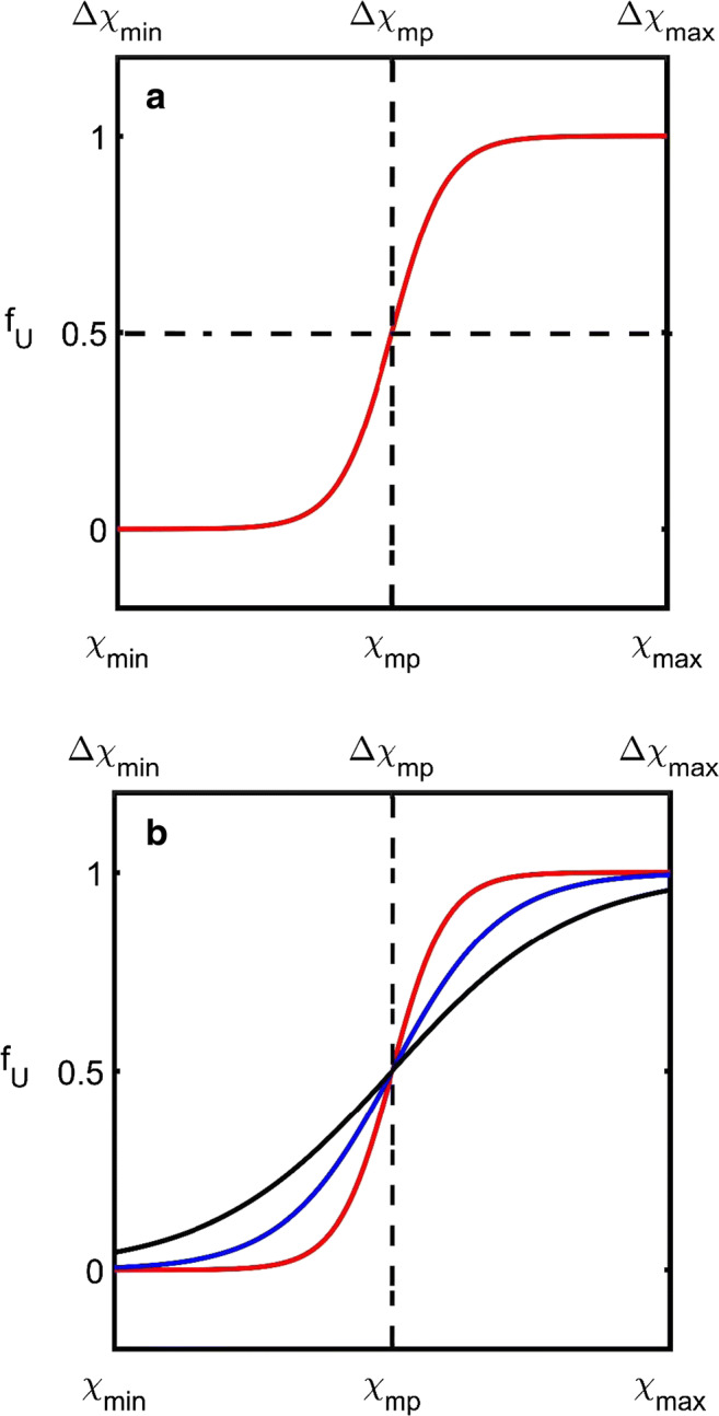
Midpoint characterization scheme. a Schematic showing the dependence of f_U, vs. χ (or Δχ) (i.e., fraction of unfolded protein upon the variable responsible for inducing change, e.g., temperature, pressure or denaturing solute, or miscible solvent). The domain of interest for analysis lies between lower (χ_min or Δχ_min) and upper bounds (χ_max or Δχ_max) which respectively define the operating range between f_U ≈ 0 and f_U ≈ 1. A single parameter χ_mp (or Δχ_mp) at which f_U is equal to 0.5 is used to characterize the data. b Deficiency of the midpoint characterization scheme: three different unfolding curves (red, blue, and black) are all characterized by the same value of χ_mp. With only one parameter, the midpoint characterization scheme cannot describe the steepness of the transition between folded and unfolded states. (Translated and reprinted with full permission from Wakayama et al. (2019))

Empirical scheme 1: midpoint analysis

Depending on experimental design, one may either measure the dependence of f_U on the absolute value of the independent variable, χ, or on its absolute difference, Δχ, between some reference value, χ₁ and the progressed value of that variable, χ₂ (Fig. 1a). Given that the means for affecting the protein-folded state typically involves altering system temperature, pressure, or composition, by far, the vast majority of published unfolding experiments are presented as either f_U vs. T (or ΔT), f_U vs. P (or ΔP) or f_U vs. C_D (or ΔC_D) (where C_D refers to the concentration of denaturant) (Eftink and Ionescu 1997; Fersht 1999). The simplest procedure for characterizing unfolding curves involves their reduction to a single parameter describing their transition midpoint (mp), i.e., the value of χ_mp at which f_U = 0.5 (Fig. 1a). Such an empirical analysis has the advantage that it is entirely general and can, in the ideal case, be used to rank solvents according to their capacity for protein stabilization (Fersht 1999; Pfeil 2012; Kumar et al. 2017). However, such a procedure provides no information on the transition path adopted and can therefore potentially miss important additional aspects of protein stability associated with the thermodynamic pathway (Fig. 1b). One such matter is enzyme loss due to aggregation (Roberts 2007; Weingartner et al. 2012; Kamal et al. 2016). Unfolded proteins exhibit a strong tendency to aggregate in a concentration-dependent manner to form either amorphous or structured aggregates (Chi et al. 2003; Mezzenga and Fischer 2013) (with amyloid fibers being one prominent example of a structured aggregate class having relevance to disease and biotechnology (Stefani and Dobson 2003; Hall 2003; Hall and Hirota 2009; Hall and Huang 2012; Hall 2012; Hall and Edskes 2004, 2009, 2012)). In any multi-parameter optimization procedure, conditions are modified to achieve the best system performance and therefore care must be taken that the adjustable factors such as temperature, pressure, solvent composition, and enzyme concentration do not adversely affect enzyme stability and activity (Rogers and Bommarius 2010; Lima-Ramos et al. 2014). As such, knowing how far below the unfolding midpoint to set reaction conditions that minimize loss of protein due to protein aggregation but do not miss out on the catalytic benefits of an altered value of χ is vital to efficient process design (Fields 2001; Bommarius 2015). The inability of the midpoint analysis to provide information on the steepness and breadth of the unfolding transition can be rectified using a slightly more complex two-parameter empirical characterization procedure known as the m-value approach (Greene and Pace 1974; Pace 1986), which will be discussed in the next section.

Empirical scheme 2: m value approach

In practice, an equilibrium constant reflecting the extent of protein unfolding can be determined for each set of conditions producing a different measured value of f_U (Fig. 2a). In a series of papers in the 1970s and 1980s Green and Pace (Greene and Pace 1974; Pace 1986; Pace and Shaw 2000) noted that the logarithm of the unfolding equilibrium constant frequently exhibited a linear dependence on Δχ. In cases of non-linearity, an additional term (or terms), extending to a polynomial dependence, sufficed to provide a description of the system (Myers et al. 1995; Johnson and Fersht 1995; Eftink and Ionescu 1997; Nicholson and Scholtz 1996; O’Brien et al. 2009; this work). Although we will approach this point later in a more formal fashion, for now, we express this concept generally by noting that the equilibrium constant, for any reversible process, can be expressed in terms of the standard state molar free energy change between reactants and products, Δg°_FU, along with any additional free energy change, d(Δg°_FU (Δχ)), undergone by that system as a consequence of the change Δχ (Eq. 2).

Fig. 2.

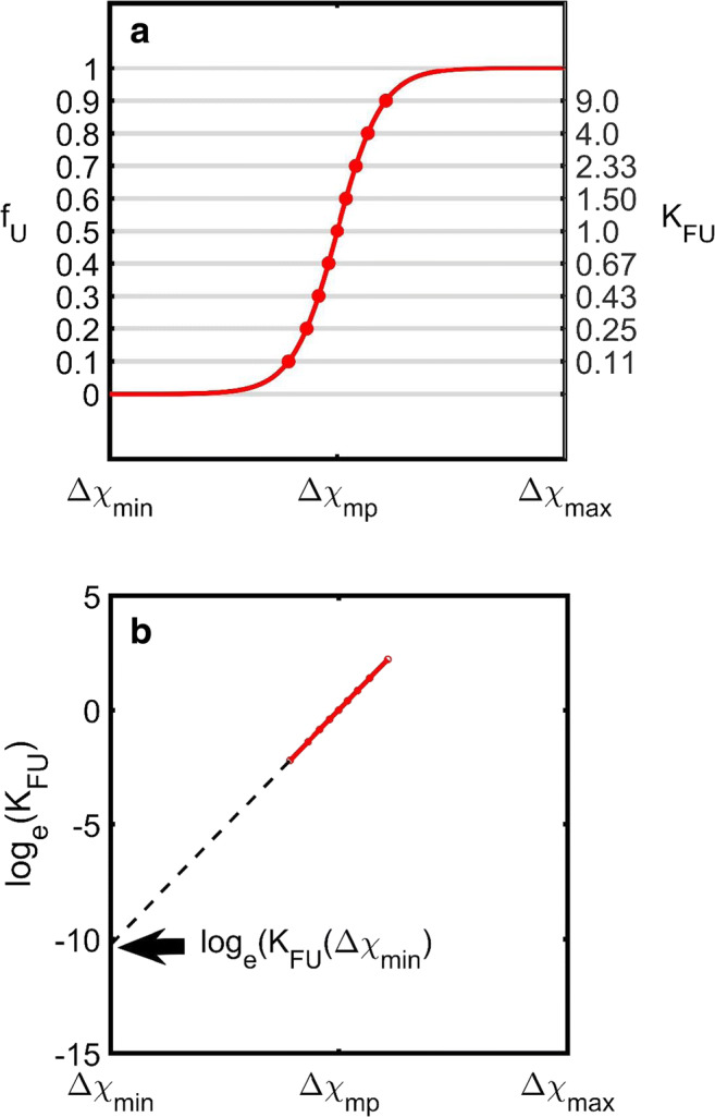
Generalized m value approach. a Simulated dependence of f_U, upon Δχ generated using the m value procedure (Eq. 5). This approach is able to account for the shape of the transition pathway based on just two parameters, the unfolding midpoint, χ_mp, and the m value (defined as $m={\left[\frac{d\left(∆g_{\mathit{FU}}^{°}\right)}{d\mathrm{\Delta }\chi }\right]}_{\mathrm{\Delta }\chi =0}$). b Historically speaking, the m value approach was based on experimental observations of a linear dependence of log_e(K_FU) upon the variable χ inducing the change. In this approach, values of K_FU were first evaluated from f_U (via Eq. 1c) at each point on the f_U vs. Δχ unfolding curve. Typically, noise within the data set only allowed points significantly removed from the extrema to be used in the estimation of K_FU, i.e., 0.1 < f_U < 0.9. From a plot log_e(K_FU) against Δχ a value of log_e(K_FU) at some reference state χ_min could be determined by linear extrapolation. (Translated and reprinted with full permission from Wakayama et al. (2019))

$${\left(K_{\mathit{FU}}\right)}_{∆\chi }=exp\left(\frac{-\left[∆g{°}_{\mathit{FU}}+d\left(∆g{°}_{\mathit{FU}}\left(\mathrm{\Delta \chi }\right)\right)\right]}{\mathit{RT}}\right)$$ 2a

$${log}_e{\left(K_{\mathit{FU}}\right)}_{∆\chi }={log}_e{\left(K_{\mathit{FU}}\right)}_{∆\chi =0}-\left(\frac{1}{\mathit{RT}}\right)\left[d\left(∆g{°}_{\mathit{FU}}\left(\mathrm{\Delta \chi }\right)\right)\right]$$ 2b

The additional free energy term d(∆g°_FU) can be described as a function of Δχ using a Taylor expansion about the point (Δχ = 0, ∆g°_FU) (Eq. 3a). The often noted apparent linear dependence of a plot of log_e(K_FU)_Δχ upon Δχ (Auton and Bolen 2005; Myers et al. 1995; O’Brien et al. 2009) can be seen as a case of the adequacy of truncation of the Taylor expansion at the first term. This first derivative term was named as the m value by Pace and co-workers (Eq. 3b; Greene and Pace 1974).

$$d∆g{°}_{\mathit{FU}}\left(\mathrm{\Delta \chi }\right)={\left(\frac{d\left(∆g_{\mathit{FU}}^{°}\right)}{d\mathrm{\Delta }\chi }\right)}_{\mathrm{\Delta }\chi =0}.\mathrm{\Delta \chi }+\frac{1}{2}{\left(\frac{d^2\left(∆g_{\mathit{FU}}^{°}\right)}{{d\mathrm{\Delta }\chi }^2}\right)}_{\mathrm{\Delta }\chi =0}.{\left(\mathrm{\Delta \chi }\right)}^2+...$$ 3a

$$m_{\chi }={\left(\frac{d\left(∆g_{\mathit{FU}}^{°}\right)}{d\mathrm{\Delta }\chi }\right)}_{\mathrm{\Delta }\chi =0}$$ 3b

For mathematical utility, the standard-state free energy is typically defined with regard to the midpoint of the unfolding transition (χ_mp)—a point at which Δχ = 0, C_U = C_F, (K_FU)_Δχ = 0 = 1, and Δg°_FU (Δχ = 0) = 0. Depending on the nature of the change (i.e., Δχ = ΔP, ΔT, or Δn_D (or as more commonly used ΔC_D)), the terms in the free energy derivative with respect to the change will differ. Here, we take a liberty in order to simplify the literature somewhat by employing the m value terminology coined originally for denaturant-induced unfolding (Greene and Pace 1974) for each of the three main methods for inducing protein unfolding, such that we have an m value for temperature, m_T (Eq. 4a), for pressure, m_P (Eq. 4b), and for denaturant, m_D (Eq. 4c).

$$m_T={\left(\frac{d\left(∆g_{\mathit{FU}}^{°}\right)}{d\mathrm{\Delta }T}\right)}_{\mathrm{\Delta }T=0}$$ 4a

$$m_P={\left(\frac{d\left(∆g_{\mathit{FU}}^{°}\right)}{d\mathrm{\Delta }P}\right)}_{\mathrm{\Delta }P=0}$$ 4b

$$m_D={\left(\frac{d\left(∆g_{\mathit{FU}}^{°}\right)}{d{\mathrm{\Delta }C}_D}\right)}_{\mathrm{\Delta }{C}_D=0}$$ 4c

Using this approach, protein unfolding curves may be minimally characterized using two parameters, the characteristic “m value” and the transition midpoint χ_mp. Inserting the necessary terms for the description of K_FU at different values of χ into Eq. 1c yields Eq. 5 which can be used in non-linear regression analysis of f_U vs. χ data to provide estimates of the two relevant parameters χ_mp and m_χ.

$$f_U=\frac{exp\left(\frac{-m_{\chi }.\left(\chi -{\chi }_{\mathit{mp}}\right)}{R.T}\right)}{1+exp\left(\frac{-m_{\chi }.\left(\chi -{\chi }_{\mathit{mp}}\right)}{R.T}\right)}$$ 5

An important consequence of the m value procedure is that the difference in free energy between some additional reference state and the transition midpoint can be obtained via linear extrapolation allowing the intrinsic (unperturbed) stability of the protein to be estimated (Fig. 2b). For this reason, the m value procedure is sometimes called the linear extrapolation method (LEM) (Tanford 1970; Greene and Pace 1974; Pace 1986; Santoro and Bolen 1988; Auton and Bolen 2005). Despite the simplicity and obvious usefulness of the m value/LEM procedure, due to its empirical nature, it lacks mechanistic insight into the molecular causes of the unfolding reaction. In the following sections, we present some theory-based characterization procedures that rectify this problem.

Mechanistic approaches for characterizing protein folding based on classical thermodynamics

Noting the demonstrated success of the m value/LEM procedure described in the previous section, it will be instructive to examine the theoretical reasons as to (i) why such a linear extrapolation method is often observed to hold true in practice and (ii) what situations would lead to its invalidity. For the sake of making this section easily digestible, a general discussion of the thermodynamics of open systems containing components able to partake in reversible chemical equilibrium is provided as Appendix 1. Based on the material introduced therein, we develop our subsequent argument from a starting point provided by the three equations presented as Eq. 6. Briefly, Eq. 6a is concerned with the use of the chemical potential of the folded, μ_F, and unfolded, μ_U, protein species to define the condition for chemical equilibrium, Eq. 6b describes the method for incorporating change into the chemical potential upon a change in the reaction conditions [T₁, P₁, {n_j}₁ → T₂, P₂, {n_j}₂] and Eq. 6c describes the procedure for calculating the extent of change in chemical potential upon a change in conditions.4

$${\left({\mathrm{\mu }}_U\right)}_{T_2,P_2,{\left\{n_j\right\}}_2}={\left({\mathrm{\mu }}_F\right)}_{T_2,P_2,{\left\{n_j\right\}}_2}$$ 6a

$${\left({\mathrm{\mu }}_i\right)}_{T_2,P_2,{\left\{n_j\right\}}_2}={\left({\mathrm{\mu }}_i\right)}_{T_1,P_1,{\left\{n_j\right\}}_1}+{\left(d{\mu }_i\right)}_{T_1,P_1,{\left\{n_j\right\}}_1\to T_2,P_2,{\left\{n_j\right\}}_2}$$ 6b

$${\left(d{\mu }_i\right)}_{T_1,P_1,{\left\{n_j\right\}}_1\to T_2,P_2,{\left\{n_j\right\}}_2}={\left(\partial {\mu }_i\right)}_{T_1\to T_2;P,\left\{n_j\right\}}+{\left(\partial {\mu }_i\right)}_{P_1\to P_2;T,\left\{n_j\right\}}+{\sum }_{j=1}^Q{\left(\frac{\partial {\mu }_j}{\partial n_i}\right)}_{{\left(n_i\right)}_1\to {\left(n_i\right)}_2;T,P,\left\{n_{i\ne k}\right\}}.d{n}_j$$ 6c

On the back of these three equations, we derive analytical relations that describe the effect of change in temperature, pressure or concentration of added denaturant upon the unfolding equilibrium constant.

Temperature-induced unfolding

A thermally induced change in the concentration of the ith component, occurring at constant pressure and concentration of other solution components, implies that the equation describing the change in chemical potential will only include two of the Q + 2 possible transitions from Eq. 6c, ${\left(\partial {\mu }_i\right)}_{T_1\to T_2;P,\left\{n_j\right\}}$ and ${\left(\partial {\mu }_i\right)}_{{\left(n_i\right)}_1\to {\left(n_i\right)}_2,T,P,\left\{n_{j\ne i}\right\}}$ (Eq. 7a). The chemical potential of the folded and unfolded protein forms at a new set of conditions (calculated according to Eq. 6b) can be respectively described by equations shown as Eq. 7b and c. For clarity, we have used curly brackets to contain the terms constituting the species chemical potential at the initial condition set (T₁, P₁, {n_j}₁) and the ∂μ terms just for the temperature (T₁ → T₂) and concentration ((n_i)₁ → (n_i)₂) transitions (as described in Eq. 6c). Small letters are used to denote the partial molar change in a quantity such that s_i and h_i respectively represent the partial molar change in system entropy and enthalpy for component i (i.e., s_i = ${\left(\frac{\mathrm{\partial S}}{\partial n_i}\right)}_{T,P,\left\{n_{j\ne i}\right\}}$ and h_i = ${\left(\frac{\mathrm{\partial H}}{\partial n_i}\right)}_{T,P,\left\{n_{j\ne i}\right\}}$)

$${\left(d{\mu }_i\right)}_{T_1\to T_2,{\left(n_i\right)}_1\to {\left(n_i\right)}_2;P,\left\{n_{j\ne i}\right\}}={\left(\partial {\mu }_i\right)}_{T_1\to T_2;P,\left\{n_j\right\}}+{\left(\partial {\mu }_i\right)}_{{\left(n_i\right)}_1\to {\left(n_i\right)}_2;T,P,\left\{n_{j\ne i}\right\}}$$ 7a

$${\left({\mu }_F\right)}_{T_{2}P,{\left\{n_{j\ne F}\right\}}_2}=\left\{{\left({\mu }_F^{°}\right)}_{T_1,P,{\left\{n_{j\ne F}\right\}}_1}+R{T}_1\mathit{lo}{g}_e\left(\frac{{\left(C_F\right)}_1}{C_F^{°}}\right)\right\}+\left\{-{\int }_{T_1}^{T_2}{s}_F.\mathit{dT}\right\}+\left\{R{T}_1{\mathit{log}}_e\left(\frac{{\left(C_F\right)}_2}{{\left(C_F\right)}_1}\right)\right\}$$ 7b

$${\left({\mu }_U\right)}_{T_2,P,{\left\{n_{j\ne U}\right\}}_2}=\left\{{\left({\mu }_U^{°}\right)}_{T_1,P,{\left\{n_{j\ne U}\right\}}_1}+R{T}_1\mathit{lo}{g}_e\left(\frac{{\left(C_U\right)}_1}{C_U^{°}}\right)\right\}+\left\{-{\int }_{T_1}^{T_2}{s}_U.\mathit{dT}\right\}+\left\{R{T}_1{\mathit{log}}_e\left(\frac{{\left(C_U\right)}_2}{{\left(C_U\right)}_1}\right)\right\}$$ 7c

Inserting these relations into the condition for a two-state equilibrium between folded and unfolded states (Eq. 6a) yields Eq. 8.

$$-R{log}_e\left(\frac{C_{U\left\{2\right\}}.C_F^{°}}{C_{F\left\{2\right\}}.C_U^{°}}\right)=\left(\frac{1}{T_1}\right).\left(\Delta {\mu }_{\mathit{FU}}^{°}-{\int }_{T_1}^{T_2}\Delta s_{\mathit{FU}}.\mathit{dT}\right)$$ 8a

$$∆{\mu }_{\mathit{FU}}^{°}={\left({\mu }_U^{°}\right)}_{T_1,P_1,{\left\{n_{j\ne U}\right\}}_1}-{\left({\mu }_F^{°}\right)}_{T_1,P_1,{\left\{n_{j\ne F}\right\}}_1}$$ 8b

$$\Delta s_{\mathit{FU}}=\left(s_U-s_F\right)$$ 8c

In order to calculate the change in entropy of the system at a fixed temperature with regard to change in the number of moles of either the folded or unfolded species, we note that the standard state chemical potential of component i appearing in Eq. A2c, μ_i^°, can be expressed in terms of its component standard state enthalpy, h_i^°, and entropy, s_i^°, with this substitution allowing construction of Eq. 9.

$$∆{\mu }_{\mathit{FU}}^{°}=\left(h_U^{°}-h_F^{°}\right)-T.\left(s_U^{°}-s_F^{°}\right)$$ 9

If a set of conditions [T₁, P₁, {n_j}₁] is selected such that $∆{\mu }_{\mathit{FU}}^{°}$ = 0, Eq. 9 can be rearranged to Eq. 10.

$$∆s_{\mathit{FU}}^{°}=\frac{∆h_{\mathit{FU}}^{°}}{T_1}$$ 10

We may calculate the value of Δs_FU at a different temperature by introducing the concept of heat capacity (Shiao et al. 1971; Privalov and Khechinashvili 1974; Sturtevant 1977; Becktel and Schellman 1987; Van Holde et al. 2006a). For small changes in temperature, the molar system enthalpy at a temperature T₂ can be determined from its value at a reference temperature, T₁, using a linear approximation (Eq. 11a). Equation 11a can be further differentiated with respect to changes in composition allowing the partial molar enthalpy of unfolding, ∆h_FU , at a second temperature to be determined using Eq. 11b.

$$H_{\text{system}}\left(T_2\right)=H_{\text{system}}^{°}\left(T_1\right)+\mathrm{\Psi }.\mathit{dT}$$ 11a

$${\left(\Delta h_{\mathit{FU}}\right)}_{T_2,P_1,{\left\{n_j\right\}}_2}={\left(\Delta h_{\mathit{FU}}^{°}\right)}_{T_1,P_1,{\left\{n_j\right\}}_2}+{\int }_{T_1}^{T_2}{\left(\Delta {\sigma }_{\mathit{FU}}\right)}_{P_1,{\left\{n_j\right\}}_2}.\mathit{dT}$$ 11b

Here, Ψ describes the heat capacity at constant pressure, i.e., the differential change in system enthalpy with change in temperature, i.e., $\psi ={\left(\frac{\partial H^{°}}{\partial T}\right)}_{P,\left\{n_j\right\}}$ and Δσ_FU describes the difference in the partial derivatives of Ψ with regard to U and F species such that, ${\left({∆\sigma }_{\mathit{FU}}\right)}_{P,\left\{n_j\right\}}={\left(\frac{\mathrm{\partial \Psi }}{\partial n_U}\right)}_{P,\left\{n_{j\ne U}\right\}}-{\left(\frac{\mathrm{\partial \Psi }}{\partial n_F}\right)}_{P,\left\{n_{j\ne F}\right\}}$. Using the formalism shown in Eqs. 10 and 11, the partial molar change in system entropy for the unfolding reaction at a different temperature, Δs_FU(T), can be estimated by expanding around the exact result defined at T₁ in Eq. 12.5

$$\Delta s_{\mathit{FU}}\left(T_1\right)=\left(\frac{\Delta h_{\mathit{FU}}^{°}+\Delta {\sigma }_{\mathit{FU}}.\mathit{\Delta T}}{T_1}\right)$$ 12

Inserting Eq. 12 into Eq. 8a followed by integration and then multiplication through by T₂ yields Eq. 13a. Subsequent rearrangement and taking the anti-logarithm produces Eq. 13b.

$$-R{T}_2{log}_e\left(\frac{C_{U\left\{2\right\}}.C_F^{°}}{C_{F\left\{2\right\}}.C_U^{°}}\right)=\left(\frac{T_2}{T_1}\right).{\left(\mathrm{\Delta }{\mu }_{\mathit{FU}}^{°}\right)}_{T_1,P_1,{\left\{n_j\right\}}_1}+\left[{\mathrm{\Delta }h}_{\mathit{FU}}^{°}.\left(1-\frac{T_2.}{T_1}\right)-{\mathrm{\Delta }\sigma }_{\mathit{FU}}.\left(T_2.\mathrm{lo}{\mathrm{g}}_e\left(\frac{T_2}{T_1}\right)-\left(T_2-T_1\right)\right)\right]$$ 13a

$${\left(K_{\mathit{FU}}\right)}_{T_2,P_1,{\left\{n_j\right\}}_2}=\left[{\left(K_{\mathit{FU}}\right)}_{T_1,P_1,{\left\{n_j\right\}}_1}\right].exp\left\{\frac{-\left[{\mathrm{\Delta }h}_{\mathit{FU}}^{°}.\left(1-\frac{T_2.}{T_1}\right)+\mathrm{\Delta }{\sigma }_{\mathit{FU}}.\left(T_2-T_1\right)-{\mathrm{\Delta }\sigma }_{\mathit{FU}}.T_2.\mathrm{lo}{\mathrm{g}}_e\left(\frac{T_2}{T_1}\right)\right]}{R{T}_2}\right\}$$ 13b

One interesting aspect of Eq. 13 is associated with the definition of T₁. This temperature must be set as the midpoint of the unfolding transition, i.e., T₁ = T_mp, to satisfy the standard state requirement in Eq. 10a and thus, by definition${\left(\mathrm{\Delta }{\mu }_{\mathit{FU}}^{°}\right)}_{T_1,P_1,{\left\{n_j\right\}}_1}=0$; C_F = C_U, and ${\left(K_{\mathit{FU}}\right)}_{T_1,P_1,{\left\{n_j\right\}}_1}=1$. Inserting this description of K_FU into Eq. 1c provides a three parameter (T_mp, Δh^°_FU, and Δσ_FU) expression (Eq. 14) useful for non-linear regression analysis of f_U vs. T data (Fig. 3a).

$$f_U=\frac{exp\left\{\frac{-\left[{\mathrm{\Delta }h}_{\mathit{FU}}^{°}.\left(1-\frac{T_2.}{T_{\mathit{mp}}}\right)+\mathrm{\Delta }{\sigma }_{\mathit{FU}}.\left(T_2-T_{\mathit{mp}}\right)-{\mathrm{\Delta }\sigma }_{\mathit{FU}}.T_2.\mathrm{lo}{\mathrm{g}}_e\left(\frac{T_2}{T_{\mathit{mp}}}\right)\right]}{R{T}_2}\right\}}{1+exp\left\{\frac{-\left[{\mathrm{\Delta }h}_{\mathit{FU}}^{°}.\left(1-\frac{T_2.}{T_{\mathit{mp}}}\right)+\mathrm{\Delta }{\sigma }_{\mathit{FU}}.\left(T_2-T_{\mathit{mp}}\right)-{\mathrm{\Delta }\sigma }_{\mathrm{F}U}.T_2.\mathrm{lo}{\mathrm{g}}_e\left(\frac{T_2}{T_{\mathit{mp}}}\right)\right]}{R{T}_2}\right\}}$$ 14

Fig. 3.

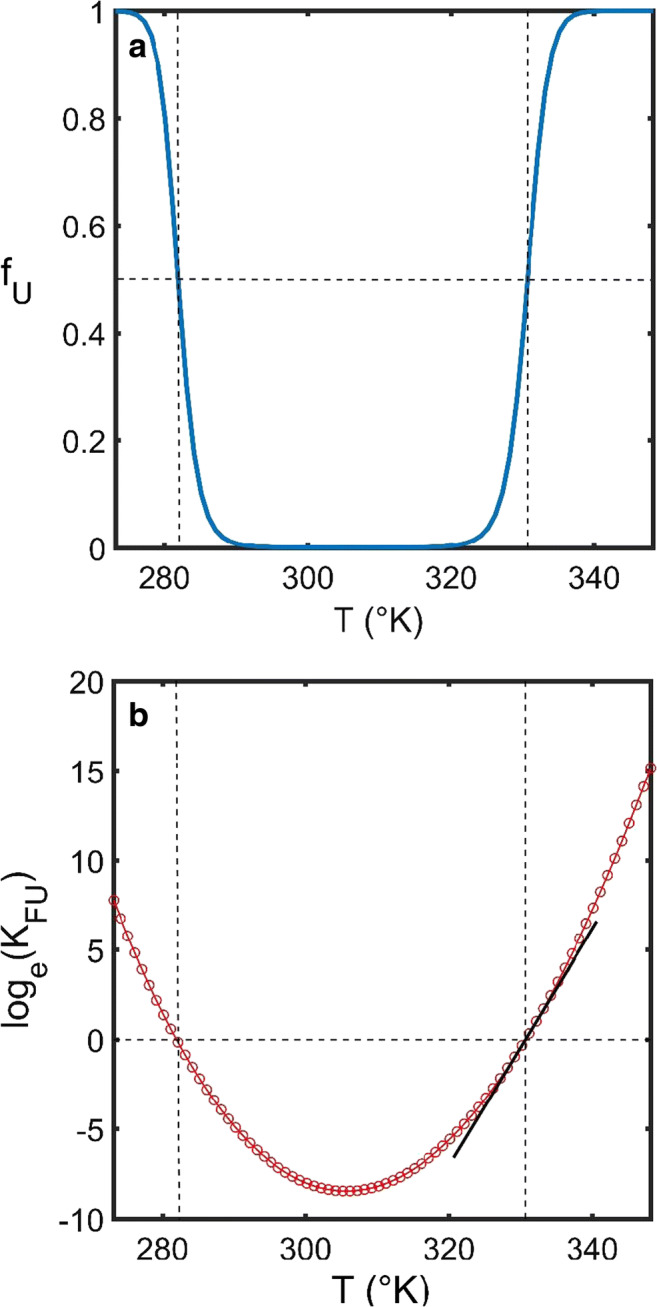
Temperature-induced unfolding. a Simulated dependence of the fraction of unfolded protein upon temperature (f_U upon T) generated using the Gibbs-Helmholtz equation (Eq. 12). As formulated, the Gibbs-Helmholtz expression is based on three independent parameters, the heat-induced unfolding mid-point, T_mp, the change in molar enthalpy upon unfolding, Δh_FU, and the change in molar heat capacity upon unfolding, Δσ_FU. Note that the appearance of the cold induced unfolded region at low temperatures. b A plot of log(K_FU) vs. T is typically not linear due to the additional molar heat capacity term (Δσ_FU) which accounts for changes in the enthalpy of unfolding at different temperatures. As such, the m_T value predicted in Eq. 4a will only describe the slope at the heat-induced transition midpoint, T_mp. [Parameter values used in the simulation were Δh_FU = 6 × 10⁵ J mol⁻¹, Δσ_FU = 2.4 × 10⁴ J K⁻¹ mol⁻¹ and T_mp = 57.5 °C]. (Translated and reprinted with full permission from Wakayama et al. (2019))

In terms of explaining the dependence (linear or otherwise) of log_e(K_FU) upon ΔT, we note that Eq. 13b can be rearranged to Eq. 15a—a further simplification of which can be made (Eq. 15b) by noting6 that for small deviations from the midpoint log_e(T₂/T_mp) ≈ (T₂−T_mp)/T_mp (Fig. 3b).

$${log}_e\left[{\left(K_{\mathit{FU}}\right)}_{T_2,P_1,{\left\{n_j\right\}}_2}\right]=\left(\frac{1}{R{T}_2}\right)\left\{-\left[{\mathrm{\Delta }h}_{\mathit{FU}}^{°}.\left(\frac{T_2-T_{\mathit{mp}}}{T_{\mathit{mp}}}\right)+\mathrm{\Delta }{\sigma }_{\mathit{FU}}.\left(T_2-T_{\mathit{mp}}\right)-{\mathrm{\Delta }\sigma }_{\mathit{FU}}.T_2.\mathrm{lo}{\mathrm{g}}_e\left(\frac{T_2}{T_{\mathit{mp}}}\right)\right]\right\}$$ 15a

$${log}_e\left[{\left(K_{\mathit{FU}}\right)}_{T_2,P_1,{\left\{n_j\right\}}_2}\right]\approx \frac{-\mathrm{\Delta }{h}_{\mathit{FU}}^{°}}{R.{T_{\mathit{mp}}}^2}.∆T$$ 15b

The above two equations (Eq. 15a and b) are sufficient to understand why and under what regimes an m value-type description can represent a good approximation for thermal unfolding, i.e., Eq. 15b will hold for small changes in temperature but curvature should become apparent for larger temperature deviations or alternatively, when the system heat capacity is so sensitive to temperature change that it may not be described using a linear approximation. Importantly, Eq. 15 allows for the mechanistic interpretation of a ${log}_e\left[{\left(K_{\mathit{FU}}\right)}_{T_2,P_1,{\left\{n_j\right\}}_2}\right]$ vs. T-type plot. Around the midpoint, the slope7 will be equal to − Δh_FU/(RT_mp²) (Fig. 3b) and the m_T value (as defined by Eq. 4a) will be approximately equal to − Δh_FU/T_mp). At positions farther away from the midpoint, the general slope of the ${log}_e\left[{\left(K_{\mathit{FU}}\right)}_{T_2,P_1,{\left\{n_j\right\}}_2}\right]$ vs. ΔT plot will be a complex non-constant function given by $\left(\frac{-1}{R{T}_2}\right)\left[{\mathrm{\Delta }h}_{\mathit{FU}}^{°}/T_{\mathit{mp}}+\mathrm{\Delta }{\sigma }_{\mathit{FU}}-\frac{\left[{\mathrm{\Delta }\sigma }_{\mathit{FU}}.T_2.\mathrm{lo}{\mathrm{g}}_e\left(\frac{T_2}{T_{\mathit{mp}}}\right)\right]}{\left(T_2-T_{\mathit{mp}}\right)}\right]$. Interestingly, the non-constant slope term contained within Eq. 15a provides the necessary thermodynamic formulation to quantitatively “understand” the phenomenon of low-temperature-induced protein unfolding—sometimes termed cold denaturation (Privalov 2007; Fig. 3). With a greater possible range of temperatures for the liquid state, such considerations will be important when interpreting the behavior of protein folding in ionic liquid media (Constantinescu et al. 2007; Constatinescu et al. 2010; Satish et al. 2016; Brogan and Hallett 2016).

Pressure-induced unfolding

The volume, V, of a multicomponent system can be expressed in terms of the sum of the number of moles of each component multiplied by their partial molar volume, ${\left({\mathrm{\upsilon }}_i\right)}_{T,P,\left\{n_j\right\}}$, where ${\left({\mathrm{\upsilon }}_i\right)}_{T,P,\left\{n_j\right\}}={\left(\frac{\mathrm{\partial V}}{\partial n_i}\right)}_{T,P,\left\{n_j\right\}}$(Eq. 16). Assuming that the partial molar volume does not depend upon type and concentration of other components (Van Holde et al. 2006b) allows Eq. 16a to be approximated by Eq. 16b.

$${\left(\mathrm{V}\right)}_{T,P,\left\{n_j\right\}}={\sum }_{i=1}^Q{\int }_0^{n_i}{\left(\frac{\mathrm{\partial V}}{\partial n_i}\right)}_{T,P,\left\{n_j\right\}}.d{n}_i$$ 16a

$${\left(\mathrm{V}\right)}_{T,P,\left\{n_j\right\}}\approx {\sum }_{i=1}^Q{n}_i.{\left({\mathrm{\upsilon }}_i\right)}_{T,P}$$ 16b

At constant temperature but altered pressure, the chemical potentials for folded and unfolded protein forms at a new set of conditions (T₁, P₂,{n_j}₂) corresponding to changes in P and {n_j} are respectively given by Eq. 6b and c (resulting in Eq. 17a and b). Again, curly brackets are used to indicate terms arising from change in chemical potential, dμ, (via Eq. 6c).

$${\left({\mu }_F\right)}_{T_1,P_2,{\left\{n_j\right\}}_2}=\left\{{\left({\mu }_F^{°}\right)}_{T_1,P_1,{\left\{n_{j\ne F}\right\}}_1}+R{T}_1\mathit{ln}\left(\frac{{\left(C_F\right)}_1}{C_F^{°}}\right)\right\}+\left\{{\int }_{P_1}^{P_2}{\left(\frac{\mathrm{\partial V}}{\partial n_F}\right)}_{T_1,P,{\left\{n_{j\ne F}\right\}}_2}.\mathit{dP}\right\}+\left\{R{T}_1\mathit{ln}\left(\frac{{\left(C_F\right)}_2}{{\left(C_F\right)}_1}\right)\right\}$$ 17a

$${\left({\mu }_U\right)}_{T_1,P_2,{\left\{n_j\right\}}_2}=\left\{{\left({\mu }_U^{°}\right)}_{T_1,P_1,{\left\{n_{j\ne U}\right\}}_1}+R{T}_1\mathit{ln}\left(\frac{{\left(C_U\right)}_1}{C_U^{°}}\right)\right\}+\left\{{\int }_{P_1}^{P_2}{\left(\frac{\mathrm{\partial V}}{\partial n_U}\right)}_{T_1,P,{\left\{n_{j\ne U}\right\}}_2}.\mathit{dP}\right\}+\left\{R{T}_1\mathit{ln}\left(\frac{{\left(C_U\right)}_2}{{\left(C_U\right)}_1}\right)\right\}$$ 17b

With the additional assumption that the partial molar volume for both folded, υ_F, and unfolded forms, υ_U, of protein are independent of pressure, the above expressions can be further simplified and inserted into the equilibrium relation shown by Eq. 6a to produce Eq. 18a which, with subsequent rearrangement, produces Eq. 18b.

$${\left({\mu }_F^{°}\right)}_{T_1,P_1,{\left\{n_j\right\}}_1}+{\int }_{P_1}^{P_2}{\upsilon }_F.\mathit{dP}+R{T}_1\mathit{ln}\left(\frac{{\left(C_F\right)}_2}{C_F^{°}}\right)\approx {\left({\mu }_U^{°}\right)}_{T_1,P_1,{\left\{n_j\right\}}_1}+{\int }_{P_1}^{P_2}{\upsilon }_U.\mathit{dP}+R{T}_1\mathit{ln}\left(\frac{{\left(C_U\right)}_2}{C_U^{°}}\right)$$ 18a

$$-R{T}_1\mathit{ln}\left(\frac{{\left(C_U\right)}_2.C_F^{\circ }}{{\left(C_F\right)}_2.C_U^{\circ }}\right)={\left({\mu }_U^{°}\right)}_{T_1,P_1,{\left\{n_{j\ne U}\right\}}_1}-{\left({\mu }_F^{°}\right)}_{T_1,P_1,{\left\{n_{j\ne F}\right\}}_1}+{\int }_{P_1}^{P_2}\left({\upsilon }_U-{\upsilon }_F\right).\mathit{dP}$$ 18b

Integration of Eq. 18b yields a result for the equilibrium constant (Eq. 19a) which may be further simplified (Eq. 19b) (which is the analytical form most often used in the treatment of data; Mozhaev et al. 1996; Fersht 1999; Sasahara et al. 2001; Pandharipande and Makhatadze 2016).

$${\left({\mathrm{K}}_{\mathit{FU}}\right)}_{T_1,P_2,{\left\{n_j\right\}}_2}=\left(\frac{{\left(C_U\right)}_2.C_F^{\circ }}{{\left(C_F\right)}_2.C_U^{\circ }}\right)=exp\left(\frac{-\left[{\left({\mu }_U^{°}\right)}_{T_1,P_1,{\left\{n_{j\ne U}\right\}}_1}-{\left({\mu }_F^{°}\right)}_{T_1,P_1,{\left\{n_{j\ne F}\right\}}_1}\right]-\Delta {\upsilon }_{\mathit{FU}}.\left[P_2-P_1\right]}{R{T}_1}\right)$$ 19a

$${\left(K_{\mathit{FU}}\right)}_{T_1,P_2,{\left\{n_j\right\}}_2}=\left[{\left(K_{\mathit{FU}}\right)}_{T_1,P_1,{\left\{n_j\right\}}_1}\right].exp\left[\frac{-\Delta {\upsilon }_{\mathit{FU}}.\left[P_2-P_1\right]}{R{T}_1}\right]$$ 19b

If the initial state pressure, P₁, is chosen as the midpoint of the unfolding transition, P_mp, then by definition, the equilibrium constant at this pressure is equal to 1, i.e., ${\left(K_{\mathit{FU}}\right)}_{T_1,P_1,{\left\{n_j\right\}}_1}=1$ and C_F = C_U (Fig. 4a). Inserting this expression for K_FU into Eq. 1c provides an equation consisting of two parameters (P_mp and Δυ_FU) that can be used directly in non-linear regression analysis of f_U vs. P unfolding data (Eq. 20a; Fig. 4a). Interestingly, as a non-colligative parameter, the change in partial molar volume, Δυ_FU, will be dependent upon the molecular mass of the protein M_P (units kg/mol) and the change in partial specific volume upon unfolding, Δv_FU, with this latter quantity defined in terms of volume per weight concentration (units m³/kg) such that Δυ_FU = M_PΔv_FU. This feature introduces an underappreciated protein size dependence to the pressure-induced unfolding experiment (Fig. 4b).

Fig. 4.

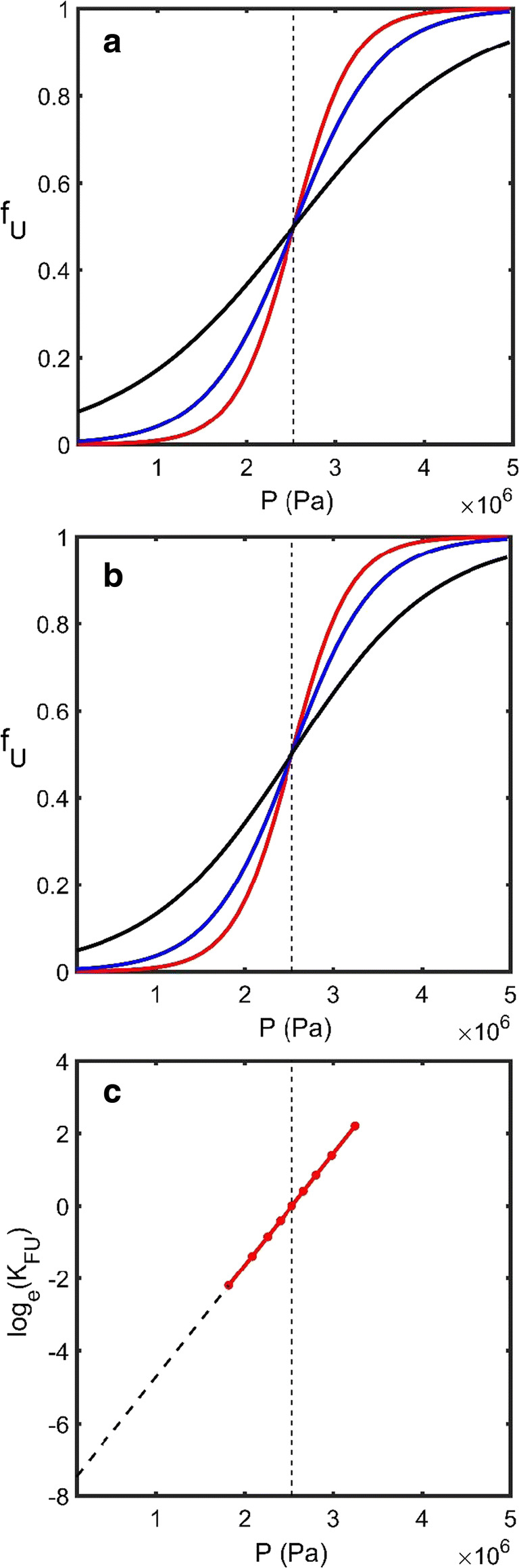
Pressure-induced unfolding. a Simulated dependence of the fraction of unfolded protein upon pressure (f_U upon P) generated using Eq.18 which is based upon two parameters, the molar volume change upon unfolding, Δυ_FU, and the pressure midpoint of the unfolding transition, P_mp. The pressure domain starts at standard atmospheric pressure, 101.3 kPa, and increases to 5 MPa. The red, blue, and black lines correspond to the pressure-induced unfolding transitions of three different proteins all jointly characterized by a mass M_p = 50,000 g/mol but respectively exhibiting three different values for Δυ_FU of − 0.15, 0.1 and 0.05 ml/g. b Simulated f_U upon P curves where red, blue, and black lines respectively describe the unfolding transitions of proteins possessing three different molecular masses M_p = 50,000, 35,000, and 20,000 g/mol but all exhibiting a common value for Δυ_FU of − 0.15 ml/g. c A plot of log(K_FU) vs. P will be linear if the assumptions made in the derivation of Eq. 18 hold. (Additional simulation parameters P_mp = 2.53 MPa, T = 20 °C]. (Translated and reprinted with full permission from Wakayama et al. (2019))

$$f_U=\frac{exp\left[\frac{-{∆\upsilon }_{\mathit{FU}}.\left[P_2-P_{\mathit{mp}}\right]}{R{T}_1}\right]}{1+exp\left[\frac{-{∆\upsilon }_{\mathit{FU}}.\left[P_2-P_{\mathit{mp}}\right]}{R{T}_1}\right]}$$ 20

Taking the logarithm of Eq. 19b yields Eq. 21.8

$${log}_e\left[{\left(K_{\mathit{FU}}\right)}_{T_1,P_2,{\left\{n_j\right\}}_2}\right]=\frac{-\Delta {\upsilon }_{\mathit{FU}}}{R{T}_1}.\left[P_2-P_1\right]$$ 21

Equation 21 is sufficient to achieve an understanding as to why the linear dependence prescribed by the m value/LEM approach represents a good approximation for pressure-induced unfolding (Fig. 4c). Equation 21 also allows for mechanistic interpretation of the meaning of the slope around the midpoint of a plot of log_e(${\left(K_{\mathit{FU}}\right)}_{T_1,P_2,{\left\{n_j\right\}}_2}$) vs. P, i.e., the slope will be equal to Δυ_FU/(RT₁) and the m_P value (as defined by Eq. 4b) will be equal to Δυ_FU. Furthermore, from the explicit listing of the two approximations in its derivation (Eq. 16b—υ_i is independent of composition and Eq. 18—υ_i is independent of the applied pressure), we can understand which assumptions are being violated when the m value/LEM is seen to not to be applicable (Eftink and Ionescu 1997; Fersht 1998; Pandharipande and Makhatadze 2016). Although not treated here, potential solvent compressibility issues associated with the diverse range of ionic liquids and their blends, represent an open question in this field (Seddon et al. 2000; Jacquemin et al. 2007).

Denaturant-induced unfolding

At constant temperature and pressure, a protein can be induced to unfold by replacement of the solvent components with chemicals which differentially stabilize the unfolded vs. folded state(s) (Anfinsen 1973). Such denaturant-induced unfolding may involve either specific or non-specific interaction between the added denaturants and the protein (whereby the assignment of the designation specific or non-specific is made on the basis of an affinity for the denaturant at a particular chemical site on the protein (Pace 1986; Schellman 2002; Hall et al. 2018)). This basic difference in consideration of specific vs. non-specific binding of denaturant is the underlying cause of the conceptual schism that has led to different theoretical formulations of the denaturant induced unfolding process (e.g., Schellman 1956; Aune and Tanford 1969 vs. Schellman 2002; Smiatek 2017 vs. Tanford 1968; O’Brien et al. 2009). Although each of these different approaches are logically consistent (and, importantly, mutually compatible [see Pace 1986 for an easy introduction]) due to its ease of construction, in what follows, we adopt the quantitative formulation for the specific binding format (Schellman 1958; Aune and Tanford 1969; Hall et al. 2018). We will consider three different states of the system that exist at an identical fixed temperature, T₁, and pressure, P₁, but differ with respect to the concentration of denaturant and reversible components. These three states defined as follows—state 0 [T₁, P₁,{n_j}₀, (C_D = 0)], state 1 [T₁, P₁,{n_j}₁, (C_D)₁] and state 2 [T₁, P₁,{n_j}₂, (C_D)₂].

In the specific binding model, the folded, F, and unfolded, U, forms of the protein are considered to respectively possess N_FD- and N_UD-specific independent and equivalent sites to which denaturant can bind, with site binding constants of k_FD and k_UD (Eq. 22).

$$F_{\mathrm{s}\mathrm{i}\mathrm{t}\mathrm{e}}+D\stackrel{k_{FD}}{\rightleftarrows }FD$$ 22a

$$U_{\mathrm{s}\mathrm{i}\mathrm{t}\mathrm{e}}+D\stackrel{k_{UD}}{\rightleftarrows }UD$$ 22b

For a certain loading of denaturant molecules attached to each protein state, an unfolding equilibrium constant can be defined based on an assumed stepwise equilibrium (Eq. 23).9

$$\left[\mathrm{..}\rightleftharpoons F{D}_2\rightleftharpoons F{D}_1\rightleftharpoons F\right]\rightleftharpoons \left[U\rightleftharpoons U{D}_1\rightleftharpoons U{D}_2\rightleftharpoons \mathrm{..}\right]$$ 23a

$${\left(K_{\mathit{FU}}\right)}_{T_1,P_1,{\left\{n_j\right\}}_2,{\left(C_D\right)}_2}=\frac{{\sum }_{j-0}^{N_{\mathit{UD}}}{C}_{{\mathit{UD}}_j}}{{\sum }_{i-0}^{N_{\mathit{FD}}}{C}_{{\mathit{FD}}_i}}$$ 23b

Expanding the stepwise equilibrium shown in Eq. 23 through inclusion of the concepts of statistical degeneracy of binding sites ((Van Holde et al. 2006b) described further in Appendix 1) allows for the enumeration of the binding polynomials for all unfolded (numerator) and folded (denominator) forms (Eq. 24).

$${\left(K_{\mathit{FU}}\right)}_{T_1,P_1,{\left\{n_j\right\}}_2,{\left(C_D\right)}_2}=\frac{C_U\left({\sum }_{i=0}^{N_{\mathit{UD}}}{A}_i.{\left(k_{\mathit{UD}}{C}_D\right)}^i\right)}{C_F\left({\sum }_{j=0}^{N_{\mathit{FD}}}{B}_j.{\left(k_{\mathit{FD}}{C}_D\right)}^j\right)}$$ 24a

$${\left(K_{\mathit{FU}}\right)}_{T_1,P_1,{\left\{n_j\right\}}_2,{\left(C_D\right)}_2}={\left(K_{\mathit{FU}}\right)}_{T_1,P_1,{\left\{n_j\right\}}_0,\left(C_D=0\right)}.\frac{{\sum }_{i=0}^{N_{\mathit{UD}}}{A}_i.{\left(k_{\mathit{UD}}{C}_D\right)}^i}{{\sum }_{j=0}^{N_{\mathit{FD}}}{B}_j.{\left(k_{\mathit{FD}}{C}_D\right)}^j}$$ 24b

$${\mathrm{A}}_i=\left[\frac{N_{\mathit{UD}}!}{\left(N_{\mathit{UD}}-i\right)!.i!}\right]$$ 24c

$${\mathrm{B}}_j=\left[\frac{N_{\mathit{FD}}!}{\left(N_{\mathit{FD}}-j\right)!.j!}\right]$$ 24d

With some mathematical familiarity, one realizes that the bracketed summations shown in Eq. 24 represent a binomial series and as such, we may rewrite Eq. 24b as Eq. 25a. With the further assumption that the site-binding constants for denaturant binding to folded and unfolded states of the protein are equal, i.e., k_FD = k_UD = k_PD, we may rewrite Eq. 23b in the form shown in Eq. 25b (Aune and Tanford 1969; Hall et al. 2018).

$${\left(K_{\mathit{FU}}\right)}_{T_1,P_1,{\left\{n_j\right\}}_2,{\left(C_D\right)}_2}={\left(K_{\mathit{FU}}\right)}_{T_1,P_1,{\left\{n_j\right\}}_0,\left(C_D=0\right)}.\frac{{\sum }_{i=0}^{N_{\mathit{UD}}}{A}_i.{\left(k_{\mathit{UD}}{C}_D\right)}^i}{{\sum }_{j=0}^{N_{\mathit{FD}}}{B}_j.{\left(k_{\mathit{FD}}{C}_D\right)}^j}$$ 25a

$${\left(K_{\mathit{FU}}\right)}_{T_1,P_1,{\left\{n_j\right\}}_2,{\left(C_D\right)}_2}={\left(K_{\mathit{FU}}\right)}_{T_1,P_1,{\left\{n_j\right\}}_0,\left(C_D=0\right)}{\left(1+k_{\mathit{PD}}{C}_D\right)}^{{\Delta N}_D}$$ 25b

This expression for K_FU can be inserted into Eq. 1c to provide an analytical expression based on three parameters $[{\left(K_{\mathit{FU}}\right)}_{T_1,P_1,{\left\{n_j\right\}}_0,\left(C_D=0\right)},k_{PD},{\mathrm{\Delta }N}_D]$ capable of being applied to f_U- vs. C_D-type unfolding data through non-linear regression (Eq. 26; Fig. 5a).

Fig. 5.

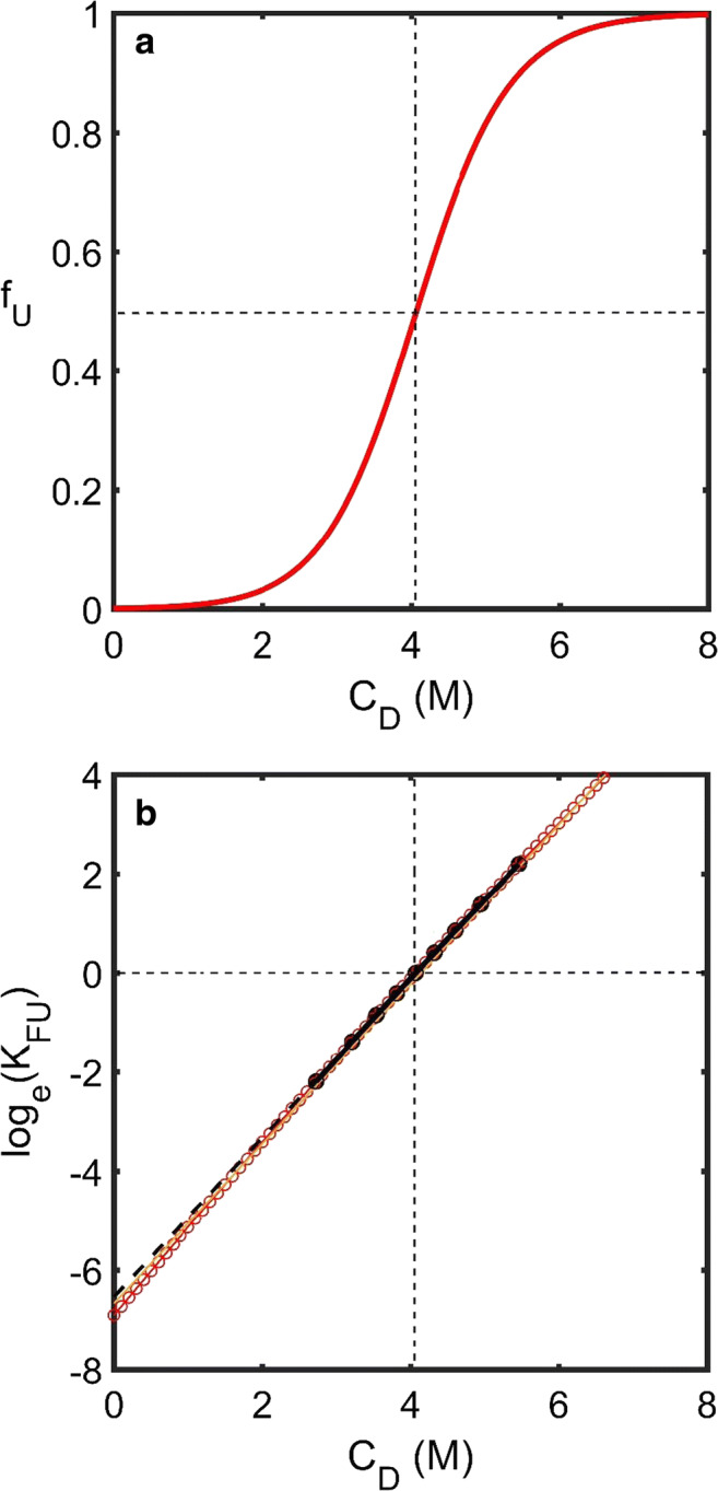
Denaturant-induced unfolding. a Simulated dependence of the fraction of unfolded protein upon denaturant concentration (f_U upon C_D) generated using Eq. 2 which is based upon three parameters, the equilibrium unfolding constant at zero denaturant concentration, ${\left(K_{\mathit{FU}}\right)}_{T_1,P_1,{\left\{n_j\right\}}_0,\left(C_D=0\right)}$, the denaturant site-binding concentration, k_PD, and the difference in total number of denaturant sites available between the unfolded and folded forms of the protein, ΔN_D. Dotted lines indicate the transition midpoint. b A plot of log(K_FU) vs. C_D will be linear around C_D = 0 but not necessarily linear in the transition region. Black-dashed lines are based on an extrapolation of values in the f_U ∈ [0.1, 0.9] region with the extrapolated value at C_D = 0 different from that predicted by Eq. 26 (red circles). (Translated and reprinted with full permission from Wakayama et al. (2019))

$$f_U=\frac{{\left(K_{\mathit{FU}}\right)}_{T_1,P_1,{\left\{n_j\right\}}_0,\left(C_D=0\right)}.{\left(1+k_{\mathit{PD}}{C}_D\right)}^{{\Delta N}_D}}{1+{\left(K_{\mathit{FU}}\right)}_{T_1,P_1,{\left\{n_j\right\}}_0,\left(C_D=0\right)}.{\left(1+k_{\mathit{PD}}{C}_D\right)}^{{\Delta N}_D}}$$ 26

Searching for the causation of linearity in the standard m value-type plot of log_e(K_FU) vs. C_D, we note that taking natural logarithms of both sides of Eq. 25b produces Eq. 27 (Fig. 5b).

$${log}_e{\left(K_{\mathit{FU}}\right)}_{T_1,P_1,{\left\{n_j\right\}}_2,{\left(C_D\right)}_2}{=log}_e{\left(K_{\mathit{FU}}\right)}_{T_1,P_1,{\left\{n_j\right\}}_0,\left(C_D=0\right)}+{\Delta N}_D.{log}_e\left(1+k_{\mathit{PD}}{C}_D\right)$$ 27

For small values of x, the series expansion for $\mathrm{lo}{\mathrm{g}}_e\left(1+\mathrm{x}\right)\approx {\sum }_{i=0}^{\infty }\int {\left(-x\right)}^i.\mathit{dx}$ allows one to write the approximate form at any concentration (C_D)₂ (Eq. 28a) and at a particular reference concentration (C_D)₁ (Eq. 28b).

$${log}_e{\left(K_{\mathit{FU}}\right)}_{T_1,P_1,{\left\{n_j\right\}}_2,{\left(C_D\right)}_2}={log}_e{\left(K_{\mathit{FU}}\right)}_{T_1,P_1,{\left\{n_j\right\}}_0,\left(C_{D=0}\right)}+\Delta N_D\cdot \left[\left(k_{\mathit{PD}}{\left(C_D\right)}_2\right)-\frac{1}{2}.{\left(k_{\mathit{PD}}{\left(C_D\right)}_2\right)}^2+\dots \right]$$ 28a

$${log}_e{\left(K_{\mathit{FU}}\right)}_{T_1,P_1,{\left\{\mathit{nj}\right\}}_1,{\left(C_D\right)}_1}={log}_e{\left(K_{\mathit{FU}}\right)}_{T_1,P_1,{\left\{n_j\right\}}_0,\left(C_{D=0}\right)}+\Delta N_D\cdot \left[\left(k_{\mathit{PD}}{\left(C_D\right)}_1\right)-\frac{1}{2}.{\left(k_{\mathit{PD}}{\left(C_D\right)}_1\right)}^2+\dots \right]$$ 28b

If the reference concentration (C_D)₁ is set at the midpoint (C_D)_mp then (C_U)_mp = (C_F)_mp and ${\left(K_{\mathit{FU}}\right)}_{T_1,P_1,{\left\{n_j\right\}}_1,{\left(C_D\right)}_1}=1.$ Subtracting Eq. 28b from 28a yields Eq. 29.

$${log}_e{\left(K_{\mathit{FU}}\right)}_{T_1,P_1,{\left\{n_j\right\}}_2,{\left(C_D\right)}_2}={\Delta N}_D.\left[\left(k_{\mathit{PD}}\left\{{\left(C_D\right)}_2-{\left(C_D\right)}_{\mathit{mp}}\right\}\right)-\frac{1}{2}.\left\{{\left(k_{\mathit{PD}}{\left(C_D\right)}_2\right)}^2-{\left(k_{\mathit{PD}}{\left(C_D\right)}_{\mathit{mp}}\right)}^2\right\}+\dots \right]$$ 29

Upon initial inspection, it would seem that Eq. 29 suggests an approximate value for the slope around the midpoint of a plot of log_e$\left[{\left(K_{\mathit{FU}}\right)}_{T_1,P_1,{\left\{n_j\right\}}_2,{\left(C_D\right)}_2}\right]$ vs. ΔC_D, of ΔN_D·k_PD. For small perturbations, we may be tempted to define a corresponding m_D value at the midpoint which, according to Eq. 4c, should be given by ΔN_D·R T_mp k_PD. However, for a more complete interpretation, it is important to understand two points, (i) that to achieve the approximate forms (shown in Eq. 28), a Taylor expansion was performed around the point C_D = 0; therefore, the subtracted expression (shown as Eq. 29) involves the difference of two approximations which are themselves increasingly suspect beyond the point C_D = 0, and (ii) the expansion does not progress in ΔC_D but in C_D, i.e., note that the higher order zth terms involve ((C_D)₂)^z − ((C_D)_mp)^z and not ((C_D)₂ − (C_D)_mp)^z. As such, a plot of log_e$\left[{\left(K_{\mathit{FU}}\right)}_{T_1,P_1,{\left\{n_j\right\}}_2,{\left(C_D\right)}_2}\right]$ vs. C_D should be linear about C_D = 0 but not necessarily at the midpoint where this assumption has previously been used as the basis of extrapolation procedures (Pace 1986; Auton and Bolen 2005; Street et al. 2006). That linearity is often observed is due to the extremely small value of k_PD, [1 × 10⁻³ − 1 × 10⁻¹ M⁻¹] measured for the binding of denaturants such as urea and guanidine hydrochloride in aqueous systems (Aune and Tanford 1968; Schellman 2002; Hall et al. 2018). It remains to be seen what magnitude k_PD will take when the denaturant effect arises from preferential solvation of protein by the ionic liquid or by denaturing solutes dissolved within them as opposed to the case for aqueous solvent (Canchi and García 2013; Smiatek 2017). Other complicating factors associated with this approach (such as differential binding of denaturant to folded and unfolded protein states) have been recently explored (Hall et al. 2018).

Conclusions

As discussed by Wakayama et al. (2019), the use of ionic liquids as the base solvent medium in the rational design of enzyme-based catalytic systems represents a point of profound divergence from the entire preceding historical record of enzymatic improvement (Park and Kazlauskas 2003; Itoh 2017). Whether occurring via natural evolution, rational design, or directed-evolution (Kuchner and Arnold 1997; Porter et al. 2016), improvements in enzyme function have previously taken place in aqueous solvent,10 which has constrained the reaction environment in terms of reactant/product solubility, reactant structure, reactant chemical state, and operative temperature range of the solution [typically ~ 0–100 °C]. With physical and chemical properties which can be vastly different from water (Seddon et al. 2000; Kazakov et al. 2018), the use of ionic liquids as the reaction solvent offers the potential to alter the constraints associated with an aqueous reaction environment, thereby opening a door to previously un-thought of possibilities in the field of bio-catalysis (Brogan and Hallett 2016; Schröder 2017; Itoh 2017). Despite the excitement, the catalytic activity of enzymes is still predicated upon the polypeptide chain adopting the necessary three-dimensional structure capable of interacting with reactants to lower the relative free energy of their transition state.11 As such, perhaps the most important factor in the use of ionic liquids to facilitate enzyme-based catalysis is their role in determining protein structure (Takekiyo et al. 2013; Patel et al. 2014; Reslan and Kayser 2018). In this short note, we have provided a brief overview of suitable empirical and theory-based strategies for the assessment of protein structure in response to changes made in either the temperature, pressure, or solvent composition and have attempted to explain the origin of the terms appearing within the analytical expressions.

There are a number of current examples of the use of ionic liquids for the enhancement of the enzyme-catalyzed production of commercially important chemicals (De Diego et al. 2005; Dang et al. 2007; Dabirmanesh et al. 2012; Kumar et al. 2017; Itoh 2017; Meyer et al. 2018). From a standard process engineering viewpoint, the target function for optimization in any commercial venture is the unit cost of production of the chemical product. For the process-design engineer, the alterable variables to achieve this enhancement in production cost are typically the system temperature and pressure, the solvent composition, the reactant concentrations, and the type of catalyst along with its chemical and structural state (Bommarius 2015). Use of ionic liquids as the solvent in enzyme-catalyzed reactions opens new areas of search-space with regard to all of the system variables, including the design and optimization of the enzyme catalyst itself and exploration of the effect of added cosolvents in regulating enzyme behavior (Hall 2002, 2006; Hall and Dobson 2006). Despite the existence of these new horizons, a proper understanding of the enzyme’s protein structure along with its sensitivity to, and competition between, denaturation and aggregation (Constatinescu et al. 2010; Hall 2006) will be a vital component of intelligent scientific and business-based decision-making.

In our attempts to review this field, we were impressed with the large volume of published work. Indeed, the sentiment expressed in the prefatory comments of a recent monograph on ionic liquids (Koel 2009),

Ex sale et sole existunt omnia – From the salt and sun all things come forth,

seems to be apt in at least a few different ways. This review is different from the many others that relate to the use of ionic liquids in biological applications (e.g., see articles within the recent special issue edited by Benedetto and Galla 2018) in that, it has specifically attempted to fill the information gap necessary for the field to move beyond the commonly adopted practice of ranking the stability of proteins in ionic liquids in terms of conditions defining the unfolding midpoint. In this aim, the present review shares a common purpose with the review by Smiatek (2017) although the theoretical approaches are geared to different audiences in the sense that the review by Smiatek is developed using theory largely useful to computational scientists while the current review deals in observables and equations useful for “wet” experimentalists. We hope that the detailed and thermodynamically consistent description of existing assessment strategies presented in this review will be beneficial to those crossing into this bold new frontier of ionic-liquid-enabled enzyme design.

Appendix 1: Thermodynamics of open systems

For an open system (for which we may independently change either the applied pressure, the temperature, or the number/concentration of any of the non-reacting solution components), the difference in free energy between two equilibrium states is given in Eq. A1 (Van Holde et al. 2006a).

$$\mathrm{dG}={\left(\frac{\partial G}{\partial T}\right)}_{P,\left\{n_j\right\}}.\mathit{dT}+{\left(\frac{\partial G}{\partial P}\right)}_{T,\left\{n_j\right\}}.\mathit{dP}+{\sum }_{i=1}^Q{\left(\frac{\partial G}{\partial n_i}\right)}_{T,P,\left\{n_{i\ne j}\right\}}.d{n}_i$$ A1

Each of the partial derivative terms can be evaluated to produce the standard identities shown in Eq. A2,

$${\left(\frac{\partial G}{\partial T}\right)}_{P,\left\{n_j\right\}}=-S_{\text{system}}$$ A2a

$${\left(\frac{\partial G}{\partial P}\right)}_{T,\left\{n_j\right\}}=V_{\text{system}}$$ A2b

$${\left(\frac{\partial G}{\partial n_i}\right)}_{T,P,\left\{n_{i\ne j}\right\}}={\mu }_i={\mu }_i^{°}+\mathit{\text{RTln}}\left(\frac{C_i}{C_i^{°}}\right)$$ A2c

In Eq. A2, S and V are respectively the entropy and volume of the system and μ_i is the change in free energy of the system per fractional change in mole composition of a particular ith type of chemical component (and furthermore μ_i^° is the change in free energy per fractional change in mole composition of the ith type of chemical component when the concentration of that component is at its standard state concentration C_i^° typically a concentration of 1 M). Upon substitution of these identities into Eq. A1, we obtain Eq. A3,

$$\mathrm{dG}=-{\mathrm{S}}_{\text{system}}.\mathit{dT}+{\mathrm{V}}_{\text{system}}.\mathit{dP}+{\sum }_{j=1}^Q{\mu }_j.d{n}_j$$ A3

Importantly, Eq. A3 describes a change in free energy in terms of partial differentials with Q + 2 independent variables (where Q is the number of independently variable chemical components). If a change is made to the system, the overall change in free energy, dG, can be calculated through a basic book-keeping exercise according to Eq. A3 with each partial derivative evaluated in turn with independent variables updated as required for evaluation of a state variable. For a situation in which the temperature, pressure, and number of particles of a component can be reversibly altered, the derivative of the difference in free energy of the system with respect to the molar composition of the ith component is given by Eq. A4a. Upon realizing that the order of differentiation does not matter, we may re-express, $\frac{d\left(\mathit{dG}\right)}{d{n}_i}$, as the incremental change in chemical potential, dμ_i, and likewise denote the various component terms in Eq. A4a as representing constrained partial changes of the chemical potential, ∂μ_i, under the condition that dn_j = 0 for all components j ≠ i (Eq. A4b). The result described by Eq. A4b can be used to calculate the chemical potential of component i at a new set of conditions according to Eq. A4c.

$${\frac{d\left(\mathit{dG}\right)}{d{n}_i}}_{T_1,P_1,{\left\{n_i\right\}}_1\to T_2,P_2,{\left\{n_i\right\}}_2}=-{\left(\frac{\mathrm{\partial S}}{\partial n_i}\right)}_{T,P,\left\{n_j\right\}}.\mathit{dT}+{\left(\frac{\mathrm{\partial V}}{\partial n_i}\right)}_{T,P,\left\{n_j\right\}}.\mathit{dP}+{\sum }_{j=1}^Q{\left(\frac{\partial {\mu }_j}{\partial n_i}\right)}_{{\left(n_i\right)}_1\to {\left(n_i\right)}_2;T,P,\left\{n_{i\ne k}\right\}}.d{n}_j$$ A4a

$${\left(d{\mu }_i\right)}_{T_1,P_1,{\left\{n_i\right\}}_1\to T_2,P_2,{\left\{n_i\right\}}_2}={\left(\partial {\mu }_i\right)}_{T_1\to T_2;P,\left\{n_{j\ne i}\right\}}+{\left(\partial {\mu }_i\right)}_{P_1\to P_2;T,\left\{n_{j\ne i}\right\}}+{\left(\partial {\mu }_i\right)}_{{\left(n_i\right)}_1\to {\left(n_i\right)}_2;T,P,\left\{n_{j\ne i}\right\}}$$ A4b

$${\left({\mu }_i\right)}_{T_2,P_2,{\left\{n_j\right\}}_2}={\left({\mu }_i\right)}_{T_1,P_1,{\left\{n_j\right\}}_1}+{\left(d{\mu }_i\right)}_{T_1,P_1,{\left\{n_j\right\}}_1\to T_2,P_2,{\left\{n_j\right\}}_2}$$ A4c

Systems at equilibrium and the definition of equilibrium constants

At constant temperature and pressure, Eq. A3 collapses to A5a. We may simplify Eq. A5a on the condition of chemical components participating in a chemical equilibrium. If components A and B exist in chemical equilibrium, such that, A ⇌ B12 then we may express change in terms of a reaction progress variable ξ such that dξ = |dn_A| = |dn_B| (Eq. A5b). Differentiation with respect to the reaction progress variable produces Eq. A5c.

$$\mathrm{dG}={\sum }_{i=1}^Q{\mu }_i.d{n}_i$$ A5a

$$\mathrm{dG}={\mu }_B.\mathit{d\xi }-{\mu }_A.\mathit{d\xi }$$ A5b

$$\frac{\mathit{dG}}{\mathit{d\xi }}=∆{\mu }_{\mathit{AB}}$$ A5c

Equation A5c defines the condition for equilibrium in the sense that the reaction will proceed until the differential described in Eq. A5c is located at a minima, i.e., $\frac{\mathit{dG}}{\mathit{d\xi }}=0$, from which Eq. A6 follows,

$$∆{\mu }_{\mathit{AB}}=0$$ A6a

$${\left({\mu }_A\right)}_{T_1,P_1,{\left\{n_{j\ne A}\right\}}_1}={\left({\mu }_B\right)}_{T_1,P_1,{\left\{n_{j\ne B}\right\}}_1}$$ A6b

Inserting the equation for the definition of the chemical potential from Eq. A2c yields Eq. A7.

$${\left({\mu }_A^{°}\right)}_{T_1,P_1,{\left\{n_{j\ne A}\right\}}_1}+R{T}_1\mathit{ln}\left(\frac{{\left(C_A\right)}_1}{C_A^{\circ }}\right)={\left({\mu }_B^{°}\right)}_{T_1,P_1,{\left\{n_{j\ne B}\right\}}_1}+R{T}_1\mathit{ln}\left(\frac{{\left(C_B\right)}_1}{C_B^{\circ }}\right)$$ A7

From which it follows,

$$-R{T}_1\mathit{ln}\left(\frac{{\left(C_B\right)}_1.C_A^{\circ }}{{\left(C_A\right)}_1.C_B^{\circ }}\right)={\left({\mu }_B^{°}\right)}_{T_1,P_1,{\left\{n_{j\ne B}\right\}}_1}-{\left({\mu }_A^{°}\right)}_{T_1,P_1,{\left\{n_{j\ne A}\right\}}_1}$$ A8a

$${\left({\mathrm{K}}_{\mathit{AB}}\right)}_{T_1,P_1,{\left\{n_j\right\}}_1}=\left(\frac{{\left(C_B\right)}_1.C_A^{\circ }}{{\left(C_A\right)}_1.C_B^{\circ }}\right)=exp\left(\frac{-\left[{\left({\mu }_B^{°}\right)}_{T_1,P_1,{\left\{n_j\ne B\right\}}_1}-{\left({\mu }_A^{°}\right)}_{T_1,P_1{\left\{n_{j\ne A}\right\}}_1}\right]}{R{T}_1}\right)$$ A8b

Calculating equilibrium constants at a new set of conditions

To understand how the equilibrium constant may change with changing conditions, it is important to realize that at any altered set of conditions (say T₂, P₂, {n_j}₂), we may express the equilibrium condition at constant temperature and pressure in an identical manner to Eq. A8b (Eq. A9).

$${\left({\mathrm{K}}_{\mathit{AB}}\right)}_{T_2,P_2,{\left\{n_j\right\}}_2}=\left(\frac{{\left(C_B\right)}_1.C_A^{\circ }}{{\left(C_A\right)}_1.C_B^{\circ }}\right)=exp\left(\frac{-\left[{\left({\mu }_B^{°}\right)}_{T_2,P_2,{\left\{n_j\ne B\right\}}_2}-{\left({\mu }_A^{°}\right)}_{T_2,P_2,{\left\{n_{j\ne A}\right\}}_2}\right]}{R{T}_2}\right)$$ A9

We can relate the chemical potential of components A and B defined at a new set of conditions (T₂, P₂, {n_j}₂) to their chemical potentials defined under a previous set of conditions (T₁, P₁, {n_j}₁) by use of the equation for the total differential given in A4b (Eq. A10).

$${\left({\mu }_A\right)}_{T_2,P_2,{\left\{n_{j\ne A}\right\}}_2}={\left({\mu }_A\right)}_{T_1,P_1,{\left\{n_{j\ne A}\right\}}_1}+{\left(d{\mu }_A\right)}_{T_1,P_1,{\left\{n_j\right\}}_1\to T_2,P_2,{\left\{n_j\right\}}_2}$$ A10a

$${\left({\mu }_B\right)}_{T_2,P_2,{\left\{n_{j\ne B}\right\}}_2}={\left({\mu }_B\right)}_{T_1,P_1,{\left\{n_{j\ne B}\right\}}_1}+{\left(d{\mu }_B\right)}_{T_1,P_1,{\left\{n_j\right\}}_1\to T_2,P_2,{\left\{n_j\right\}}_2}$$ A10b

Inserting the result for Eq. A2c into Eq. A10, we have the condition for equilibrium after some change is made in temperature, pressure, or composition to a system at equilibrium (Eq. A11).

$${\left({\mu }_A^{°}\right)}_{T_1,P_1,{\left\{n_{j\ne A}\right\}}_1}+R{T}_1\mathit{ln}\left(\frac{{\left(C_A\right)}_1}{C_A^{\circ }}\right)+{\left(d{\mu }_A\right)}_{T_1,P_1,{\left\{n_j\right\}}_1\to T_2,P_2,{\left\{n_j\right\}}_2}={\left({\mu }_B^{°}\right)}_{T_1,P_1,{\left\{n_{j\ne B}\right\}}_1}+R{T}_1\mathit{ln}\left(\frac{{\left(C_B\right)}_1}{C_B^{\circ }}\right)+{\left(d{\mu }_B\right)}_{T_1,P_1,{\left\{n_j\right\}}_1\to T_2,P_2,{\left\{n_j\right\}}_2}$$ A11

In the main paper, we utilize Eq. A11 to derive analytical relations for the change in extent of protein unfolding with changes in environmental conditions.

Definition of equilibrium constants for the denaturant binding mechanism

To derive a set of equations which account for successive denaturant binding to various “sites” on the protein, we first develop the case for the reversible binding of denaturant to a specific site and then later relax the requirement for site specificity, to include the statistically degenerate case in which each site is considered equivalent. For interaction between a specific protein site and denaturant molecule (P_site + D ⇌ P_siteD), the condition for the site-binding equilibrium and the site-binding equilibrium constant, ${\left(k_{P_{\text{site}}D}\right)}_{T_1,P_1,{\left\{n_j\right\}}_1,{\left(C_D\right)}_1}$, are respectively given in Eq. A12a and b.

$${\mathrm{\mu }}_{P_{\mathit{\text{site}}}}+{\mathrm{\mu }}_D={\mathrm{\mu }}_{P_{\text{site}}D}$$ A12a

$${\left(k_{P_{\mathit{\text{site}}}D}\right)}_{T_1,P_1,{\left\{n_j\right\}}_1,{\left(C_D\right)}_1}=exp\left(\frac{-\left[{\mathrm{\mu }}_{P_{\mathit{\text{site}}}D}^{°}-\left({\mathrm{\mu }}_{P_{\mathit{\text{site}}}}^{°}+{\mathrm{\mu }}_D^{°}\right)\right]}{R{T}_1}\right)=\frac{C_{\mathit{PD}}}{C_{P_{\mathit{\text{site}}}}.{\left(C_D\right)}_1}$$ A12b

If there are multiple ways of configuring a particular jth loading state of denaturant on the protein molecule, $C_{P{D}_j}$, then the site-binding constant must be modified by a statistical factor, $F_{P{D}_j}$, which accounts for all of the different possible ways that the PD_j state can be constructed, Eq. A13a. Incorporating this degeneracy into the equilibrium defines the relationship between the operative equilibrium constant,${\left({\mathrm{K}}_{P{D}_j}\right)}_{T_1,P_1,{\left\{n_j\right\}}_1,{\left(C_D\right)}_1}$, and the site-binding equilibrium constant, ${\left(k_{P_{\text{site}}D}\right)}_{T_1,P_1,{\left\{n_j\right\}}_1,{\left(C_D\right)}_1}$, Eq. A13b (Hall et al. 2018).

$${\mathrm{C}}_{P{D}_j}=F_{P{D}_j}.C_{P_{\text{site}}D}$$ A13a

$${\left({\mathrm{K}}_{P{D}_j}\right)}_{T_1,P_1,{\left\{n_j\right\}}_1,{\left(C_D\right)}_1}=\frac{C_{P{D}_j}}{C_{P{D}_{j-1}}.{\left(C_D\right)}_1}=\frac{F_{P{D}_j}.C_{P_{\text{site}}D}}{F_{P{D}_{j-1}}.C_{P_{\text{site}}}.{\left(C_D\right)}_1}=\left(\frac{F_{P{D}_j}}{F_{P{D}_{j-1}}}\right).{\left(k_{P_{\text{site}}D}\right)}_{T_1,P_1,{\left\{n_j\right\}}_1,{\left(C_D\right)}_1}$$ A13b

For j denaturant molecules loaded onto a protein with a total of N_PD equivalent and indistinguishable sites, the statistical factor, $F_{P{D}_j}$, is given by Eq. A14 (which readers will note is functionally equivalent to Eq. 24c and d provided in the main text).

$$F_{P{D}_j}=\frac{N_{\mathit{PD}}!}{\left(N_{\mathit{PD}}-j\right)!.j!}$$ A14

Summation of all forms of protein-denaturant complex yields Eq. A15a. Using Eq. A13b and Eq. A15a may be expressed in an equivalent form known as the binding polynomial, Eq. A15b (Van Holde et al. 2006b).

$${\left(C_P\right)}_{\text{TOTAL}}={\sum }_{i=0}^{\infty }{C}_{P{D}_i}$$ A15a

$${\left(C_P\right)}_{\text{TOTAL}}={\left(C_P\right)}_1.{\sum }_{i=0}^{\infty }{F}_{P{D}_i}.{\left({\mathrm{k}}_{P_{\text{site}}D}.{\left(C_D\right)}_1\right)}^i$$ A15b

If additional consideration is given to the two different F and U forms of the protein, we may use the result given in Eq. A15b to produce an operative equilibrium constant of a type identical to that given in Eq. 25.

Compliance with ethical standards

Funding information

The work of DH was jointly supported by funds and resources associated with an Australian National University (ANU) Senior Research Fellowship, a Guest Associate Professor position at the Institute for Protein Research, Osaka University and a short term fellowship at the Laboratory of Biochemistry and Genetics of the NIH (NIDDK) in August of 2018. The receipt of a TOBITATE exchange program grant funded a 1-year exchange for RW to ANU. TOBITATE was funded by the Japan National Exchange Program part of the Ministry of Education, Culture Science and Technology (MEXT) of Japan.

Conflict of interest

Ryota Wakayama declares that he has no conflict of interest. Susumu Uchiyama declares that he has no conflict of interest. Damien Hall declares that he has no conflict of interest.

Ethical approval

This article does not contain any studies with human participants or animals performed by any of the authors.

References

- Anfinsen CB. Principles that govern the folding of protein chains. Science. 1973;181:223–230. doi: 10.1126/science.181.4096.223. [DOI] [PubMed] [Google Scholar]
- Aparicio S, Atilhan M, Karadas F. Thermophysical properties of pure ionic liquids: review of present situation. Ind Eng Chem Res. 2010;49(20):9580–9595. doi: 10.1021/ie101441s. [DOI] [Google Scholar]
- Aune KC, Tanford C. Thermodynamics of the denaturation of lysozyme by guanidine hydrochloride. II. Dependence on denaturant concentration at 25. Biochemistry. 1969;8(11):4586–4590. doi: 10.1021/bi00839a053. [DOI] [PubMed] [Google Scholar]
- Auton M, Bolen DW. Predicting the energetics of osmolyte-induced protein folding/unfolding. Proc Natl Acad Sci. 2005;102:15065–15068. doi: 10.1073/pnas.0507053102. [DOI] [PMC free article] [PubMed] [Google Scholar]
- Becktel WJ, Schellman JA. Protein stability curves. Biopolymers: Original Research on Biomolecules. 1987;26(11):1859–1877. doi: 10.1002/bip.360261104. [DOI] [PubMed] [Google Scholar]
- Benedetto A, Galla HJ. Editorial of the “ionic liquids and biomolecules” special issue. Biophys Rev. 2018;9(3):1–4. doi: 10.1007/s12551-018-0426-3. [DOI] [PMC free article] [PubMed] [Google Scholar]
- Bommarius AS. Biocatalysis: a status report. Ann Rev Chem Biomol Eng. 2015;6:319–345. doi: 10.1146/annurev-chembioeng-061114-123415. [DOI] [PubMed] [Google Scholar]
- Brogan AP, Hallett JP. Solubilizing and stabilizing proteins in anhydrous ionic liquids through formation of protein–polymer surfactant nanoconstructs. J Am Chem Soc. 2016;138(13):4494–4501. doi: 10.1021/jacs.5b13425. [DOI] [PubMed] [Google Scholar]
- Canchi DR, García AE. Cosolvent effects on protein stability. Annu Rev Phys Chem. 2013;64:273–293. doi: 10.1146/annurev-physchem-040412-110156. [DOI] [PubMed] [Google Scholar]
- Chi EY, Krishnan S, Randolph TW, Carpenter JF. Physical stability of proteins in aqueous solution: mechanism and driving forces in nonnative protein aggregation. Pharm Res. 2003;20(9):1325–1336. doi: 10.1023/A:1025771421906. [DOI] [PubMed] [Google Scholar]
- Chum HL, Koch VR, Miller LL, Osteryoung RA. Electrochemical scrutiny of organometallic iron complexes and hexamethylbenzene in a room temperature molten salt. J Am Chem Soc. 1975;97(11):3264–3265. doi: 10.1021/ja00844a081. [DOI] [Google Scholar]
- Constantinescu D, Weingärtner H, Herrmann C. Protein denaturation by ionic liquids and the Hofmeister series: a case study of aqueous solutions of ribonuclease a. Angew Chem Int Ed. 2007;46(46):8887–8889. doi: 10.1002/anie.200702295. [DOI] [PubMed] [Google Scholar]
- Constatinescu D, Herrmann C, Weingärtner H. Patterns of protein unfolding and protein aggregation in ionic liquids. Phys Chem Chem Phys. 2010;12(8):1756–1763. doi: 10.1039/b921037g. [DOI] [PubMed] [Google Scholar]
- Dabirmanesh B, Khajeh K, Ranjbar B, Ghazi F, Heydari A. Inhibition mediated stabilization effect of imidazolium based ionic liquids on alcohol dehydrogenase. J Mol Liq. 2012;170:66–71. doi: 10.1016/j.molliq.2012.03.004. [DOI] [Google Scholar]
- Dang DT, Ha SH, Lee SM, Chang WJ, Koo YM. Enhanced activity and stability of ionic liquid-pretreated lipase. J Mol Catal B Enzym. 2007;45(3–4):118–121. doi: 10.1016/j.molcatb.2007.01.001. [DOI] [Google Scholar]
- De Diego T, Lozano P, Gmouh S, Vaultier M, Iborra JL. Understanding structure− stability relationships of Candida antartica Lipase B in ionic liquids. Biomacromolecules. 2005;6(3):1457–1464. doi: 10.1021/bm049259q. [DOI] [PubMed] [Google Scholar]
- Dill KA. Theory for the folding and stability of globular proteins. Biochemistry. 1985;24(6):1501–1509. doi: 10.1021/bi00327a032. [DOI] [PubMed] [Google Scholar]
- Dill KA, MacCallum JL. The protein-folding problem, 50 years on. Science. 2012;338(6110):1042–1046. doi: 10.1126/science.1219021. [DOI] [PubMed] [Google Scholar]
- Domańska U (2009). General review of ionic liquids and their properties. Chapter 1 of “Analytical Chemistry: ionic liquids in chemical analysis’ (Ed. Koel, M). p. 1–71
- Eftink MR, Ionescu R. Thermodynamics of protein unfolding: questions pertinent to testing the validity of the two-state model. Biophys Chem. 1997;64(1–3):175–197. doi: 10.1016/S0301-4622(96)02237-5. [DOI] [PubMed] [Google Scholar]
- Fersht A (1999). A guide to enzyme catalysis and protein folding. Structure and Mechanism in Protein Science, “Protein Stability”, New York, W.H. Freeman Press, pp. 508–539 Chapter 17
- Fields PA. Protein function at thermal extremes: balancing stability and flexibility. Comp Biochem Physiol A Mol Integr Physiol. 2001;129(2–3):417–431. doi: 10.1016/S1095-6433(00)00359-7. [DOI] [PubMed] [Google Scholar]
- Greene RF, Pace CN. Urea and guanidine hydrochloride denaturation of ribonuclease, lysozyme, α-chymotrypsin, and β-lactoglobulin. J Biol Chem. 1974;249:5388–5393. doi: 10.1016/S0021-9258(20)79739-5. [DOI] [PubMed] [Google Scholar]
- Hall D. On the role of the macromolecular phase transitions in biology in response to change in solution volume or macromolecular composition: action as an entropy buffer. Biophys Chem. 2002;98(3):233–248. doi: 10.1016/S0301-4622(02)00072-8. [DOI] [PubMed] [Google Scholar]
- Hall D. The effects of tubulin denaturation on the characterization of its polymerization behavior. Biophys Chem. 2003;104(3):655–682. doi: 10.1016/S0301-4622(03)00040-1. [DOI] [PubMed] [Google Scholar]
- Hall D. Protein self-association in the cell: a mechanism for fine tuning the level of macromolecular crowding? Eur Biophys J. 2006;35(3):276–280. doi: 10.1007/s00249-005-0016-8. [DOI] [PubMed] [Google Scholar]
- Hall D (2012) Semi-automated methods for simulation and measurement of amyloid fiber distributions obtained from transmission electron microscopy experiments. Anal Biochem 421(1):262–277 [DOI] [PubMed]
- Hall D, Dobson CM. Expanding to fill the gap: a possible role for inert biopolymers in regulating the extent of the ‘macromolecular crowding’effect. FEBS Lett. 2006;580(11):2584–2590. doi: 10.1016/j.febslet.2006.04.005. [DOI] [PubMed] [Google Scholar]
- Hall D, Edskes H. Silent prions lying in wait: a two-hit model of prion/amyloid formation and infection. J Mol Biol. 2004;336(3):775–786. doi: 10.1016/j.jmb.2003.12.004. [DOI] [PubMed] [Google Scholar]
- Hall D, Edskes H. A model of amyloid's role in disease based on fibril fracture. Biophys Chem. 2009;145(1):17–28. doi: 10.1016/j.bpc.2009.08.004. [DOI] [PMC free article] [PubMed] [Google Scholar]
- Hall D, Edskes H. Computational modeling of the relationship between amyloid and disease. Biophys Rev. 2012;4(3):205–222. doi: 10.1007/s12551-012-0091-x. [DOI] [PMC free article] [PubMed] [Google Scholar]
- Hall D, Hirota N. Multi-scale modelling of amyloid formation from unfolded proteins using a set of theory derived rate constants. Biophys Chem. 2009;140(1–3):122–128. doi: 10.1016/j.bpc.2008.11.013. [DOI] [PubMed] [Google Scholar]
- Hall D, Huang L. On the use of size exclusion chromatography for the resolution of mixed amyloid aggregate distributions: I. Equilibrium partition models. Anal Biochem. 2012;426(1):69–85. doi: 10.1016/j.ab.2012.04.001. [DOI] [PubMed] [Google Scholar]
- Hall D, Kinjo A, Goto Y. A new look at an old view of denaturant induced protein unfolding. Anal Biochem. 2018;542:40–57. doi: 10.1016/j.ab.2017.11.011. [DOI] [PubMed] [Google Scholar]
- Horinek D, Netz RR. Can simulations quantitatively predict peptide transfer free energies to urea solutions? Thermodynamic concepts and force field limitations. J Phys Chem A. 2011;115(23):6125–6136. doi: 10.1021/jp1110086. [DOI] [PubMed] [Google Scholar]
- Hurley FH, Wier TP. The electrodeposition of aluminium from non-aqueous solutions at room temperature. J Electrochem Soc. 1951;98:207–212. doi: 10.1149/1.2778133. [DOI] [Google Scholar]
- Itoh T. Ionic liquids as tool to improve enzymatic organic synthesis. Chem Rev. 2017;117(15):10567–10607. doi: 10.1021/acs.chemrev.7b00158. [DOI] [PubMed] [Google Scholar]
- Jacquemin J, Husson P, Mayer V, Cibulka I. High-pressure volumetric properties of imidazolium-based ionic liquids: effect of the anion. J Chem Eng Data. 2007;52(6):2204–2211. doi: 10.1021/je700224j. [DOI] [Google Scholar]
- Jaspe J, Hagen SJ. Do protein molecules unfold in a simple shear flow? Biophys J. 2006;91(9):3415–3424. doi: 10.1529/biophysj.106.089367. [DOI] [PMC free article] [PubMed] [Google Scholar]
- Johnson CM, Fersht AR. Protein stability as a function of denaturant concentration: the thermal stability of barnase in the presence of urea. Biochemistry. 1995;34(20):6795–6804. doi: 10.1021/bi00020a026. [DOI] [PubMed] [Google Scholar]
- Kamal MZ, Kumar V, Satyamurthi K, Das KK, Rao NM. Mutational probing of protein aggregates to design aggregation-resistant proteins. FEBS open bio. 2016;6(2):126–134. doi: 10.1002/2211-5463.12003. [DOI] [PMC free article] [PubMed] [Google Scholar]
- Kazakov, A, Magee JW, Chirico RD, Paulechka E, Diky V, Muzny CD, Kroenlein K, and Frenkel M (2018) “NIST standard reference database 147: NIST ionic liquids database - (ILThermo)”, Version 2.0, National Institute of Standards and Technology, Gaithersburg MD, 20899, http://ilthermo.boulder.nist.gov.
- Koel M (2009). Introduction to ‘Analytical Chemistry: ionic liquids in chemical analysis’ (Ed. Koel, M). p. xxvii–xxxi
- Kuchner O, Arnold FH. Directed evolution of enzyme catalysts. Trends Biotechnol. 1997;15(12):523–530. doi: 10.1016/S0167-7799(97)01138-4. [DOI] [PubMed] [Google Scholar]
- Kumar PK, Jha I, Venkatesu P, Bahadur I, Ebenso EE. A comparative study of the stability of stem bromelain based on the variation of anions of imidazolium-based ionic liquids. J Mol Liq. 2017;246:178–186. doi: 10.1016/j.molliq.2017.09.037. [DOI] [Google Scholar]
- Lesch V, Heuer A, Tatsis VA, Holm C, Smiatek J (2015) Peptides in the presence of aqueous ionic liquids: tunable co-solutes as denaturants or protectants? Phys Chem Chem Phys 17(39):26049–26053 [DOI] [PubMed]
- Lima-Ramos J, Neto W, Woodley JM. Engineering of biocatalysts and biocatalytic processes. Top Catal. 2014;57(5):301–320. doi: 10.1007/s11244-013-0185-0. [DOI] [Google Scholar]
- Marsh KN, Boxall JA, Lichtenthaler R. Room temperature ionic liquids and their mixtures—a review. Fluid Phase Equilib. 2004;219(1):93–98. doi: 10.1016/j.fluid.2004.02.003. [DOI] [Google Scholar]
- McPhie P, Ni YS, Minton AP. Macromolecular crowding stabilizes the molten globule form of apomyoglobin with respect to both cold and heat unfolding. J Mol Biol. 2006;361(1):7–10. doi: 10.1016/j.jmb.2006.05.075. [DOI] [PubMed] [Google Scholar]
- Meyer LE, von Langermann J, Kragl U. Recent developments in biocatalysis in multiphasic ionic liquid reaction systems. Biophys Rev. 2018;10:1–10. doi: 10.1007/s12551-018-0423-6. [DOI] [PMC free article] [PubMed] [Google Scholar]
- Mezzenga R, Fischer P. The self-assembly, aggregation and phase transitions of food protein systems in one, two and three dimensions. Rep Prog Phys. 2013;76(4):046601. doi: 10.1088/0034-4885/76/4/046601. [DOI] [PubMed] [Google Scholar]
- Mozhaev VV, Heremans K, Frank J, Masson P, Balny C. High pressure effects on protein structure and function. Proteins-Struct Funct Genet. 1996;24(1):81–91. doi: 10.1002/(SICI)1097-0134(199601)24:1<81::AID-PROT6>3.0.CO;2-R. [DOI] [PubMed] [Google Scholar]
- Myers JK, Pace CN, Scholtz JM. Denaturant m values and heat capacity changes: relation to changes in accessible surface areas of protein unfolding. Protein Sci. 1995;4(10):2138–2148. doi: 10.1002/pro.5560041020. [DOI] [PMC free article] [PubMed] [Google Scholar]
- Naushad M, Al-Othman ZA, Khan AB, Ali M. Effect of ionic liquid on activity, stability, and structure of enzymes: a review. Int J Biol Macromol. 2012;51(4):555–560. doi: 10.1016/j.ijbiomac.2012.06.020. [DOI] [PubMed] [Google Scholar]
- Nicholson EM, Scholtz JM. Conformational stability of the Escherichia coli HPr protein: test of the linear extrapolation method and a thermodynamic characterization of cold denaturation. Biochemistry. 1996;35(35):11369–11378. doi: 10.1021/bi960863y. [DOI] [PubMed] [Google Scholar]
- O’Brien EP, Brooks BR, Thirumalai D. Molecular origin of constant m-values, denatured state collapse, and residue-dependent transition midpoints in globular proteins. Biochemistry. 2009;48(17):3743–3754. doi: 10.1021/bi8021119. [DOI] [PMC free article] [PubMed] [Google Scholar]
- Oberhauser AF, Hansma PK, Carrion-Vazquez M, Fernandez JM. Stepwise unfolding of titin under force-clamp atomic force microscopy. Proc Natl Acad Sci. 2001;98(2):468–472. doi: 10.1073/pnas.98.2.468. [DOI] [PMC free article] [PubMed] [Google Scholar]
- Pace CN, (1986). Determination and analysis of urea and guanidine hydrochloride denaturation curves. In Methods in enzymology (Vol. 131, pp. 266–280). Academic Press [DOI] [PubMed]
- Pace CN, Shaw KL. Linear extrapolation method of analyzing solvent denaturation curves. Proteins: Structure, Function, and Bioinformatics. 2000;41(S4):1–7. doi: 10.1002/1097-0134(2000)41:4+<1::AID-PROT10>3.0.CO;2-2. [DOI] [PubMed] [Google Scholar]
- Pandharipande PP, Makhatadze GI. Applications of pressure perturbation calorimetry to study factors contributing to the volume changes upon protein unfolding. Biochimica Biophysica Acta (BBA)-General Subj. 2016;1860(5):1036–1042. doi: 10.1016/j.bbagen.2015.08.021. [DOI] [PubMed] [Google Scholar]
- Park S, Kazlauskas RJ. Biocatalysis in ionic liquids–advantages beyond green technology. Curr Opin Biotechnol. 2003;14(4):432–437. doi: 10.1016/S0958-1669(03)00100-9. [DOI] [PubMed] [Google Scholar]
- Patel R, Kumari M, Khan AB. Recent advances in the applications of ionic liquids in protein stability and activity: a review. Appl Biochem Biotechnol. 2014;172(8):3701–3720. doi: 10.1007/s12010-014-0813-6. [DOI] [PubMed] [Google Scholar]
- Pfeil W, (2012). Protein stability and folding supplement 1: a collection of thermodynamic data. Springer Science & Business Media
- Porter JL, Rusli RA, Ollis DL. Directed evolution of enzymes for industrial biocatalysis. ChemBioChem. 2016;17(3):197–203. doi: 10.1002/cbic.201500280. [DOI] [PubMed] [Google Scholar]
- Privalov PL (2007) Thermodynamic problems in structural molecular biology. Pure Appl Chem 79(8):1445–1462
- Privalov PL, Khechinashvili NN. A thermodynamic approach to the problem of stabilization of globular protein structure: a calorimetric study. J Mol Biol. 1974;86(3):665–684. doi: 10.1016/0022-2836(74)90188-0. [DOI] [PubMed] [Google Scholar]
- Reetz MT, Soni P, Fernandez L, Gumulya Y, Carballeira JD (2010) Increasing the stability of an enzyme toward hostile organic solvents by directed evolution based on iterative saturation mutagenesis using the B-FIT method. Chem Commun 46(45):8657–8658 [DOI] [PubMed]
- Reslan, M. and Kayser, V., (2018). Ionic liquids as biocompatible stabilizers of proteins. Biophys Rev pp1–13 [DOI] [PMC free article] [PubMed]
- Roberts CJ. Non-native protein aggregation kinetics. Biotechnol Bioeng. 2007;98(5):927–938. doi: 10.1002/bit.21627. [DOI] [PubMed] [Google Scholar]
- Rogers TA, Bommarius AS. Utilizing simple biochemical measurements to predict lifetime output of biocatalysts in continuous isothermal processes. Chem Eng Sci. 2010;65(6):2118–2124. doi: 10.1016/j.ces.2009.12.005. [DOI] [PMC free article] [PubMed] [Google Scholar]
- Santoro MM, Bolen DW. Unfolding free energy changes determined by the linear extrapolation method. 1. Unfolding of phenylmethanesulfonyl. alpha-chymotrypsin using different denaturants. Biochemistry. 1988;27(21):8063–8068. doi: 10.1021/bi00421a014. [DOI] [PubMed] [Google Scholar]
- Sasahara K, Sakurai M, Nitta K. Pressure effect on denaturant-induced unfolding of hen egg white lysozyme. Proteins Struct Funct Bioinforma. 2001;44(3):180–187. doi: 10.1002/prot.1083. [DOI] [PubMed] [Google Scholar]
- Satish L, Rana S, Arakha M, Rout L, Ekka B, Jha S, Dash P, Sahoo H. Impact of imidazolium-based ionic liquids on the structure and stability of lysozyme. Spectrosc Lett. 2016;49(6):383–390. doi: 10.1080/00387010.2016.1167089. [DOI] [Google Scholar]
- Schellman JA. The stability of hydrogen-bonded peptide structures in aqueous solution. C R Trav Lab Carlsb Ser Chim. 1956;29:230–259. [PubMed] [Google Scholar]
- Schellman JA. Fifty years of solvent denaturation. Biophys Chem. 2002;96(2–3):91–101. doi: 10.1016/S0301-4622(02)00009-1. [DOI] [PubMed] [Google Scholar]
- Schröder C. Proteins in ionic liquids: current status of experiments and simulations. Top Curr Chem. 2017;375(2):25. doi: 10.1007/s41061-017-0110-2. [DOI] [PMC free article] [PubMed] [Google Scholar]
- Seddon KR, Stark A, Torres MJ. Influence of chloride, water, and organic solvents on the physical properties of ionic liquids. Pure Appl Chem. 2000;72(12):2275–2287. doi: 10.1351/pac200072122275. [DOI] [Google Scholar]
- Sheldon R. Catalytic reactions in ionic liquids. Chem Commun. 2001;23:2399–2407. doi: 10.1039/b107270f. [DOI] [PubMed] [Google Scholar]
- Shiao DF, Lumry R, Fahey J. Chymotrypsinogen family of proteins. XI. Heat-capacity changes accompanying reversible thermal unfolding of proteins. J Am Chem Soc. 1971;93(8):2024–2035. doi: 10.1021/ja00737a030. [DOI] [PubMed] [Google Scholar]
- Smiatek J. Aqueous ionic liquids and their effects on protein structures: an overview on recent theoretical and experimental results. J Phys Condens Matter. 2017;29:233001. doi: 10.1088/1361-648X/aa6c9d. [DOI] [PubMed] [Google Scholar]
- Stefani M, Dobson CM. Protein aggregation and aggregate toxicity: new insights into protein folding, misfolding diseases and biological evolution. J Mol Med. 2003;81(11):678–699. doi: 10.1007/s00109-003-0464-5. [DOI] [PubMed] [Google Scholar]
- Stevenson BJ, Liu JW, Ollis DL. Directed evolution of yeast pyruvate decarboxylase 1 for attenuated regulation and increased stability. Biochemistry. 2008;47(9):3013–3025. doi: 10.1021/bi701858u. [DOI] [PubMed] [Google Scholar]
- Street TO, Bolen DW, Rose GD. A molecular mechanism for osmolyte-induced protein stability. Proc Natl Acad Sci. 2006;103:13997–14002. doi: 10.1073/pnas.0606236103. [DOI] [PMC free article] [PubMed] [Google Scholar]
- Sturtevant JM. Heat capacity and entropy changes in processes involving proteins. Proc Natl Acad Sci. 1977;74(6):2236–2240. doi: 10.1073/pnas.74.6.2236. [DOI] [PMC free article] [PubMed] [Google Scholar]
- Suarez PA, Selbach VM, Dullius JE, Einloft S, Piatnicki CM, Azambuja DS, de Souza RF, Dupont J. Enlarged electrochemical window in dialkyl-imidazolium cation based room-temperature air and water-stable molten salts. Electrochim Acta. 1997;42(16):2533–2535. doi: 10.1016/S0013-4686(96)00444-6. [DOI] [Google Scholar]
- Takekiyo T, Koyama Y, Yamazaki K, Abe H, Yoshimura Y. Ionic liquid-induced formation of the α-helical structure of β-lactoglobulin. J Phys Chem B. 2013;117(35):10142–10148. doi: 10.1021/jp405834n. [DOI] [PubMed] [Google Scholar]
- Tanford C, (1968). Protein denaturation. In Advances in protein chemistry (Vol. 23, pp. 121–282). Academic Press [DOI] [PubMed]
- Tanford C, (1970). Protein denaturation: part C.* Theoretical models for the mechanism of denaturation. In Advances in protein chemistry (Vol. 24, pp. 1–95). Academic Press [PubMed]
- Van Holde KE, Johnson WC and Ho PS, (2006a). Principles of physical biochemistry. Chapter 2: thermodynamics and biochemistry
- Van Holde KE, Johnson WC and Ho PS, (2006b). Principles of physical biochemistry. Chapter 13. Macromolecules in solution: thermodynamics and equilibria
- Vekariya RL. A review of ionic liquids: applications towards catalytic organic transformations. J Mol Liq. 2017;227:44–60. doi: 10.1016/j.molliq.2016.11.123. [DOI] [Google Scholar]
- Von Hippel PH, Wong KY. On the conformational stability of globular proteins-the effects of various electrolytes and nonelectrolytes on the thermal ribonuclease transition. J Biol Chem. 1965;240(10):3909–3923. [PubMed] [Google Scholar]
- Wakayama R, Uchiyama S, and Hall D. (2019). Ion solutions and protein folding - old strategies for new solvents. Chapter 5 of ‘Protein aggregation and solubility’ edited by Y. Kuroda and F. Arisaka. CMC Publishing House
- Walden P, (1914) Ueber die Molekulargrösse und electrische Leitfähigkeit einiger geschmolzenen Salze. Bulletin de l’Acadamie Imperiale des Sciences de St. Petersburg. pp. 405–422
- Weingärtner H (2008) Understanding ionic liquids at the molecular level: facts, problems, and controversies. Angew Chem Int Ed 47(4):654–670 [DOI] [PubMed]
- Weingartner H, Cabrele C, Herrmann C. How ionic liquids can help to stabilize native proteins. Phys Chem Chem Phys. 2012;14:415–426. doi: 10.1039/C1CP21947B. [DOI] [PubMed] [Google Scholar]
- Welton T. Room-temperature ionic liquids. Solvents for synthesis and catalysis. Chem Rev. 1999;99(8):2071–2084. doi: 10.1021/cr980032t. [DOI] [PubMed] [Google Scholar]
- Wilkes JS. A short history of ionic liquids – from molten salts to neoteric solvents. Green Chem. 2002;4:73–80. doi: 10.1039/b110838g. [DOI] [Google Scholar]
- Wilkes JS, Zaworodtko MJ. Air and water stable 1-ethyl-3-methylimidazolium based ionic liquids. J Chem Soc Chem Commun. 1992;0:965–967. doi: 10.1039/c39920000965. [DOI] [Google Scholar]
- Wilkes JS, Levinsky JA, Wilson RA, Hussey CA. Dialkyl imidazolium chloroaluminate melts: a new class of room-temperature ionic liquids for electrochemistry, spectroscopy, and synthesis. Inorg Chem. 1982;21:1263–1264. doi: 10.1021/ic00133a078. [DOI] [Google Scholar]
- Zhao H, Xia S, Ma P. Use of ionic liquids as ‘green’solvents for extractions. J Chem Technol Biotechnol: International Research in Process, Environmental & Clean Technology. 2005;80(10):1089–1096. doi: 10.1002/jctb.1333. [DOI] [Google Scholar]