Technical aspects of acquiring and measuring myocardial blood flow: Method, technique, and QA

Abstract

Measuring absolute myocardial blood flow (MBF) is becoming a common aid for diagnosing patients suspected to have coronary artery disease. An MBF study, however, requires a scanner with high count rate capability, is more susceptible to artifacts, and is much more technically involved than static imaging, which leads to a greater risk of artifactual results contaminating the final result. This technical note gives the reader an introductory understanding of the method for calculating MBF. It then describes the scanning protocol, potential pitfalls and how to recognize them, and quality control steps that should be taken to avoid basing a clinical decision on possibly inaccurate flow information. (J Nucl Cardiol 2017)

INTRODUCTION

Absolute myocardial blood flow (MBF) is playing an increasingly important role in evaluating epicardial and microvascular coronary artery disease.¹ An MBF study, however, requires a scanner with high count rate capability, is more susceptible to artifacts, and is much more technically involved than static imaging. It involves applying kinetic modeling to a dynamic acquisition; hence, a series of high quality images must be collected. This technical note will first describe the method used to calculate MBF using available radiotracers N-13 ammonia or Rb-82, or F-18 flurpiridaz.² (the same kinetic model can be used for each of these tracers.) Then potential pitfalls will be described.

PROTOCOL

1. Scanner: it is critical that the scanner be able to accurately measure the full bolus of injected activity without saturating its detectors.³ This may be a problem with BGO scanners in 3D mode. BGO in 2D is usually OK. LSO, LYSO, and GSO scanners have worked well. It is recommended that a count rate test be performed on your scanner to verify that the maximum count rate from an MBF study is within its quantitatively accurate count rate capability.

2. Setup data collection for 5 minutes in list mode and then reconstruct tomograms into the following time frames, or collect data directly into time frames as indicated.

3. Start the acquisition at the start of (or immediately before) tracer infusion.

   Frames	Duration (sec)
   15	10
   5	30

4. Reconstruct images and then reformat into short-axis orientation.

   1. Apply all available corrections (normalization, randoms, scatter, prompt gamma (Siemens) or cascade gamma (GE), alignment of attenuation (CT) and emission data, and attenuation.

   2. Reconstruction filters consistent with institution standards for static myocardial PET imaging.

THEORY

The flow tracer is injected into an arm vein. It travels to the right ventricle, is pumped to the lung, returns to the left ventricle, and then is pumped to tissues in the body including the heart muscle. Once it enters the tissue by crossing the capillary membrane, all or a large fraction of it is irreversibly trapped. The greater the flow, the greater is the trapped amount. For the QA purpose of this manuscript, we can consider that all activity that enters the tissue is trapped. A typical time series of images from a normal patient is shown in Figure 1.

Figure 1.

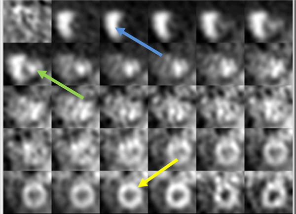
A mid-ventricular short-axis slice from a normal patient viewed over time following injection of the flow tracer. The upper left image is before activity reaches the heart and is essentially all noise. Proceeding left-to-right and down, the lower right image is the same mid-ventricular slice 5 minutes after injection. Note the activity first arrives into the right ventricle (blue arrow), then left ventricle (green arrow), then myocardial tissue (yellow arrow).

18 3-dimensional regions of interest (ROI) are generated [the standard 17 sement myocardial model and the LV blood compartment,⁴ based on the uptake later in the study (bottom row of Figure 1). The later images are summed to give a clearer image of the heart. The ROIs are then placed over each image volume in the time series to obtain the activity in each of the regions as a function of time (time activity curves (TACs).

Typical TACs for a clinical rest study are shown in Figure 2. Note that the activity first arrives in the LV (blood curve) and then the tissue. Once in the tissue, it is irreversibly bound and remains constant. Hence, the expected shape of the blood curve is a rapid rise to a peak as the bolus passes through the heart, and then a rapid fall to a low and constant value. The tissue curves start rising after the blood curve and reach a plateau value.

Figure 2.

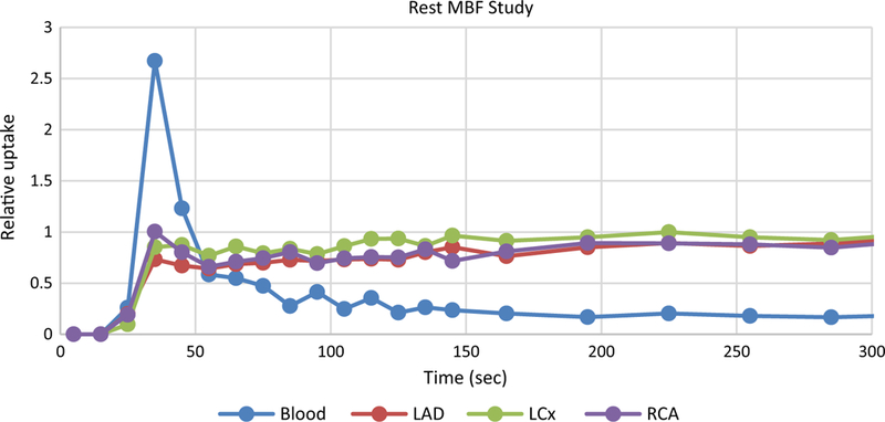
Typical rest uptake curves from a normal patient following infusion of the myocardial flow tracer.

The activity rapidly clears from the blood yet the measured blood curve in Figure 2 remains consistently above zero. This is entirely due to spillover from the surrounding tissue. The combined effects of the beating heart, respiratory motion, and finite resolution of the scanner all lead to tissue activity ‘spilling over’ into the blood measurement. Hence, a spillover correction must be performed to have accurate TACs. The finite resolution of the scanner also leads to the tissue activity being underestimated. To correct for this loss of activity, a ‘recovery coefficient’ is applied to the curves. A sign that these effects have been accurately corrected is the modeled blood curve approaching zero and staying flat after the bolus passes through the heart. This is discussed further below.

QUALITY CONTROL ISSUES

Figure 2 shows an example of well measured TACs from a typical normal patient. Unfortunately, the TACs often don’t have this ideal shape. Figure 3 shows patient curves where the initial data were not collected because the scanner was started after the bolus passed through the heart. A complete and reliable input function is required to calculate MBF so absolute flow cannot be determined for this study.

Figure 3.

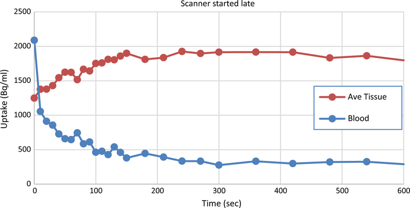
Example of data from a clinical study where the scanner was started late. The bolus has already passed through the left ventricle making an accurate determination of the input function impossible. MBF cannot be calculated in this case.

Figure 4 shows TACs from a clinical study that has 2 quality control (QC) issues. The erratic behavior of the TACs at the beginning of the acquisition is typical of detection systems when the number of events per second occurring in a detector exceeds its maximum count rate. The situation is termed ‘saturation’ and the output is usually either very high or very small numbers, sometimes switching between the two extremes. The scanner used to generate the data in this figure was saturated for about 50 seconds after the start of acquisition rendering this portion of the data meaningless. As the count rate decreased (as activity passed through the field of view), the detectors recovered. By about 100 seconds into this study, the detectors are recording events accurately. However, at 280 seconds, there is a spike in the blood curve and a matching dip in the tissue curve. This is caused by patient motion. In this case, the patient moved and then returned to the same place. If the curves were step-like, they would indicate that the patient moved to a new location and remained there.

Figure 4.

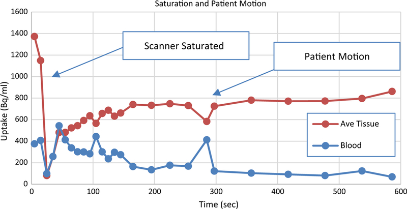
TACs from a clinical study that includes examples of a saturated scanner and patient motion. Erratic swings in the time activity curve, often from the maximum to 0 (or near zero) are signs of saturated detectors. The abrupt change at 280 seconds in the otherwise normal looking curves is a sign that the patient moved.

‘Upward creep’ was originally used to describe the upward movement of the heart seen in SPECT studies as the patient recovers from exhaustive physical exercise.⁵ In contrast, we observed movement of the heart in other directions as well. To encompass this possibility, we propose the term ‘myocardial creep’ to refer to the heart drifting within the thoracic cavity during the study (as opposed to complete patient motion and not to be confused with the beating motion of the heart). While its causes could be many, it is far more common during pharmacological stress so we posit one cause to be: diaphragmatic / breathing changes that occur as a side- effect of pharmacological vasodilation. Because of myocardial creep, even images from a completely compliant patient can exhibit signs of motion.

As described above, regions of interest are drawn on the later frames of the dynamic image set because it contains the clearest (least noise) image of the heart. The regions are then copied to all earlier frames to generate the TACs. If myocardial creep is present, the ROIs copied to the earlier frames will not be correctly positioned over myocardial tissue. If the heart is gradually creeping throughout the study (the usual case), then the earlier the frame the further off will be the positioning of the ROIs. Since the heart is the brightest object in the image (after the bolus has passed through the heart), a mispositioned region can only result in an underestimation of the activity in the myocardial tissue. And, the greater the mispositioning of the ROI, the more background will be included in the ROI and therefore, the greater is the underestimation of tissue activity. Because of this, myocardial creep results in the false appearance of rising tissue curves. When this is seen, most likely the last tissue activity in the TAC is correct while the earlier values are underestimated. An example is shown in Figure 5.

Figure 5.

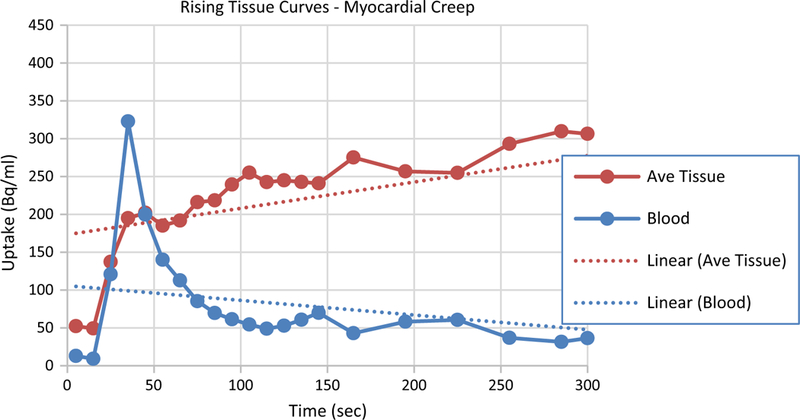
TACs from a clinical stress study that exhibits the characteristics of cardiac creep. Rising tissue curves after the tracer clears from the blood deviate from the expected curve shape (flat). Typically, this is caused by myocardial creep that is induced by the pharmacologic stressing agent.

QUALITY CONTROL

Quality control checks that should be performed on the TACs before calculating MBF.

Check	Description
Frame durations	Check that the scanner has accurately recorded scan start times and frame durations (which are critical for the modeling)
Saturation	Check count behavior for signs of saturation as bolus first passes through heart
Blood peak presence	Check for clear blood peak. If missing, the scanner was probably started too late after the injection
Blood peak width	A blood peak width of 20–70 seconds is expected. If the width is outside this range, the injection was infiltrated or there were other problems with the injection
Tissue curve tails	The tails of the tissue curves should be flat since the tracer is irreversibly trapped and the activity rapidly clears from the blood. Rising tissue curves are typical of gradual patient or cardiac drifting
Blood curve tail	The tail of the blood curve should be low and flat following similar reasoning from the tissue curves
Tissue curve discontinuities	Discontinuities (steps, peaks, or dips) are signs of likely patient motion
Modeled blood	The modeled blood curve should be flat and near zero after the bolus passes through the heart. If otherwise, it is a sign of improper spillover correction, or uncorrected cardiac movement during the study

IMPLICATIONS OF QUALITY ISSUES

Spillover and partial volume correcting the TACs from Figure 2 produces the curves shown in Figure 6. Note several things about this corrected curve relative to Figure 2: (1) the peak of the blood curve is slightly higher (blood recovery coefficient), (2) the tail of the blood curve approaches zero (spillover from tissue removed), (3) the tissue curves rise more gradually (blood spillover is removed), and (4) the tissue curves rise to a slightly higher value (tissue recovery coefficient). From TACs that represent an accurate representation of the true activity in the blood and tissue, flow can be estimated as the final tissue activity, which may be calculated as the mean of the frames after the activity becomes constant, divided by the area of the blood curve as demonstrated in Figure 6. For comparison, the full model derived flow for the average tissue in this study is 0.86 ml/min/g.

Figure 6.

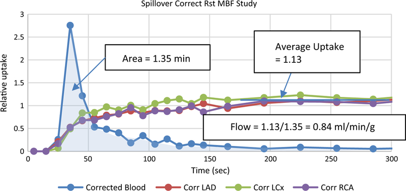
Spillover and partial volume corrected curves from Figure 2. An initial estimate of flow can be derived as the average uptake divided by the area of the input curve, as illustrated.

The effects of the quality issues discussed above can be understood by keeping Figure 6 in mind. If the estimated area of the blood curve is too high, then the calculated flow will be too low. If the measured activity in the tissue is an underestimate, then the calculated flow will be too low, and so on. A saturated scanner or late start to the scan prevents being able to determine the area of the blood curve, so it is not possible to calculate flow.

An understanding of how flow is calculated will help to know when a quality control issue can and cannot be overlooked. Movement of the type displayed in Figure 4 will probably have minimal effect on the calculated flow. The area of the blood curve wouldn’t be affected much by a later spike in the curves. And, the final average value of the tissue uptake also won’t be affected much. On the other hand, a gradual drifting of the heart as seen in Figure 5 will likely alter the flow calculation significantly. The average tissue uptake is not reliably determined. The spillover correction for the blood will be in error since it depends on an accurate estimation of the tissue activity, which is not the case here. Hence, the area of the blood curve will likely be in error. If the average tissue uptake and area of the blood curve have large errors, then the calculated flow will have a large error. It is important to note that the inaccurate flow value could be either too high or too low.

CONCLUSION

Absolute myocardial blood flow can give valuable information when forming a diagnosis for a particular patient. When high quality data are collected from a compliant patient (Figures 2 and 6), flow can be estimated with high precision. However, dynamic imaging and compartment modeling is more complicated than static imaging. There is a greater risk of artifactual results contaminating the final result. Because of this, it is critical that enhanced quality control is included with every flow calculation.

Abbreviations

MBF

Myocardial blood flow

BGO

Bismuth germanate

LSO

Lutetium oxyorthosilicate

LYSO

Lutetium-yttrium oxyorthosilicate

GSO

Gadolinium oxyorthosilicate

ROI

Region of interest

TAC(s)

Time activity curve(s)

QC

Quality control

References

- 1.Schindler TH, Schelbert H. Cardiac PET imaging for the detection and monitoring of coronary artery disease and microvascular health. JACC Cardiovasc Imaging. 2010;3(6):623–40. [DOI] [PubMed] [Google Scholar]
- 2.Maddahi J, Packard RR. Cardiac PET perfusion tracers: Current status and future directions. Semin Nucl Med. 2014;44(5):333–43. [DOI] [PMC free article] [PubMed] [Google Scholar]
- 3.Moody JB, Lee BC. Precision and accuracy of clinical quantification of myocardial blood flow by dynamic PET: A technical perspective. J Nucl Cardiol. 2015;22(5):935–51. [DOI] [PubMed] [Google Scholar]
- 4.Cerqueira MD, Weissman NJ. Standardized myocardial segmentation and nomenclature for tomographic imaging of the heart. A statement for healthcare professionals from the Cardiac Imaging Committee of the Council on Clinical Cardiology of the American Heart Association. Circulation. 2002;105(4):539–42. [DOI] [PubMed] [Google Scholar]
- 5.Friedman J, Van Train K. Upward creep of the heart: A frequent source of false-positive reversible defects during thallium-201 stress-redistribution SPECT. J Nucl Med. 1989;30(10):18–22. [PubMed] [Google Scholar]