Quantitative assessment of field strength, total intracranial volume, sex, and age effects on the goodness of harmonization for volumetric analysis on the ADNI database

Abstract

When analyzing large multicenter databases, the effects of multiple confounding covariates increase the variability in the data and may reduce the ability to detect changes due to the actual effect of interest, for example, changes due to disease. Efficient ways to evaluate the effect of covariates toward the data harmonization are therefore important. In this article, we showcase techniques to assess the “goodness of harmonization” of covariates. We analyze 7,656 MR images in the multisite, multiscanner Alzheimer's Disease Neuroimaging Initiative (ADNI) database. We present a comparison of three methods for estimating total intracranial volume to assess their robustness and correct the brain structure volumes using the residual method and the proportional (normalization by division) method. We then evaluated the distribution of brain structure volumes over the entire ADNI database before and after accounting for multiple covariates such as total intracranial volume, scanner field strength, sex, and age using two techniques: (a) Zscapes, a panoramic visualization technique to analyze the entire database and (b) empirical cumulative distributions functions. The results from this study highlight the importance of assessing the goodness of data harmonization as a necessary preprocessing step when pooling large data set with multiple covariates, prior to further statistical data analysis.

1. INTRODUCTION

Data harmonization is an important step for data mining and statistical analysis for many fields of research, especially in the era of big data (Agarwal, Shroff, & Malhotra, 2013). Such “goodness of harmonization” is important to ensure the optimal power of statistical analysis, because the effect of additional covariates introduces undesirable variations that may swamp the true effect of interest. In the field of neuroimaging, brain imaging databases such as the Alzheimer Disease Neuroimaging Initiative (ADNI) now include thousands of brain images (Mueller et al., 2005a) from multiple sites. In such databases, confounding covariates can enter at multiple steps due to differences in protocols for data acquisition (Jovicich et al., 2009), processing (Wyman et al., 2013), and analysis (Fortin et al., 2018; Fortin, Sweeney, Muschelli, Crainiceanu, & Shinohara, 2016; Frisoni & Jack, 2015; Yu et al., 2018).

Significant efforts are being directed to harmonize the data acquisition and processing protocols to minimize site‐related variations. The EADC‐ADNI harmonization protocol initiated by Frisoni and Jack (2015) aims to generate consensus for manual hippocampus segmentation among research groups around the world and to reduce the systematic bias of the data due to intrarater variability. The ENIGMA consortium (Thompson et al., 2017) studied the genetic‐association to harmonize the diffusion tensor imaging (DTI) (Jahanshad et al., 2013; Kochunov et al., 2015). Potvin et al. have constructed normative data of structure volumes and cortical thicknesses from large number healthy controls subjects across different studies by taking into account the effect of age, sex, total intracranial volume (TIV), scanner manufacture, and magnetic field strength (Potvin, Dieumegarde, & Duchesne, 2017; Potvin, Mouiha, Dieumegarde, & Duchesne, 2016). Mirzaalian et al. have proposed a multi‐model registration‐based framework to harmonize the raw diffusion MRI signal in a model‐independent manner and reduced the analysis bias on data acquired from multiple sites (Mirzaalian et al., 2016; Mirzaalian et al., 2018). Fortin et al. have addressed the importance of controlling the nonbiological variance (the scanner‐specific effects), effectively harmonizing the signal intensity of T1W image (Fortin et al., 2016), the fractional anisotropy (FA), and mean diffusivity (MD) for DTI (Fortin et al., 2017), as well as the automatically estimated cortical thickness (Fortin et al., 2018) improving the statistical and classification power for data analysis. Using the same harmonization methods (ComBat), Yu et al. have successfully removed the site effects from multisite resting‐sate fMRI data (Yu et al., 2018). Data harmonization also helps to improve the performance for machine learning algorithms, as removing unwanted covariates from the data not only help to improve the training accuracy but also help to generalize the model and prevent overfitting due to learning of signatures from unrelated covariates. Rozycki et al. (2018) have shown that data pooled from multisite with intersite image harmonization improves both group‐level statistical analysis and multivariate classification power compared to single site analysis.

The harmonization of the data can be affected by various sources of covariates. For instance, MRI‐derived structural volumetric measures such as hippocampal atrophy (Macdonald et al., 2014) and ventricle expansion (Nestor et al., 2008; Ott et al., 2010; Weiner, 2008) are important quantitative imaging biomarkers of disease progression and these are influenced by head size (measured via TIV) (Barnes et al., 2010; Hansen, Brezova, Eikenes, Haberg, & Vangberg, 2015; Jenkins, Fox, Rossor, Harvey, & Rossor, 2014; Voevodskaya, 2014). The measurement of head size itself and brain structural volumes concurrently are influenced by scanner field strength (1.5 T vs. 3 T) (Chow et al., 2015a; Chu et al., 2016; Jovicich et al., 2009; Macdonald et al., 2014). Sex is also an important source of demographic‐related variation in TIV and volumes of brain structures (Gur et al., 1991; Perlaki et al., 2014; Ritchie et al., 2018). Another source of individual‐level variation is due to normal aging‐related changes (Scahill et al., 2003; Takao, Hayashi, & Ohtomo, 2012; Taki et al., 2013) that are introduced when analyzing databases including subjects over a range of ages. Signatures of subtle structural change due to disease in these neuroimaging measures may be masked by the gross variations due to head size, sex, or age across subjects (Aoyagi et al., 1990; Barnes et al., 2010; Gur et al., 1991; Ingalhalikar et al., 2014; O'Brien et al., 2011; Perlaki et al., 2014; Rathore, Habes, Iftikhar, Shacklett, & Davatzikos, 2017; Trune, Mitchell, & Phillips, 1988) or because of the selection of image processing pipelines (Nordenskjold et al., 2013). These sources of variation have become much more prominent as multisite databases are beginning to be pooled. Changes in data distribution and variability measures before and after adjusting for such covariates are therefore important indicators of how well multiple sources of data are harmonized. For example, when analyzing the brain structure volume, the difference between subgroups of each covariates (i.e., the male and female, 1.5 T and 3 T MRI scanner) should be minimized after the data harmonization.

In this article, we propose two qualitative and one quantitative method to assess such “goodness of harmonization”. One of the qualitative (visual) methods is a heatmap of normalized regional structural volumes. This panoramic visualization of the entire database, which we term as Zscapes, offers a visual assessment of the harmonization procedure. Harmonized measures can be visually assessed after removal of one or more covariates by viewing the data in its entirety and any systematic biases remaining can be seen in patterns of color changes across the database. Another visual technique we propose is through the use of empirical cumulative distribution functions (ECDFs) where the covariate‐induced variability introduces overlaps between the distributions of each measure. After harmonization, the ECDFs converge to a common distribution if the effect of interest (such as disease) is the primary source of remaining variability. We also propose the use of the Kolmogorov–Smirnov (K‐S) statistic as a quantitative measure of the overlap of each of the ECDFs, before, and after accounting for covariates. Using these tools, we investigated the effect of TIV, field strength, sex, and age toward brain structure volumetric analysis. To the best of our knowledge, this is the first study to investigate multivariate multifeature effects toward demographic‐related data harmonization over a large number (7,656 images) taken from the ADNI database.

2. METHODS

In this study, we analyzed the Alzheimer's Disease Neuroimaging Initiative (ADNI) database. ADNI is a large cross‐sectional and longitudinal neuroimaging database with three clinically diagnosed groups at the time of the assessments: the cognitive normal (CN) group, the mild cognitive impairment (MCI) group, and the Alzheimer's disease (AD) group. The CN group is treated as the reference group for all analyses. In the following sections, we detail each of the steps of analysis. Briefly, we segmented the gray matter structures using FreeSurfer and extracted the raw volumes for each FreeSurfer‐labeled structure. We present three TIV measurement methods on these ADNI images and compare their robustness. We also compare the TIV estimation methods on paired 1.5 T/3 T scans. We performed a comparison of two methods for head size normalization using TIV, namely the proportional‐ and the residual‐based methods. We evaluated the effect of the covariates such as field strength, TIV, sex, and age on volumetric analysis. We then propose two qualitative (visual) and a quantitative method to assess the “goodness of harmonization” of data before and after accounting for the covariates.

2.1. Experimental data

2.1.1. The ADNI database

T1‐weighted structural MRI data along with corresponding demographic and scanner‐specific information were obtained from the publicly available ADNI database (http://adni.loni.usc.edu) (Jack et al., 2008; Mueller et al., 2005a; Mueller et al., 2005b; Weiner et al., 2013). A general description of the image acquisition parameter protocol for the data set is described in detail in a previous study by Chow et al. (2015b), and detailed scanner‐specific parameters are described by Jack et al. (2008). The MRI database we analyzed consists of a total of 7,656 scans collected from 1,727 subjects, acquired longitudinally for up to 13 timepoints (from baseline up to 120 months) for which covariate information on field strength, sex, age, and clinical diagnosis was available. The ADNI data set includes a mixture of 1.5 T and 3 T images, with subjects' average ages at 75 ranging from 55 to 95.

2.1.2. Database with pairs of 1.5 T/3 T scans for each subject

To study the effect of field strength on the TIV estimation (Section 3.5), we also analyzed MR images from 187 subjects (91 male and 96 female) with both 1.5 T and 3 T MRI scans (755 images for each field strength) taken back to back at multiple timepoints (up to 36 months). This set of 1,510 longitudinally scanned images was collected by the ADNI MRI core specifically for methods comparison (Wyman et al., 2013), and the corresponding 1.5 T scans have been included in the main ADNI data set described earlier. A subset of this data set has been used to show improved statistical power for 3 T over 1.5 T for measuring hippocampal volume (Chow et al., 2015b).

2.2. FreeSurfer structure segmentation and volume extraction

We used the volume‐based stream of the FreeSurfer processing pipeline version 5.3.0 (Desikan et al., 2006) to segment 87 anatomical structures (left/right separated) of the cortical (Fischl, 2004) and subcortical (Fischl et al., 2002) gray matter and extracted their volumes. The FreeSurfer processing pipeline consists of five steps: (a) affine registration to the MNI305 spaces, (b) B1 intensity inhomogeneities correction, (c) nonrigid registration to the MNI305 spaces, and (4) atlas‐based structure labeling based on the maximum likelihood of the probability atlas. The FreeSurfer volume‐based pipeline is described in the papers by Fischl et al. (2004 , 2002). All images were preprocessed with nonparametric nonuniform normalization (N3) (Sled, Zijdenbos, & Evans, 1998) prior to the structure segmentation and TIV estimation.

2.3. Evaluation of the automatic TIV estimation methods

The brain structure volumes are known to be dependent on the individual's head size (Barnes et al., 2010; Hansen et al., 2015; Jenkins et al., 2014; Voevodskaya, 2014). The TIV is a measurement of head size and is a crucial covariate to be adjusted for when performing volumetric analysis (Hansen et al., 2015; Wolf et al., 2003). Accurate estimation of the TIV is therefore important to minimize the bias during data analysis (Sargolzaei et al., 2014). Ideally, TIV measurement is performed by segmenting the cranial vault directly and measuring its volume, but other indirect ways of estimating the TIV without segmenting the cranial vault have also been proposed. We compared three different automatic TIV estimation methods. Among them, FreeSurfer and SPM are two widely used brain image processing and analyzing packages that provide fully automated process to estimate the TIV indirectly through affine scaling and tissue segmentation (Hansen et al., 2015; Heinen et al., 2016; Keihaninejad et al., 2010; Malone et al., 2015; Nordenskjold et al., 2013; Pengas, Pereira, Williams, & Nestor, 2009; Sargolzaei et al., 2015a; Vagberg, Ambarki, Lindqvist, Birgander, & Svenningsson, 2016). In addition, the multi‐atlas label fusion (MALF)‐based TIV estimation has been proposed, which segments the cranial vault directly and demonstrated higher correlation and similarity measurements when compared with the manual segmentation as ground truth (Huo, Asman, Plassard, & Landman, 2017; Manjon et al., 2014; Schaerer et al., 2012).

For large databases like ADNI, it is very difficult to undertake manual segmentation for TIV to perform the standard analysis based on Dice overlap accuracy. Therefore, we adopt two alternative evaluation criteria to study the robustness of automated estimation: the longitudinal consistency and test–retest reliability.

First, the adult bony cranial vault is not expected to change over time (Whitwell, Crum, Watt, & Fox, 2001), and previous studies on elderly subjects (age > 52) demonstrated no association between the measured TIV and aging for both healthy and AD patients (Edland et al., 2002; Jenkins et al., 2014). The ADNI data set includes elderly adults subjects (age range between 55 and 95 years old) and hence their TIV is not expected to change during the ADNI study. Therefore, we chose to use longitudinal consistency defined as the change of estimated TIV over time as a metric to evaluate the robustness of the automated estimation methods. Longitudinal consistency of TIV is thus used as an outcome metric to identify the TIV estimation method delivering the most consistent measures over time.

Second, we evaluate the robustness of the three TIV estimation methods by analyzing the test–retest reliability using a subset of cross‐sectional “open access series of imaging studies” (OASIS‐1) with consecutive scans dedicated for evaluating the robustness of the image processing methods. The pairwise percentage volume difference between the test and retest data were used as an outcome metric for assessing the robustness of the TIV estimation methods (Bland & Altman, 1994; Giavarina, 2015; Myles & Cui, 2007).

2.3.1. Three TIV estimation methods

FreeSurfer

TIV is estimated using a scaling factor derived from an affine transformation between the template and the target and applying that scaling factor to the TIV of the template (Buckner et al., 2004).

SPM

The most recent version of SPM (Malone et al., 2015) utilizes a generative model to integrate partial‐volume tissue classification with image registration and intensity nonuniformity correction (Friston, & Ashburner, 2005). Each brain image is segmented into white matter (WM), gray matter (GM), cerebral spinal fluid (CSF), and additional three tissue types (bone, soft tissue, and air/background) for more accurate characterization of tissue composition in the image. We used the “Tissue Volumes” utility introduced in SPM12 which wrapped and constrained the tissue segmentation within a manually corrected TIV mask, then summed up the WM, GM, and CSF volumes to obtain the estimated TIV (Malone et al., 2015).

Multi‐atlas label fusion

We used the OASIS‐BC2 atlas by Huo et al. (2017) containing 27 T1 MR images taken from the OASIS data set (Marcus et al., 2007; Marcus, Fotenos, Csernansky, Morris, & Buckner, 2010) as the templates in image registration‐based label propagation and fusion. The corresponding manual TIV labels were created based on the corresponding CT images of the same subjects to ensure very accurate segmentation following the BrainCOLOR protocol (Klein & Tourville, 2012), which is also part of the brain structure atlas provided by the MICCAI12 Multi‐Atlas Grand Challenge (Landman & Warfield, 2012). The image intensity for each template‐test image pair is normalized, the template MRI is registered to the target MR using first an affine and then a nonrigid large deformation diffeomorphic metric mapping (LDDMM) algorithm (Beg, Miller, Trouve, & Younes, 2005). Each manually segmented template TIV Label was then propagated from the template atlas to the target image with the derived deformation map and finally fused together to generate the TIV mask with weighted majority voting. All TIV segmentations were visually inspected by two experienced raters for quality control.

2.3.2. Robustness analysis

We evaluate the robustness of automated estimation through two criteria: the longitudinal consistency and test–retest reliability. To evaluate the longitudinal consistency, we use linear mixed‐effect (LME) model with random‐intercept (Equation (1)) (Bernal‐Rusiel, Greve, Reuter, Fischl, & Sabuncu, 2013; Xu, Shen, & Pan, 2014) to measure the correlation between TIV and age. For this experiment, TIV is considered as the dependent variable, whereas age is the independent variable (predictor) with fixed effects, with the field strength (1.5 T and 3 T) and sex (male and female) modeled as the independent variables with random effect, each with two levels. We use the restricted maximum likelihood approach (REML) to fit the model:

$$\mathrm{TI}{\mathrm{V}}_{\mathrm{i}}={\mathrm{\beta }}_0+{\mathrm{\beta }}_1{\mathrm{X}}_{\mathrm{i}}+\sum _{\mathrm{r}=1}^{\mathrm{R}}{\mathrm{z}}_{\mathrm{i},\mathrm{r}}{\mathrm{b}}_{\mathrm{m}\left(\mathrm{r},\mathrm{i}\right)}^{\mathrm{r}}+{\mathrm{\epsilon }}_{\mathrm{i}}$$ (1)

where β ₁ is the fixed effect coefficient for the age variable (X _i) for the ith subject, and $b_{m\left(r,i\right)}^r$ is the random effect vector for the rth grouping variable (b ¹: field strength, b ²: sex) and level m(r,i) (m ⊂ (0,1)).

To evaluate the test–retest reliability, we analyzed a data set from the OASIS‐1 database (Marcus et al., 2007) dedicated for testing the reproducibility of image processing methods. This data set includes 20 healthy subjects between 20 and 34 years of age who underwent two consecutive MRI scans using the same 1.5 T scanner. Detailed scanning protocol and subject demographics of the OASIS‐1 reliability data set are described in Marcus et al. (2007). Bland–Altman analysis is used to study the pairwise percentage volume difference (PVD, Equation (2)) between the estimated TIV from the test data and the retest data for assessing the robustness of the three methods (Bland & Altman, 1994; Giavarina, 2015; Myles & Cui, 2007).

$$\mathrm{PVD}=\frac{\mathrm{TI}{\mathrm{V}}_{\text{test}}-\mathrm{TI}{\mathrm{V}}_{\text{retest}}}{\left(\mathrm{TI}{\mathrm{V}}_{\text{test}}+\mathrm{TI}{\mathrm{V}}_{\text{retest}}\right)/2}\times 100\%$$ (2)

where TIV_test is the TIV estimated from the test data, and TIV_retest is the TIV estimated from the retest data.

2.4. Evaluation of the TIV normalization methods

There are two methods commonly used for TIV normalization (Sanfilipo, Benedict, Zivadinov, & Bakshi, 2004): (a) the proportion method (Jernigan, Zatz, Moses, & Berger, 1982), and (b) the residual method (O'Brien et al., 2011; Sanfilipo et al., 2004). The proportion methods simply divide the structure volume by the TIV; while the residual method (Equation (3)) models the structural volume as a linear combination of the TIV and the residual terms, computes the linear regression from the reference (CN) group measures, and takes the residual ε _i (the difference between the actual measure and that predicted from using the reference‐group fitted linear model) as the normalized measure for further analysis.

$${\mathrm{V}}_{\mathrm{i}}={\mathrm{\beta }}_0+{\mathrm{\beta }}_1\mathrm{TI}{\mathrm{V}}_{\mathrm{i}}+{\mathrm{\epsilon }}_{\mathrm{i}}$$ (3)

Specifically, it has been recommended to use the standardized residual, also known as the W‐score (defined as W _i = (ε _i − μ _εCN)/σ _εCN), rather than the raw residual when accessing the structural changes such as atrophy (Collij et al., 2016; La Joie et al., 2012; O'brien & Dyck, 1995). The W‐score is the Z‐score of the residuals where μ _εCN is the mean of the residuals within the reference group (CN) group and σ _εCN is the standard deviation (SD).

2.5. TIV variation due to scanner field strength difference

To study the influence of scanning field strength (1.5 T vs. 3 T) on TIV, we performed an additional analysis using a second ADNI cohort of subjects with both 1.5 T and 3 T MRI scans back to back at multiple timepoints (up to 36 months) as described in Section 3.1.2. We measured the correlation between the field strength (1.5 T and 3 T) and the TIV for each processing method, and calculated the coefficient of determination R ². In addition, we utilize Bland–Altman analysis (Equation (3)) to study the pairwise PVD similar to the test–retest analysis in the section 2.4. Here, the TIV_test is the 1.5 T TIV, and the TIV_retest is the 3 T TIV. We also calculated the empirical cumulative density function (ECDF) for each field strength for male and female subjects separately.

2.6. GLM‐based combined accounting of covariates

We evaluate the data distribution and variability of the structural volume before and after harmonization (adjusting for the covariates such as field strength, TIV, sex, and age). We used the general linear model (GLM), where the structure volume and all the other covariates are independent (predictive) variables (Equation (4)).

$${\mathrm{V}}_{\mathrm{i}}={\mathrm{\beta }}_0+\sum _{\mathrm{r}=1}^{\mathrm{R}}{\mathrm{\beta }}_{\mathrm{r}}{\mathrm{X}}_{\mathrm{r},\mathrm{i}}+{\mathrm{\epsilon }}_{\mathrm{i}}$$ (4)

where X _i are covariates such as field strength, TIV, sex, and age of each subject i, and R is the total number of independent variables. We can analyze the variability in data that is explained by these covariates individually and together. In this article, we selected and presented some covariate combinations to illustrate the difference in terms of data harmonization in different scenario: (a) the scanner specific covariate (field strength) only; (b) the individual‐specific covariate (TIV) only; (c) the combination of field strength and TIV; and (d) the combination of field strength, TIV, and demographic covariate (sex and age).

2.7. Evaluation of “goodness of harmonization” of a database

The goal of harmonization of covariates is to remove the unwanted sources of variation (field strength, TIV, sex, and age) within acquired measures (structural volumes) and retain only those sources of variation that are of interest (such as disease). The hypothesis is that variation of structural volume measures within each diagnostic group (CN, MCI, and AD) will be progressively diminished as more unwanted covariates are removed and minimized when all covariates have been suitably accounted. As a result, the distance between distributions of measures across the effect of interest (e.g., disease diagnostic groups CN, MCI, and AD) will be progressively enhanced and maximized when all unwanted covariates have been accounted for and removed. These outcome metrics form the basis of the following methods proposed to demonstrate the “goodness of harmonization”.

2.7.1. Visualization of “goodness of harmonization” using Zscapes

To evaluate the variation of the structure volume feature across the entire sampled population after each covariate regression, we first assess the within‐group variation by calculating the Z‐score of each measure X _i for subject i given by $Z_i=\left(X_i-{\mu }_{X_{\mathit{CN}}}\right)/{\sigma }_{\mathit{CN}}$ where ${\mu }_{X_{\mathit{CN}}}$ is the mean value of the reference (CN) group, and σ _CN is the SD of the reference (CN) group. In the cases where residual method is used to regress out covariates, Z‐scores effectively become the W‐scores. The Z‐score represents the distance of each measurement to the reference group mean, normalized by the reference group SD. By measuring the Z‐score, changes in each structure with respect to the reference mean are highlighted and comparable across range of structural volumes due to standardization as a multiple of the SD.

We plot the Z‐score over the entire ADNI database analyzed such that all structure volumes for a subject are presented in one column, and each FreeSurfer‐derived structure volume is presented in one row across all subjects. This resulting panoramic heat map is denoted as a Zscape and enables the assessment of patterns across all the subjects and all the structures at the same time.

2.7.2. Visualization of “goodness of harmonization” using ECDF

To quantitatively evaluate and compare the data variability before and after the harmonization, we plotted data distribution for each structure's volume using the ECDF and tested the goodness‐of‐fit. As the MCI group is heterogeneous, that is, it includes subjects who will develop AD (progressive MCI) and subjects who will not develop AD in their lifetime (stable MCI), we exclude the MCI group in this step and only include the CN and AD group, to control the effect of unknown covariates when evaluating the goodness of harmonization. We first calculated the ECDF for the CN and AD group, different sex group (male and female), and field strength group (1.5 T and 3 T) separately. As the covariates of TIV, sex, and field strength are removed, first individually, then in combination, we expect the disease remains the primary source of variability ultimately and hence the ECDFs for the residual of each measure are expected to coalesce to a common ECDF for the control and AD group, respectively.

2.7.3. Measurement of “goodness of harmonization” using the K‐Sstatistic

We propose to use the K‐S test, a nonparametric test for the “goodness‐of‐fit” of the ECDF, which is widely used to evaluate the maximum absolute difference between the CDFs of sample distributions (Arnold & Emerson, 2011). We used the two‐sample K‐S test ((Massey, 1951), Equation (5)) to measure the separation of the sample distributions and quantitatively compare the ECDFs for sex, age, and diagnosis. The hypothesis is that, for more harmonized data, the distance between the ECDF curves of the subgroups with different value of confounding covariates (e.g., field strength and sex) will be smaller, and the distance among the ECDF curves of different diagnostic groups should be larger.

$$D_{m,n}=\underset{\text{sup}}{x}\left( |F_{1,m}\left(x\right)-F_{2,n}\left(x\right)| \right)$$ (5)

where F _1,m(x) and F _2,n(x) are the ECDF of the two samples. In the K‐S test, the two distribution are considered as significantly different (reject the null hypothesis) when the score is above the D_m,n.

$$D_{m,n}>\sqrt{-\frac{1}{2}\ln \frac{\alpha }{2}}\sqrt{\frac{m+n}{\mathit{mn}}}$$ (6)

in which α is the reject level and is set to 0.05, and we denote the level of rejection as $D_{m,n}^{*}$.

We selected the hippocampus to demonstrate the effect of different regression results to separate the ECDF of different subgroups for each grouping variables, given that hippocampal atrophy is considered one of the signature hallmarks for AD progression. We included all the subjects currently available in ADNI who are diagnosed as either CN or AD to evaluate the result of the comparison and compared the difference between the two diagnostic groups (CN vs. AD), as well as the two sex groups (male vs. female), and the two field strength groups (1.5 T vs. 3 T).

3. RESULTS

3.1. Demographic analysis

The results of demographic analysis are listed in Table 1. Statistical comparisons of the age distribution were performed at each level of the categorization, that is, among diagnostic groups, between male and female within each diagnostic group, and between 1.5 T and 3 T within each sex subgroup. The population age in the MCI groups is found to be significantly smaller than the other two groups (CN and AD). Significant age differences were detected for all the comparisons between male and female groups and between the 1.5 T and 3 T groups. These point to the necessity of adjusting for age when performing groupwise structure volume comparison, as age affects regional brain structure volumes (Li et al., 2013).

Table 1.

Demographic analysis of the entire ADNI database. Some subjects were scanned on 1.5 T scanner at early timepoints and 3 T scanner for their later timepoints

Diagnosis (age, mean ± SD years)	Sex (age)	Field strength (age)	Scans	Subjects
CN (76.15 ± 6.24)	Femalea (75.79 ± 6.11)	1.5 Ta (78.13 ± 5.09)	509	169
		3 T (73.30 ± 6.13)	706	132
	Male (76.50 ± 6.34)	1.5 Ta (77.49 ± 5.87)	575	198
		3 T (75.12 ± 6.71)	611	114
MCI* (74.64 ± 7.70)	Femalea (73.44 ± 8.04)	1.5 Ta (75.18 ± 7.78)	1,008	294
		3 T (72.12 ± 7.99)	1,115	284
	Male (75.41 ± 7.37)	1.5 Ta (77.11 ± 7.04)	784	239
		3 T (73.54 ± 7.28)	591	163
AD (76.06 ± 7.47)	Femalea (75.15 ± 7.93)	1.5 Ta (75.99 ± 7.55)	333	150
		3 T (73.29 ± 8.42)	667	221
	Male (76.75 ± 7.04)	1.5 Ta (77.07 ± 6.88)	236	113
		3 T (76.10 ± 7.31)	521	170

Note. CN = cognitively normal, MCI = mild cognitive impairment, AD = clinically diagnosed Alzheimer's disease. The mean ± SD of age distribution for each group is shown in the brackets (unit: Year). Statistical comparison of the age distribution was performed at each level of the categorization. One‐way ANOVA was performed among CN/MCI/AD group. Unpaired two‐tailed t‐test were performed between male and female population for each diagnostic group, as well as between 1.5 T and 3 T for each sex subgroup within each diagnostic group. Multiple comparisons were corrected with false discovery rate (FDR) set to 0.05.

^aThe population age in the MCI group is statistically significantly smaller than the CN and AD groups. Significant age differences were found in all subgroup comparisons.

3.2. TIV estimation

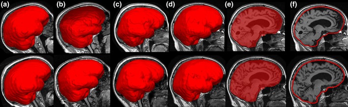
Figure 1 shows the sample sagittal images of MALF TIV overlaid on the brain image for male and female subjects, acquired at both 1.5 T and 3 T MRI. All 7,657 images passed the visual inspected quality check. The MALF not only provides an estimate for TIV but also provides a delineation of the boundary of the cranial vault giving a three‐dimensional (3D) mask of the cranial‐vault independent of the brain tissue outline. The surface and shape information of TIV mask, in addition to the volume measure, could also be potentially useful for additional analyses. Comparatively, the FreeSurfer TIV only estimates the intracranial volume through affine‐based scaling factor; therefore, no FreeSurfer TIV mask is available. In SPM, a TIV mask is generated in the subject space during the pipeline process (through the template‐based nonrigid registered “reverse brain mask” as part of the “new segmentation” method in SPM 12). However, in SPM 12, this TIV mask is not used to calculate the final measurement of TIV but rather used to constrain the final TIV calculation through the summation of threshold tissue probability map. Compared to this single template‐based TIV mask, the MALF provides a 3D TIV mask through the fusion of multiple nonrigid registered template masks (Huo et al., 2017) giving a direct measure of the 3D surface/shape of the cranial vault.

Figure 1.

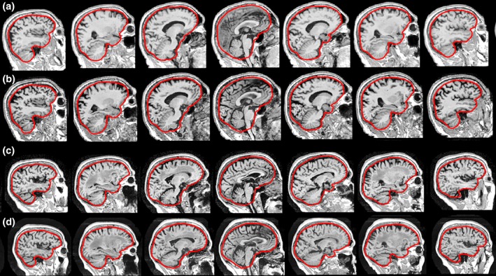
Sagittal view of multiple atlas label fusion (MALF) estimated TIV overlaid on the brain images for (a) 1.5 T image of a male subject; (b) 3 T image for the same male subject; (c) 1.5 T image of a female subject; (d) 3 T image of the same female subject. This visualization shows the MALF method is able to generate accurate outlines of the cranial vault based on the OASISBC2 atlas, and the cranial vault contour shapes are comparable for the same subject on both field strengths [Color figure can be viewed at http://wileyonlinelibrary.com]

3.2.1. Longitudinal consistency

Figure 2a–c shows the longitudinal trajectory of TIV normalized to the baseline volume across all available time‐points using the FreeSurfer, SPM, and MALF methods. The estimate of TIV exhibits variability as a function of different acquisition timepoints (in months). FreeSurfer TIV estimate on 1.5 T data (top row) shows a small negative longitudinal trend. SPM TIV shows better overall longitudinal consistency, although there are more variations in the data (more data points lie outside the ±5% change from the baseline). The MALF exhibits the most visually consistent longitudinal TIV among the three methods, and most of the estimated TIV measures are within the ±5% variation range

Figure 2.

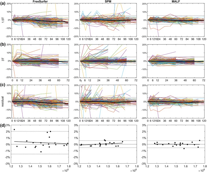
(a–c) Longitudinal trajectories of percentage change of TIV from baseline for both 1.5 T (top row) and 3 T (bottom row) over time (in months). Each colored line represents the longitudinal trajectory of an individual subject. Median of TIV trajectory is shown in the black line. The dashed line represents the ±5% variation range. The MALF method shows smaller longitudinal variations of TIV as compared to FreeSurfer and SPM methods. (d) Visualization of the test–retest reliability analysis via the Bland–Altman plot. Dashed lines represent 95% confidence interval (CI) of the mean difference, and solid lines represent the linear regression result that fit the data. The FreeSurfer (left column) showed larger CI than the SPM (middle column) and MALF (right column) [Color figure can be viewed at http://wileyonlinelibrary.com]

To quantitatively evaluate the longitudinal consistency, we used LME model to remove the effects of field strength and sex on the linear intercept (base TIV) and examine the relationship between TIV estimates and scanning time (Lee, Nakamura, Narayanan, Brown, & Arnold, 2018). The results of LME model are shown in Table 2. Theoretically, there should be no association between the adult TIV and time. No significant correlation between age and TIV was detected with all three methods, with FreeSurfer exhibits the largest coefficient (−0.45%/year) and largest variance (−0.34%/year), SPM showed a modest coefficient (−0.15%/year) and variance (0.25%/year) and MALF showed the smallest correlation (0.11%/year) and variance (0.11%/year). In addition, Figure 2c shows the TIV residual after fit with the LME Model. Most the MALF‐estimated TIV lies within the ±5% residual range, while for both FreeSurfer and SPM, there are large proportion of residuals that exceed the ±5 range. In summary, all three TIV estimation methods showed good longitudinal consistency, with MALF demonstrating marginally better performance.

Table 2.

Quantitative evaluation of the longitudinal consistency and test–retest reliability for three TIV estimation methods (FreeSurfer, SPM, and MALF) across all the time points of 1.5 T and 3 T

	LMEM coefficient versus time			Bland–Altman analysis
	Estimated coefficient (%)	Residual variance (%)	p‐value	95% confidence interval (%)
FreeSurfer	−0.45	0.34	.73	−1.5 to 2.0
SPM	−0.15	0.25	.83	−0.52 to 0.58
MALF	0.11	0.11	.31	−0.55 to 0.55

Note. The estimated coefficient of age (first column) represents the longitudinal slope of TIV change across time. The residual variance (second column) represents the SE after fitting LME model. The p‐value (third column) reflects the significance to detect the correlation between the coefficient (age) and the dependent variable (TIV). The forth column reports the 95% confidence interval of the Bland–Altman analysis, which shows the percentage difference between the estimated TIV of the test and retest data. All three methods showed p‐values larger than 0.1, and the estimated coefficients are with the same magnitude of the residual variance, which indicates no significant correlation between age and TIV were detected. MALF showed the smallest coefficient and SE among the three methods, although all three methods show comparable level of consistency. The MALF methods also showed the smallest and most balanced confidence interval among all the three methods.

3.2.2. Test–retest reliability

Figure 2d and Table 2 showed the result of test–retest reliability using Bland–Altman analysis. The FreeSurfer showed largest confidence interval (CI) (−1.53 to 2.01%) of the mean difference among the three, followed by SPM (−0.52 to 0.58%) and MALF (−0.55% to 0.55%).

In conclusion, MALF showed the most robust performance over FreeSurfer and SPM both in terms of longitudinal consistency and test–retest reliability. Since MALF also provides an accurate 3D mask of the intracranial space; therefore, we used the MALF‐based estimate of TIV in the following analyses.

3.3. TIV variation due to scanner field strength difference

When comparing TIV estimated from 1.5 T and 3 T images using the second cohort, which includes back to back scanned images of both 1.5 T and 3 T, both the correlation (Figure 3a–c) and PVD (Figure 3d,f, Bland–Altman plots) (Giavarina, 2015) showed good agreement. However, as seen in these results, the TIV estimates for 3 T images are smaller than the 1.5 T estimates across all three methods (FreeSurfer, SPM, and MALF). Such field strength‐related discrepancy is also shown in the plot of ECDF (Figure 3g–i) of the 1.5 T and 3 T TIV, where the ECDF of 3 T TIVs are shifted leftward (representing relatively lower value) compared with the 1.5 T TIVs.

Figure 3.

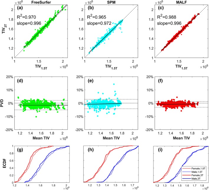
Comparing TIV at 1.5 T and 3 T for all three methods: FreeSurfer, SPM, and MALF. (a–c) Correlation, (d–f) agreement in terms of percentage volume difference (PVD) using bland–Altman plots and (g–i) empirical cumulative distribution function (CDF). The PVD in the bland–Altman plot is defined in equation (2). (a–c) All three methods show good correlation, with MALF being the highest. TIV at 3 T is slightly lower than at 1.5 T. (d–f) Visualization of agreement between the values via the Bland–Altman plot shows qualitatively lower disagreement between 1.5 T and 3 T TIVs with MALF as evidenced by a narrower 95% confidence interval (CI) (dashed lines) as compared to FreeSurfer and SPM. Furthermore, no systematic biases toward larger or smaller TIVs are noted for each method. (g–i): The 3 T TIV values are slightly lower than 1.5 T values and the female TIV values at each field strength are markedly lower than male TIV values (x axis unit: mm³) [Color figure can be viewed at http://wileyonlinelibrary.com]

3.4. Correlation between ROI volume and TIV

Figure 4 shows the correlation between volumes of a set of FreeSurfer‐derived ROIs (14 subcortical/cortical structures and lateral ventricle) and the TIV for the CN group across all timepoints. The 1.5 T and 3 T data are shown separately. An overall positive correlation between ROI volumes and TIV is found, indicating that larger head sizes generally translate to larger brain structures. However, the strength of the correlation appeared to vary among different structures. The variation of the correlation indicates that different structures in the brain are scaled with TIV in a nonproportional way.

Figure 4.

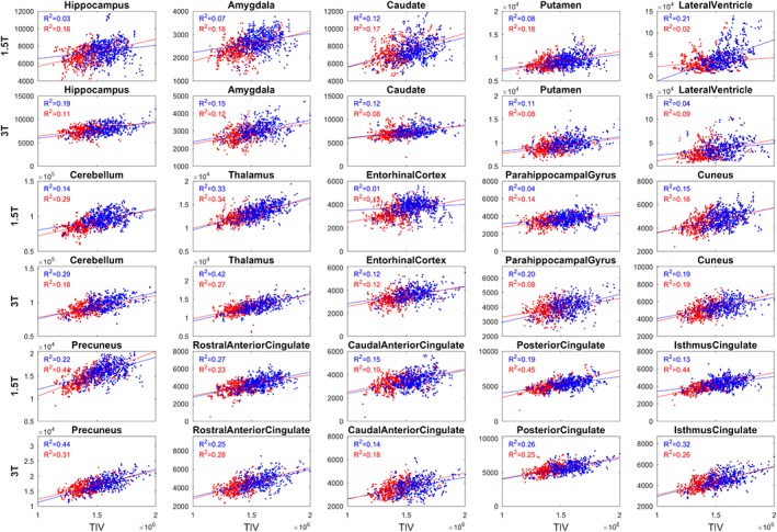
Correlation between the MALF‐based TIV (x axis) and some selected structure volumes (y axis) for the CN group for males (blue) and females (red). The correlations are shown with the left and right sides volumes combined, and separated for field‐strength (1.5 T separate row as 3 T). the TIV of male subjects tends toward larger values at both field strengths compared to TIV of females. Males with larger TIV showed larger structure volumes compared to female subjects as evidenced by a positive correlation between the ROI volumes and TIV. The strength of correlation varies across ROIs [Color figure can be viewed at http://wileyonlinelibrary.com]

3.5. Evaluation of “goodness of harmonization”

In this section, we evaluated the distribution and variation of the brain structure volumes over the entire ADNI database before and after accounting for covariates such as TIV, scanner field strength, sex, and age using (a) Zscapes and (b) ECDFs.

3.5.1. Visualization of the goodness of harmonization using volume Zscapes

Figure 5 shows the Zscape—a panoramic view of the Z‐score of each gray matter ROI volume for all subjects in the ADNI database (with CN group regarded as the reference group). The CN, MCI, and AD diagnostic groups are shown separately, each divided into male and female, which are further divided into 1.5 T and 3 T. Within each Zscape plot, the horizontal axis is sorted according to age at the time of scan in ascending order. Color spectrum from blue to red represent the value of the Z‐score ranging from −6 to +6, showing the level of volume shift from the mean of the reference (CN) group. If the data are fully harmonized, we expect the visual patterns within any diagnostic group (CN/MCI/AD) to be homogeneously distributed with minimum intragroup variation, which means minimum male‐v‐female or 3 T‐v‐1.5 T differences, and minimum volume variation due to normal aging. Figure 5 demonstrates different levels of data harmonization after adjusting for the different confounding covariates.

• Figure 5a: No covariates adjusted. There is a clear distinction between each covariate subgroup: the structure volume decreases (left to right) with age given trend toward cooler colors. The volumes in male group appear larger (warmer colors) than the female group (cooler colors). The structure volumes at 3 T appear larger (warmer colors) than at 1.5 T (cooler colors). Compared to Figure 3, which showed smaller 3 T TIV compared to 1.5 T, the result shows that the effect of field strength toward the TIV is not proportionally scaled across different tissue types. Figure 8 in the later section shows more in‐depth investigation of this finding

• Figure 5b: Adjusting for field strength. The discrimination between 1.5 T and 3 T has been controlled for, whereas the distinction between male and female and across age is still visible

• Figure 5c: Volume normalized by direct division with TIV. Contrary to the raw data Zscape in (a), the normalized female structural volumes tend toward larger values (warmer colors) than the normalized male volumes. The variation between 1.5 T and 3 T colors still persist after the TIV normalization

• Figure 5d: Volume normalization by TIV with the residual method. Compared to (c), the regression normalized male and female volume W‐scores tend to become more similar, although the differences between 1.5 T and 3 T volumes still remain

• Figure 5e: Adjust field strength then divide by TIV. Compared to (b), which only adjusts for field strength, little improvement of harmonization is observed

• Figure 5f: Adjust field strength and TIV with the residual method. Compared to (b), which only adjust for field strength, the difference between male and female group is reduced significantly as well, indicate a strong correlation between the TIV and sex. This finding aligns with the results shown in Figures 3g–i and 4

• Figure 5g: Adjust field strength, TIV, and sex. Compared to (f), the improvement of data harmonization in terms of reducing the female/male structure volume difference is not obvious, as most of the difference has been removed when the TIV is adjusted

• Figure 5h: Adjust all covariates, including field strength, TIV, sex, and age. This harmonization process has removed the color patterns across the subgroups leading to a uniform pattern of structure volume distribution across subjects within each disease diagnostic group

Figure 5.

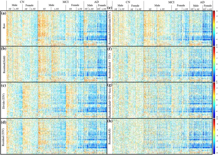
The Zscape of all FreeSurfer segmented GM structure across the entire ADNI, showing the Z‐score of all the structures for every subject in the database. Data are first categorized into three diagnostic groups: CN, MCI, and AD, with CN group be the reference control group to calculate the Z‐score. Each diagnostic group is then further divided into female and male groups, which are then further separated into the 3 T and 1.5 T subgroups. Within each 1.5 T and 3 T subgroup, the data were sorted left to right according to increasing age. Only Z‐score beyond ±1 SD of the CN group is shown. Color spectrum from blue to red represent the value of the Z‐score ranging from −6 to +6, showing the level of volume shift from the mean of the reference (CN) group. (a) The raw structure volume showed systematic volume difference between the 1.5 T and 3 T subgroup, as well as between the male and female group. Within each subgroup, the volume is also decreased when the age increases (from left to right) reflecting the effect or normal aging. (b) Regress out only the covariate of field strength remove the systematic difference between 1.5 T and 3 T. (c) Normalize the TIV with proportional method (direct divide the volume with TIV) does no't remove intradiagnosis‐group variation. (d) Regress out the TIV only reduces the sex‐based data variation, but the systematic bias between 1.5 T and 3 T remains. (e) Regress out the covariate of field strength followed by proportional based TIV normalization doesn't reduce the data variation further. (f) Regress out both the field strength and the TIV removes the systematic volume difference between the 1.5 T and 3 T as well as between the male and female, which is similar to (g) regress out the TIV, field strength and female, indicating that TIV and sex is highly correlated. (h) Including age in the model further remove the effect of structure volume reduction due to normal aging. In summary, the residual‐based covariate regression reduces the variation within each individual diagnostic group [Color figure can be viewed at http://wileyonlinelibrary.com]

Figure 8.

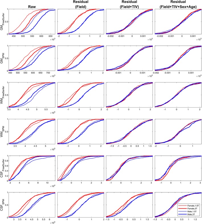
ECDF of tissue volume (GM/WM/CSF) from FreeSurfer and SPM taken from the CN group only. Thick line = 3 T, thin line = 1.5 T; red = female, blue = male. Field strength corrected residual shows a prominent sex‐effect, whereas correcting additionally for TIV accounts for the variability attributed to sex as well. In addition, the ECDFs show that GM is scaled larger at 3 T field strength (thicker lines of the 3 T ECDF to the right of thinner lines for the 1.5 T ECDF, for both males and females), while WM and CSF are scaled smaller at the 3 T field strength (thicker lines to the left of thinner lines) indicating nonlinear scaling of different tissue types across field strengths [Color figure can be viewed at http://wileyonlinelibrary.com]

3.5.2. Visualization of “goodness of harmonization” using ECDF

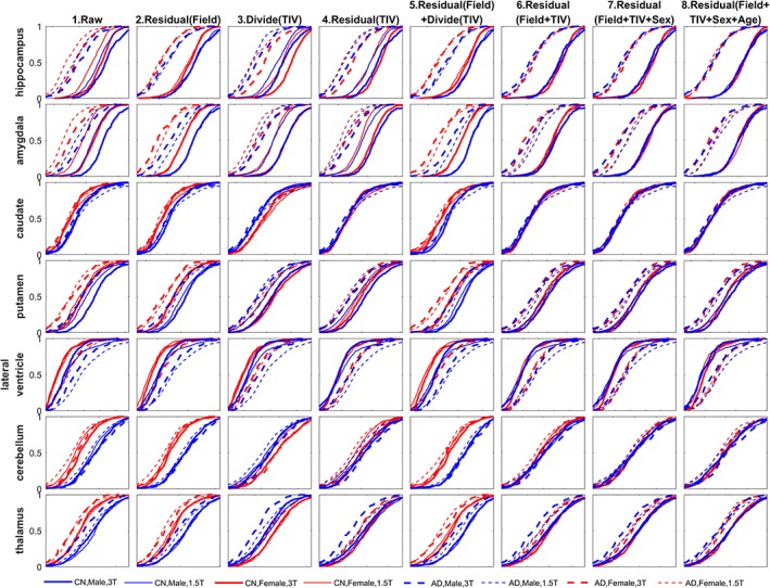
Figures 6 and 7 show the ECDF for a selected sampling of subcortical and cortical structures, respectively, including both the left and right hemisphere's structural volume measures to simplify the presentation. The ECDFs of the raw measures (column 1) show marked scatter and reduced separations between CN and AD groups prior to the control of covariates. The female (red) ECDF curves are generally to the left as compared to the male (blue) ECDF curves indicating overall smaller uncorrected regional volumes in females. The 1.5 T measures (thin lines) are generally to the left of the 3 T measures (thick lines) indicating that gray matter volumes are lower at 1.5 T relative to 3 T except for the lateral ventricles where the pattern is reversed indicating that ventricles are larger on 1.5 T. The AD group measures (dashed lines) are generally to the left or coincident with the CN group measures (solid lines) indicating that structural volumes are lower, or preserved, in AD as compared to controls, except for the ventricles where the pattern is reversed, indicating enlargement of ventricles in AD.

Figure 6.

The empirical cumulative distribution function (ECDF) of the volumetric measures taken from a select few subcortical structures. Solid line = CN, dashed line = AD; thick line = 3 T, thin line = 1.5 T; red = female, blue = male. The residual in the title represents the standardized residual after regression (W‐score with respect to the CN reference group). Note the overlap of ECDFs in the raw measures. As the variability attributed to field strength, TIV, sex, and age are accounted for traversing from left to right, the ECDFs of the harmonized measures tend to coalesce leaving ECDFs for the CN and AD distribution [Color figure can be viewed at http://wileyonlinelibrary.com]

Figure 7.

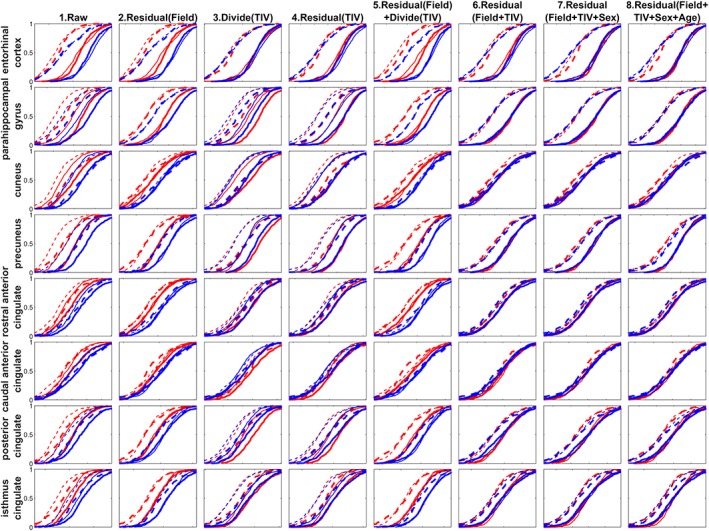
The empirical cumulative distribution function (ECDF) of the volumetric measures taken from a select few cortical structures. Solid line = CN, dashed line = AD; thick line = 3 T, thin line = 1.5 T; red = female, blue = male. The residual in the title represents the standardized residual after regression (W‐score with respect to the CN reference group). Note the overlap of ECDFs in the raw measures. As the variability attributed to field strength, TIV, sex, and age are accounted for traversing from left to right, the ECDFs of the harmonized measures tend to coalesce leaving ECDFs for the CN and AD distribution [Color figure can be viewed at http://wileyonlinelibrary.com]

After accounting for field strength (second column), the systematic bias between 1.5 T and 3 T measures is reduced as shown by the coalescing of the corresponding 3 T (thick) and 1.5 T (thin) ECDF lines. The variabilities due to female/male differences still remain, as evidenced by the leftward shift of the female ECDFs (red lines) compared to the male ECDFs (blue lines). Removing TIV (by division as in third column or by regression as in fourth column) without adjusting for field strength shows that the male and female ECDFs tend to coalesce, as TIV is correlated to sex, but the variation due to field strength is evident in the separation of the 1.5 T (thin) and the 3 T (thick) ECDF lines.

Using a GLM with field strength and TIV further (column 6) reduces the systematic bias between female and male ECDFs, which is similar to the ECDF after introducing the sex covariate to the GLM (seventh column), reaffirming the correlation between TIV and sex. Interestingly, controlling for field strength with regression residual, and then dividing by TIV, as is often done in literature, does not as satisfactorily account for these covariates as shown in column 5 compared to column 6 as the distributions generally do not coalesce. Introducing age into the GLM (eighth column) does not show a marked change in the ECDFs, indicating no distinctive effect of age towards the distribution pattern when comparing among the different covariate subgroups (i.e., the age‐dependent volume variation is similar for each subgroup).

The ECDFs also showcase the influence of AD on these structures relative to the CN group by the leftward separation of the ECDFs after accounting for covariates. The hippocampus and amygdala (in Figure 6), and entorhinal cortex, para‐hippocampal gyrus, precuneus, posterior and isthmus cingulate (in Figure 7) show lowering of volume in the AD group as the dashed lines all coalesce into a single distribution leftward of the coalesced solid lines. Ventricles, on the other hand, show enlargement, as expected (in Figure 6). On the other hand, for putamen, thalamus, the dashed lines (AD) and solid lines (CN) are relatively closer compared to other subcortical structures (in Figure 6), indicating a smaller effect of AD to lower the volume. Interestingly, for entorhinal cortex (Figure 7, first row), normalizing the volume by dividing with TIV (column 3) or residual with TIV (column 4) already accounted for the variability induced by other covariates. This indicates that different structures have different nonlinear relationships to field strength and TIV, and visual evaluation of “goodness of harmonization” of measures can help assess whether the accounting for covariates via the chosen method achieved the intended result.

We further plot the ECDF of gray matter (GM), white matter (WM), and cerebrospinal fluid (CSF) tissue volume of the CN group extracted from both the FreeSurfer and SPM pipelines (Figure 8) to assess the normalization effectiveness on the total GM/WM/CSF compartments. The field‐strength corrected residuals in this Figure show a prominent sex‐effect, whereas correcting additionally for TIV accounts for the variability attributed to sex as well. In addition, the ECDFs of the raw tissue volume (first column) show that GM is scaled larger at 3 T field‐strength (thicker lines of the 3 T ECDF to the right of thinner lines for the 1.5 T ECDF, for both males and females), whereas WM and CSF are scaled smaller at the 3 T field‐strength (thicker lines to the left of thinner lines) indicating nonlinear scaling of different tissue types across field strengths.

3.5.3. Quantitative evaluation of data harmonization based on ECDF

To quantitatively assess the shift of ECDFs after accounting for each covariate, we performed the K‐S test between two subgroups for each of the three variables (diagnosis, field strength, and sex) for hippocampus (both left and right), a region considered to be a hallmark of AD‐induced degeneration. Figure 9a shows the CDF comparing four different normalizations, and Figure 9b–d shows the result of K‐S test representing the statistical distances between the distributions. In Figure 9b–d, the y axis shows the value of K‐S statistic D _m,n, and the dashed line represents the threshold value $D_{m,n}^{*}$ to reject the null hypothesis that the two sample distributions come from the same population. We anticipate that the D _m,n statistic will be maximized between subgroups of CN and AD, the main effect of interest (e.g., CN 1.5 T female vs. AD 1.5 T female will show larger separation after normalization) and minimized between nuisance covariates that need to be reduced/removed such as 1.5 T vs. 3 T (e.g., 1.5 T CN male vs. 3 T CN male ECDFs will show reduced separation after normalization). When comparing the diagnostic group (panel b), all normalization methods showed significant differences between CN and AD. The value of K‐S statistic D _m,n increases after including all covariates in the GLM, representing a larger difference between sample ECDFs, effectively increasing the power for discrimination (red bar, representing the fourth column, “Residual (field+TIV_sex_age)” in panel a). When comparing 1.5 T and 3 T (panel c), the significant difference between the two distributions is removed after all covariates have been controlled. The difference between the ECDF of male and female groups (panel d) becomes insignificant after controlling the TIV as the standardized residual of the GLM, confirming the strong correlation between the TIV and subject sex.

Figure 9.

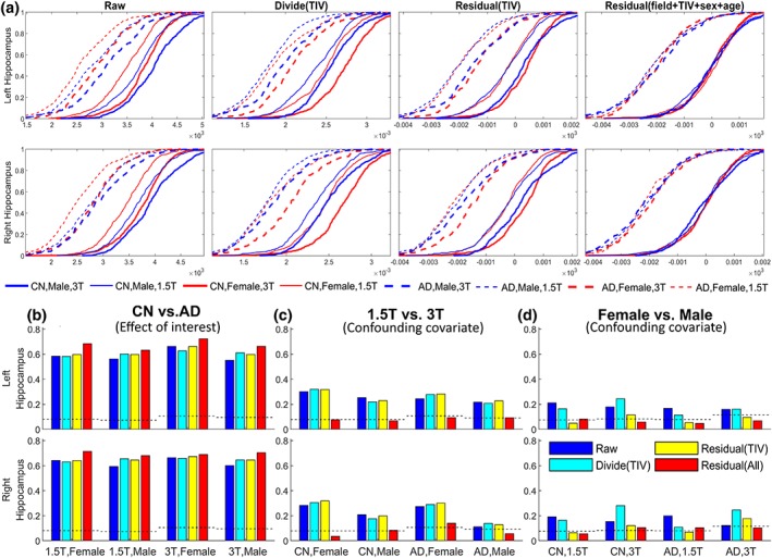
Panel (a): Comparison of normalization methods for hippocampus volumes as a function of field strength and TIV, sex, age. ECDFs for structural volumes of each subgroup are shown after accounting for covariates. The rightmost column, for example, shows the residual after regression for TIV, age, sex and field strength showing that the ECDFs of all subgroups coalesce closer into ECDFs of CN and AD (the effect of interest). Solid line = CN, dashed line = AD; thick line = 3 T, thin line = 1.5 T; red = female, blue = male. Panel (b–d): The Kolmogorov–Smirnov (KS) statistic (equation (5)) comparing the ECDF separation within each subgroup. In each panel, different colors represent different normalization methods used in panel (a). Panel (b) shows the K‐S statistic between the ECDFs of CN and AD groups. For example, the group of 4 bars on the left in panel b are the K‐S statistic between the ECDFs of CN 1.5 T female and AD 1.5 T female subgroups (the thin red lines in panel (a), both solid and dashed lines) for each of the four normalization methods (corresponding to the four columns in panel [a]). the K‐S statistic is the highest for the “residual (field+TIV+sex+age)” method (red) indicating an increasing separation between the ECDFs with this method of harmonization. Panel (c) shows the K‐S statistic between 1.5 T and 3 T group ECDFs. As an example, the bars on the left in this panel show K‐S statistic for 1.5 T CN female and 3 T CN female for each of the four methods. The separation between these ECDFs decreases after “residual (field+TIV+sex+age)” method (red) is utilized. Panel (d) shows the K‐S statistic between female and male groups. As an example, the bars on the left in this panel show K‐S statistic between the female 1.5 T CN ECDF and the male 1.5 T CN ECDF for the four methods. This panel shows that the separation between female and male ECDFs is reduced with the “residual (TIV)” (yellow) and “residual (field+TIV+sex+age)” (red) method [Color figure can be viewed at http://wileyonlinelibrary.com]

4. DISCUSSION

4.1. “Goodness of harmonization”

In the quest toward improved understanding of brain structure and function, recent neuroimaging databases such as ADNI leverage data sharing from multiple sites, and multiple research laboratories to increase the number of imaging scans available for analyses. Differences in site‐specific parameters (such as acquisition pulse sequences) or processing‐specific parameters (such as segmentation protocols) can introduce undesirable variability in data that can reduce the power to detect smaller effect sizes of interest. To reduce/remove such unrelated and undesirable sources of variability, a significant amount of recent collaborative research effort has been directed toward harmonization of acquisition and processing protocols. Techniques for assessment of “goodness of harmonization” are relevant even with harmonized data acquisition and processing protocols, as systematic sources of variability can still exist due to unaccounted methodological or demographic covariates potentially biasing all downstream analyses (Shinohara et al., 2017).

In this study, we presented several methods to assess the “goodness of harmonization” of images with varying field strength (1.5 T/3 T), TIV (proportional/residual normalization), sex (male/female), and age as covariates. Using these methods, we demonstrate the effect of different data harmonization choices, before, and after controlling for the effect of these covariates. Our experiments indicate that the GLM‐based residuals are the appropriate choice for these covariates for volumetric analysis purposes. Group difference analysis can of‐course directly incorporate multiple covariates into the GLM (Lenoski, Baxter, Karam, Maisog, & Debbins, 2008). By directly analyzing the residuals at each stage of the GLM correction, deeper insights assessing the accounting of covariates can be obtained. These harmonized residuals are inputs for the development of and/or testing of classification models. Proper modeling and accounting of covariates that help reduce spurious variability while retaining the variability of interest in the input features for classification are known to help increase the discrimination between the patterns related to the effect of interest inherent in these features (Rozycki et al., 2018).

We used the K‐S statistic (Massey, 1951) to quantify the distance between ECDFs after covariate normalization. We note that this quantification can also be performed with other alternative distance measures and statistical tests such as Discrete Cramer‐von Mises (CVM) criterion (Anderson, 1962), Kullback–Leibler divergence (Kullback, 1997), or the k‐sample Anderson‐Darling test (Scholz & Stephens, 1987) depending on the distribution of the data. In addition, although the covariates we evaluated in this study only include scanner field strength, TIV, sex and age, the proposed methods can be extended to evaluate the effect of additional covariates including but not limited to technique covariates such as scanner vendor (Lee et al., 2018) or demographic/biological covariates such as disease risk‐related genes, such as Apolipoprotein E (APOE) mutation status. In addition, further research is needed to identify universal thresholds for assessing “good” or “bad” harmonization, which may likely depend on the databases being pooled, and the particular covariates chosen for the study.

Fortin et al. have previously reviewed and compared several different data harmonization methods (Fortin et al., 2017), such as functional normalization (Fortin et al., 2014), RAVEL (Fortin et al., 2016), surrogate variable analysis (SVA) (Leek & Storey, 2007), ComBat (Johnson, Li, & Rabinovic, 2007), and RUV (Gagnon‐Bartsch & Speed, 2012). The tools developed in this study for assessing “goodness of harmonization” could be potentially used for comparison of these competing harmonization strategies. In addition, although we only evaluated the goodness of harmonization for data within a single database (ADNI) in this study, the data harmonization can also be extended to pool data from multiple studies by including additional site‐specific covariates (Fortin et al., 2018).

4.2. TIV estimation and normalization

TIV is an important covariate for neuroanatomical studies looking at the changes in brain structure. However, accurate TIV estimation from T1‐weighted (T1W) brain MRI is not easy given the lack of adequate contrast between the skull and the CSF. Currently, the best validated and widely used TIV estimation methods are found in FreeSurfer (Buckner et al., 2004) and SPM toolboxes (Keihaninejad et al., 2010), and the MALF method (Huo et al., 2017; Schaerer et al., 2012). FreeSurfer (version 5.3.0) uses a template with precalculated TIV, which is affinely registered to the target image, and uses the scaling factors derived from the affine matrix to approximate the TIV (Buckner et al., 2004). In SPM, the TIV is calculated as the sum of the all intracranial tissues, with additional tissue class most introduced in the recent version of SPM 12 (e.g., external CSF as appose to part of the entire CSF classes in the early version) and regularized through wrapping the tissue segmentation with a manually corrected TIV mask (Keihaninejad et al., 2010) to improve the segmentation accuracy. The more rigorous definition of T1‐based TIV in SPM appears to be more consistent compared to FreeSurfer's scaling‐based estimation (Hansen et al., 2015; Keihaninejad et al., 2010; Sargolzaei et al., 2014; Sargolzaei et al., 2015a; Sargolzaei et al., 2015b), and is less affected by the brain atrophy (Pengas et al., 2009). However, both the FreeSurfer and the SPM8 automatic TIV estimation introduce systematic overestimation (Nordenskjold et al., 2013), which has been alleviated in SPM12 in which case a new method is introduced using template registration, which improves accuracy (Malone et al., 2015) and consistency (Heinen et al., 2016) of both TIV estimation, as well as brain volume measurements (Heinen et al., 2016; Vagberg et al., 2016).

Conversely, the MALF approach has demonstrated great accuracy in brain structure segmentation and parcellation, brain extraction (Heckemann et al., 2015), and skull stripping (Roy, Butman, & Pham, 2017). Schaerer et al. (2012) used a MALF framework (STAPLE) to estimate the TIV on ADNI data set and demonstrated better performance compared to FreeSurfer and SPM. Manjön et al. introduced a TIV extraction framework (Manjön et al., 2014) using a MALF‐based TIV as an extension of the brain extraction framework BEaST by including extra‐CSF in the manual atlas templates to obtain the entire TIV using conditional mask dilation (only over CSF voxels) followed by manual correction. More recently, Huo et al. (2017) applied an improved MALF framework (non‐local Spatial STAPLE‐NLSS) and reported better TIV estimation accuracy compared to SPM12 and FreeSurfer, validated using a semimanual segmented atlas of CT‐MRI image pairs as gold standard true TIV volume.

As the aim of the longitudinal consistency analysis is to evaluate the performance of the automated procedure from the three commonly used image processing packages (FreeSurfer, SPM, and MALF) with minimal or no human intervention to ensure the unbiased validation and comparison, we show all the TIVs estimated from all the subjects from these three methods. Those samples whose percentage change lies outside the ±5% variation range (Figure 2) are particularly highlighted to enhance the visual comparison across the three methods.

4.3. 3D TIV mask versus a scalar for volume

One advantage of MALF over other TIV methods such as FreeSurfer and SPM is the readily available 3D mask of the intracranial vault (a sample shown in Figure 10). SPM also generated a TIV mask in the subject space during the pipeline process (through the single template‐based nonrigid registered “reverse brain mask” as part of the “new segmentation” method in SPM 12). However, this TIV mask is not used to calculate the final measurement of TIV but rather to constrain the final TIV calculation through the summation of threshold tissue probability map. Compared to this single template‐based TIV mask, the MALF provides a 3D TIV mask through the fusion of multiple nonrigid registered template masks resulting in higher accuracy (Huo et al., 2017). While studying the shape of subcortical structures, such as the hippocampus, a typical approach is to perform affine registration of the segmented hippocampus ROI to a template hippocampus segmentation prior to nonrigid registration‐based shape analysis (Wang et al., 2007). However, not only may head size influences the size of brain structures, the shape of the cranial vault could also potentially influence the shape of brain structures in a nonisotropic manner. If this is the case, the shape of the intracranial vault could be used to perform nonisotropic normalization of the shape of brain structures such as the hippocampus to account for this 3D covariate of cranial‐vault shape. Normalization of cranial vault shape could, therefore, be important for studying shape changes of brain structures and is an interesting topic for future investigation.

Figure 10.

The sagittal view of sample images showing the overlay of the surface rendering of the 3D TIV mask estimated using the MALF with the corresponding T1 brain MR. Top row: 1.5 T, bottom row: 3 T (a) sample male CN subject, (b) sample female CN subject, (c) sample male AD subject, and (d) sample female AD subject. (e,f) The TIV mask of the same subject in (d) with an overlaid view (e) and contour view (f) [Color figure can be viewed at http://wileyonlinelibrary.com]

4.4. TIV normalization methods

The two commonly used methods proposed to account for the influence of TIV variations when analyzing changes in brain structure volumes are the proportional and the residual methods (O'brien et al., 2006; O'Brien et al., 2011; Voevodskaya, 2014). Sanfilipo et al. (2004) have performed a theoretical comparison between the proportional and residual methods for TIV normalization. The results of that study showed that the proportional method may aggregate errors that come from the numerator (structure volume) and the denominator (TIV), which can be observed from Figure 5c,e. On the other hand, the residual method guarantees that the error is minimized in the predicted value through the least square solution of the linear regression. The flexibility of residual methods also enables the TIV to be combined with other covariates for better intragroup harmonization (Figure 5d,f,h). One limitation of the residual method is the requirement of large enough sample in the reference group to derive linear coefficient to fit the TIV (the covariate) and structure volume (the dependent variable), unless such coefficient is generated a priori. However, this is not an issue when performing analyses on large databases such as ADNI.

4.5. Influence of covariates on TIV and brain tissue volumes

Our results show that, as is previously known, male TIV are generally larger than female TIV for both field strengths 1.5 T and 3 T (Figures 3g–i and 4). Larger TIV could lead to an assumption of a tendency toward larger brain structure volumes (a uniform scaling effect for all structures). Indeed, positive correlation between TIV and ROI volume is observed as shown in Figure 4. However, the strength of correlation varies across structures indicating that not all structures are uniformly larger with larger TIVs. This suggests that structural volumes in the brain are nonuniformly scaling with head size as measured by TIV.

TIV is found smaller on 3 T than at 1.5 T for both male and female subjects (Figure 3). Jovicich et al. have previously reported systematic smaller TIV from 1.5 T than the 3 T counterpart using FreeSurfer with 25 subjects (Jovicich et al., 2009). Keihaninejad et al. have proposed an SPM5‐based TIV estimation method—reverse brain mask (RBM), and reported over‐estimation of TIV from 1.5 T an under‐estimation the 3 T data when compared with manually defined ground truth with smaller samples (five healthy and two AD subjects [Keihaninejad et al., 2010]). Heckemann et al. (2011) studied a large number of subjects (n = 176) from ADNI with a semi‐automatic method (Freeborough, Fox, & Kitney, 1997; Zhang, Brady, & Smith, 2001) and also showed smaller 3 T TIV than 1.5 T. A recent study by Heinen et al. compared the TIV of 10 subjects and reported smaller 3 T TIV compared to 1.5 T using FreeSurfer 5.3.0, while interestingly no such significance TIV differences was reported with SPM12 (Heinen et al., 2016) in which the author attribute to the potentially explanation due to the improved estimation accuracy with the newer version of the analysis package. However, our result showed that the SPM 12 also showed significant smaller 3 T TIV compared to 1.5 T data, also the difference is smaller than FreeSurfer. The difference in the results of the two study may be due to the much increased sample size of the data set used in this study (n = 187) compared to the study of Heinen et al. (n = 10) which significantly increases the effect size.

There is currently no consensus yet to the explain field strength‐dependent TIV difference. Chu et al. reported similar finding that the brain volume measured from the 3 T data is smaller than the 1.5 T data and concluded that this is due to the lower image contrast presented in the 1.5 T data, which causes the over‐segmentation of the brain volume at the boundary between the parenchyma and CSF compartments because of the effect of partial volume averaging (Chu et al., 2016). In another words, the improved tissue contrast in the 3 T data may be helping to prevent over‐segmentation.

Possible biases of MRI‐derived volume measurements could also come from other scanner‐specific factors such as the effect of field strength different on the B1 intensity inhomogeneities correction (Jovicich et al., 2009). The ADNI MR imaging core used standardized preprocessing protocol to remove the intensity inhomogeneity in the data (Jovicich et al., 2006; Mueller et al., 2005b), although further studies are required to investigate the effect of field strength toward the preprocessing steps.

Lateral ventricles are smaller on 3 T than at 1.5 T (Figure 4), for both male and female subjects. This trend is seemingly more prominent for males than for females as evidenced by slightly larger separation for male ECDFs for lateral ventricle volumes. The fact that gray matter is larger at 3 T versus 1.5 T for both males and females, whereas white matter and CSF are smaller at 3 T (Figure 8) further indicating a nonuniform scaling of tissue compartments with scanner field strength. A previous study by Brunton et al. has also reported the similar observations using SPM8 and concluded that the CSF/WM/GM tissue volume measurement from 1.5 T and 3 T is not directly comparable in voxel‐wise analysis with tools such as SPM (Brunton et al., 2014). These tissue type‐dependent volume variations might further affect the TIV estimation, especially by the SPM method which estimates the TIV through a combination of CSF/WM/GM volumes (Malone et al., 2015). The differential effect of field strength toward different tissues may be because of the physics‐based properties of MR‐induced tissue relaxation times.

Interestingly, the influence of other covariates (sex and field strength) is not uniformly distributed across tissue types and across gray matter structure. Comparison between Figure 5a,c indicates that the difference of gray matter structure volume between male and female is smaller than the difference in TIV, so the TIV difference between sex is also not simply proportionally scaled across tissue. In addition, Figure 8 shows that the effect of field strength (1.5 T vs. 3 T) is also nonuniform across tissue types.

Finally, due to differences in TIV definition, the TIV estimates differ among the three methods, with SPM estimates being the smallest TIV and FreeSurfer the largest. Similar differences have been reported by previous studies (Freeborough et al., 1997; Heckemann et al., 2011; Heinen et al., 2016; Jovicich et al., 2009; Keihaninejad et al., 2010; Zhang et al., 2001).

4.6. Limitation of the current study

Reuter et al. have introduced the longitudinal stream in the FreeSurfer framework (Reuter & Fischl, 2011; Reuter, Rosas, & Fischl, 2010; Reuter, Schmansky, Rosas, & Fischl, 2012). Xu et al. (2014) have recommended initializing the segmentation of within‐subject longitudinal images with an average template for each subject and within subject registration across longitudinal data. This is a valid procedure for analyses such as longitudinal hippocampus volume change. On the other hand, the affine scale‐based TIV estimation in the FreeSurfer may have limited benefit from the use of this longitudinal stream; hence, in this article, we have used the standard FreeSurfer cross‐sectional stream to estimate TIV and segmentation for each image without taking advantage of the potential availability of longitudinal context where available. The evaluation of FreeSurfer longitudinal stream toward TIV estimation is suggested for future analyses.

5. CONCLUSION

In conclusion, we have proposed two qualitative and one quantitative method to assess the “goodness of harmonization” of covariates such as field strength, TIV, sex, and age for volumetric analysis of brain MR imaging data. Our results show that normalization of covariates based on a GLM model can be adopted based on their satisfactory assessment at harmonizing the selected covariates. The methods proposed for assessing goodness of harmonization can be used for comparing existing and novel harmonization methods. With these tools, diverse databases can be harmonized and assessed for “goodness of harmonization” before further statistical analysis.

CONFLICT OF INTEREST

There is no conflict of interest to declare from all authors.

Ma D, Popuri K, Bhalla M, et al. Quantitative assessment of field strength, total intracranial volume, sex, and age effects on the goodness of harmonization for volumetric analysis on the ADNI database. Hum Brain Mapp. 2019;40:1507–1527. 10.1002/hbm.24463

REFERENCES

- Agarwal, P. , Shroff, G. , & Malhotra, P. (2013). Approximate incremental big‐data harmonization. In Proceedings of the 2013 I.E. International Congress on Big Data, BigData 2013, pp. 118–125.
- Anderson, T. W. (1962). On the distribution of the two‐sample Cramer‐von Mises criterion. The Annals of Mathematical Statistics, 33(3), 1148–1159. [Google Scholar]
- Aoyagi, M. , Kim, Y. , Yokoyama, J. , Kiren, T. , Suzuki, Y. , & Koike, Y. (1990). Head size as a basis of gender difference in the latency of the brainstem auditory‐evoked response. International Journal of Audiology, 29(2), 107–112. [DOI] [PubMed] [Google Scholar]
- Arnold, T. B. , & Emerson, J. W. (2011). Nonparametric goodness‐of‐fit tests for discrete null distributions. The R Journal, 3(2), 34–39. [Google Scholar]
- Barnes, J. , Ridgway, G. R. , Bartlett, J. , Henley, S. M. , Lehmann, M. , Hobbs, N. , … Fox, N. C. (2010). Head size, age and gender adjustment in MRI studies: A necessary nuisance? NeuroImage, 53(4), 1244–1255. [DOI] [PubMed] [Google Scholar]
- Beg, M. F. , Miller, M. I. , Trouve, A. , & Younes, L. (2005). Computing' large deformation metric mappings via geodesic flows of diffeomorphisms. International Journal of Computer Vision, 61(2), 139–157. [Google Scholar]
- Bernal‐Rusiel, J. L. , Greve, D. N. , Reuter, M. , Fischl, B. , & Sabuncu, M. R. (2013). Statistical analysis of longitudinal neuroimage data with linear mixed effects models. NeuroImage, 66, 249–260. [DOI] [PMC free article] [PubMed] [Google Scholar]
- Bland, J. M. , & Altman, D. G. (1994). Statistics notes: Correlation, regression, and repeated data. BMJ, 308(6933), 896. [DOI] [PMC free article] [PubMed] [Google Scholar]
- Brunton, S. , Gunasinghe, C. , Jones, N. , Kempton, M. , Westman, E. , & Simmons, A. (2014). A voxel‐wise morphometry comparison of the Adni 1.5T and Adni 3.0T volumetric Mri protocols. Alzheimer's & Dementia, 10(4), P823. [DOI] [PMC free article] [PubMed] [Google Scholar]
- Buckner, R. L. , Head, D. , Parker, J. , Fotenos, A. F. , Marcus, D. , Morris, J. C. , & Snyder, A. Z. (2004). A unified approach for morphometric and functional data analysis in young, old, and demented adults using automated atlas‐based head size normalization: Reliability and validation against manual measurement of total intracranial volume. NeuroImage, 23(2), 724–738. [DOI] [PubMed] [Google Scholar]
- Chow, N. , Hwang, K. , Hurtz, S. , Green, A. , Somme, J. , Thompson, P. , … Apostolova, L. (2015a). Comparing 3T and 1.5T MRI for mapping hippocampal atrophy in the Alzheimer's disease neuroimaging initiative. American Journal of Neuroradiology, 36(4), 653–660. [DOI] [PMC free article] [PubMed] [Google Scholar]
- Chow, N. , Hwang, K. S. , Hurtz, S. , Green, A. E. , Somme, J. H. , Thompson, P. M. , … Apostolova, L. G. (2015b). Comparing 3T and 1.5T MRI for mapping hippocampal atrophy in the Alzheimer's disease neuroimaging initiative. American Journal of Neuroradiology, 36(4), 653–660. [DOI] [PMC free article] [PubMed] [Google Scholar]
- Chu, R. , Tauhid, S. , Glanz, B. I. , Healy, B. C. , Kim, G. , Oommen, V. V. , … Bakshi, R. (2016). Whole brain volume measured from 1.5T versus 3T MRI in healthy subjects and patients with multiple sclerosis. Journal of Neuroimaging : Official Journal of the American Society of Neuroimaging, 26(1), 62–67. [DOI] [PMC free article] [PubMed] [Google Scholar]
- Collij, L. E. , Heeman, F. , Kuijer, J. P. A. , Ossenkoppele, R. , Benedictus, M. R. , Moller, C. , … Wink, A. M. (2016). Application of machine learning to arterial spin labeling in mild cognitive impairment and Alzheimer disease. Radiology, 281(3), 865–875. [DOI] [PubMed] [Google Scholar]
- Desikan, R. S. , Segonne, F. , Fischl, B. , Quinn, B. T. , Dickerson, B. C. , Blacker, D. , … Killiany, R. J. (2006). An automated labeling system for subdividing the human cerebral cortex on MRI scans into gyral based regions of interest. NeuroImage, 31(3), 968–980. [DOI] [PubMed] [Google Scholar]
- Edland, S. D. , Xu, Y. , Plevak, M. , O'Brien, P. , Tangalos, E. G. , Petersen, R. C. , & Jack, C. R. (2002). Total intracranial volume: Normative values and lack of association with Alzheimer's disease. Neurology, 59, 272–274. [DOI] [PubMed] [Google Scholar]
- Fischl, B. (2004). Automatically parcellating the human cerebral cortex. Cerebral Cortex, 14(1), 11–22. [DOI] [PubMed] [Google Scholar]
- Fischl, B. , Salat, D. H. , Busa, E. , Albert, M. , Dieterich, M. , Haselgrove, C. , … van der Kouwe, A. (2002). Whole brain segmentation: Automated labeling of neuroanatomical structures in the human brain. Neuron, 33(3), 341–355. [DOI] [PubMed] [Google Scholar]
- Fortin, J. P. , Cullen, N. , Sheline, Y. I. , Taylor, W. D. , Aselcioglu, I. , Cook, P. A. , … Shinohara, R. T. (2018). Harmonization of cortical thickness measurements across scanners and sites. NeuroImage, 167, 104–120. [DOI] [PMC free article] [PubMed] [Google Scholar]
- Fortin, J. P. , Labbe, A. , Lemire, M. , Zanke, B. W. , Hudson, T. J. , Fertig, E. J. , … Hansen, K. D. (2014). Functional normalization of 450k methylation array data improves replication in large cancer studies. Genome Biology, 15(11), 503. [DOI] [PMC free article] [PubMed] [Google Scholar]
- Fortin, J.‐P. , Parker, D. , Tunç, B. , Watanabe, T. , Elliott, M. A. , Ruparel, K. , … Shinohara, R. T. (2017). Harmonization of multi‐site diffusion tensor imaging data. NeuroImage, 161, 149–170. [DOI] [PMC free article] [PubMed] [Google Scholar]
- Fortin, J. P. , Sweeney, E. M. , Muschelli, J. , Crainiceanu, C. M. , & Shinohara, R. T. (2016). Removing inter‐subject technical variability in magnetic resonance imaging studies. NeuroImage, 132, 198–212. [DOI] [PMC free article] [PubMed] [Google Scholar]
- Freeborough, P. A. , Fox, N. C. , & Kitney, R. I. (1997). Interactive algorithms for the segmentation and quantitation of 3‐D MRI brain scans. Computer Methods and Programs in Biomedicine, 53(1), 15–25. [DOI] [PubMed] [Google Scholar]
- Frisoni, G. B. , & Jack, C. R. (2015). HarP: The EADC‐ADNI harmonized protocol for manual hippocampal segmentation. A standard of reference from a global working group. Alzheimer's & Dementia, 11(2), 107–110. [DOI] [PubMed] [Google Scholar]
- Gagnon‐Bartsch, J. A. , & Speed, T. P. (2012). Using control genes to correct for unwanted variation in microarray data. Biostatistics, 13(3), 539–552. [DOI] [PMC free article] [PubMed] [Google Scholar]
- Giavarina, D. (2015). Understanding Bland Altman analysis. Biochemia Medica, 25(2), 141–151. [DOI] [PMC free article] [PubMed] [Google Scholar]
- Gur, R. C. , Mozley, P. D. , Resnick, S. M. , Gottlieb, G. L. , Kohn, M. , Zimmerman, R. , … Berretta, D. (1991). Gender differences in age effect on brain atrophy measured by magnetic resonance imaging. Proceedings of the National Academy of Sciences of the United States of America, 88(7), 2845–2849. [DOI] [PMC free article] [PubMed] [Google Scholar]
- Hansen, T. I. , Brezova, V. , Eikenes, L. , Haberg, A. , & Vangberg, X. T. R.°. (2015). How does the accuracy of intracranial volume measurements affect normalized brain volumes? Sample size estimates based on 966 subjects from the HUNT MRI cohort. American Journal of Neuroradiology, 36(8), 1450–1456. [DOI] [PMC free article] [PubMed] [Google Scholar]
- Heckemann, R. A. , Keihaninejad, S. , Aljabar, P. , Gray, K. R. , Nielsen, C. , Rueckert, D. , … Hammers, A. (2011). Automatic morphometry in Alzheimer's disease and mild cognitive impairment. NeuroImage, 56(4), 2024–2037. [DOI] [PMC free article] [PubMed] [Google Scholar]
- Heckemann, R. A. , Ledig, C. , Gray, K. R. , Aljabar, P. , Rueckert, D. , Hajnal, J. V. , & Hammers, A. (2015). Brain extraction using label propagation and group agreement: Pincram. PLoS One, 10(7), e0129211. [DOI] [PMC free article] [PubMed] [Google Scholar]
- Heinen, R. , Bouvy, W. H. , Mendrik, A. M. , Viergever, M. A. , Biessels, G. J. , & de Bresser, J. (2016). Robustness of automated methods for brain volume measurements across different MRI field strengths. PLoS One, 11(10), e0165719. [DOI] [PMC free article] [PubMed] [Google Scholar]
- Huo, Y. , Asman, A. J. , Plassard, A. J. , & Landman, B. A. (2017). Simultaneous total intracranial volume and posterior fossa volume estimation using multi‐atlas label fusion. Human Brain Mapping, 38(2), 599–616. [DOI] [PMC free article] [PubMed] [Google Scholar]
- Ingalhalikar, M. , Smith, A. , Parker, D. , Satterthwaite, T. D. , Elliott, M. A. , Ruparel, K. , … Verma, R. (2014). Sex differences in the structural connectome of the human brain. Proceedings of the National Academy of Sciences, 111(2), 823–828. [DOI] [PMC free article] [PubMed] [Google Scholar]
- Jack, C. R. , Bernstein, M. A. , Fox, N. C. , Thompson, P. , Alexander, G. , Harvey, D. , … Weiner, M. W. (2008). The Alzheimer's disease neuroimaging initiative (ADNI): MRI methods. Journal of Magnetic Resonance Imaging, 27(4), 685–691. [DOI] [PMC free article] [PubMed] [Google Scholar]
- Jahanshad, N. , Kochunov, P. V. , Sprooten, E. , Mandl, R. C. , Nichols, T. E. , Almasy, L. , … Glahn, D. C. (2013). Multi‐site genetic analysis of diffusion images and voxelwise heritability analysis: A pilot project of the ENIGMA‐DTI working group. NeuroImage, 81, 455–469. [DOI] [PMC free article] [PubMed] [Google Scholar]
- Jenkins, R. , Fox, N. C. , Rossor, A. M. , Harvey, R. J. , & Rossor, M. N. (2014). Intracranial volume and Alzheimer disease. Archives of Neurology, 57(2), 220–224. [DOI] [PubMed] [Google Scholar]
- Jernigan, T. L. , Zatz, L. M. , Moses, J. A. , & Berger, P. A. (1982). Computed tomography in schizophrenics and Normal volunteers: I. fluid volume. Archives of General Psychiatry, 39(7), 765–770. [DOI] [PubMed] [Google Scholar]
- Johnson, W. E. , Li, C. , & Rabinovic, A. (2007). Adjusting batch effects in microarray expression data using empirical Bayes methods. Biostatistics, 8(1), 118–127. [DOI] [PubMed] [Google Scholar]
- Jovicich, J. , Czanner, S. , Greve, D. , Haley, E. , Van Der Kouwe, A. , Gollub, R. , … Dale, A. (2006). Reliability in multi‐site structural MRI studies: Effects of gradient non‐linearity correction on phantom and human data. NeuroImage, 30, 436–443. [DOI] [PubMed] [Google Scholar]
- Jovicich, J. , Czanner, S. , Han, X. , Salat, D. , van der Kouwe, A. , Quinn, B. , … Fischl, B. (2009). MRI‐derived measurements of human subcortical, ventricular and intracranial brain volumes: Reliability effects of scan sessions, acquisition sequences, data analyses, scanner upgrade, scanner vendors and field strengths. NeuroImage, 46(1), 177–192. [DOI] [PMC free article] [PubMed] [Google Scholar]
- Keihaninejad, S. , Heckemann, R. A. , Fagiolo, G. , Symms, M. R. , Hajnal, J. V. , & Hammers, A. (2010). A robust method to estimate the intracranial volume across MRI field strengths (1.5T and 3T). NeuroImage, 50(4), 1427–1437. [DOI] [PMC free article] [PubMed] [Google Scholar]
- Klein, A. , & Tourville, J. (2012). 101 labeled brain images and a consistent human cortical labeling protocol. Frontiers in Neuroscience, 6, 171. [DOI] [PMC free article] [PubMed] [Google Scholar]
- Kochunov, P. , Jahanshad, N. , Marcus, D. , Winkler, A. , Sprooten, E. , Nichols, T. E. , … Van Essen, D. C. (2015). Heritability of fractional anisotropy in human white matter: A comparison of Human Connectome Project and ENIGMA‐DTI data. NeuroImage, 111, 300–301. [DOI] [PMC free article] [PubMed] [Google Scholar]
- Kullback, S. (1997). Information theory and statistics. New York: Courier Corporation. [Google Scholar]
- La Joie, R. , Perrotin, A. , Barre, L. , Hommet, C. , Mezenge, F. , Ibazizene, M. , … Chetelat, G. (2012). Region‐specific hierarchy between atrophy, Hypometabolism, and ‐amyloid (a ) load in Alzheimer's disease dementia. Journal of Neuroscience, 32(46), 16265–16273. [DOI] [PMC free article] [PubMed] [Google Scholar]
- Landman, B. & Warfield, S. (2012). Miccai 2012 multi‐atlas labeling challenge. In MICCAI 2012 Workshop on Multi‐Atlas Labeling, pp. 1–164.
- Lee, H. , Nakamura, K. , Narayanan, S. , Brown, R. A. , & Arnold, D. L. (2018). Estimating and accounting for the effect of MRI scanner changes on longitudinal whole‐brain volume change measurements. NeuroImage, 184, 555–565. [DOI] [PubMed] [Google Scholar]
- Leek, J. T. , & Storey, J. D. (2007). Capturing heterogeneity in gene expression studies by surrogate variable analysis. PLoS Genetics, 3(9), 1724–1735. [DOI] [PMC free article] [PubMed] [Google Scholar]
- Lenoski, B. , Baxter, L. C. , Karam, L. J. , Maisog, J. , & Debbins, J. (2008). On the performance of autocorrelation estimation algorithms for fMRI analysis. IEEE Journal on Selected Topics in Signal Processing, 2(6), 828–838. [Google Scholar]
- Li, X. , Pu, F. , Fan, Y. , Niu, H. , Li, S. , & Li, D. (2013). Age‐related changes in brain structural covariance networks. Frontiers in Human Neuroscience, 7, 98. [DOI] [PMC free article] [PubMed] [Google Scholar]
- Macdonald, K. E. , Leung, K. K. , Bartlett, J. W. , Blair, M. , Malone, I. B. , Barnes, J. , … Fox, N. C. (2014). Automated template‐based hippocampal segmentations from MRI: The effects of 1.5 t or 3t field strength on accuracy. Neuroinformatics, 12(3), 405–412. [DOI] [PMC free article] [PubMed] [Google Scholar]
- Malone, I. B. , Leung, K. K. , Clegg, S. , Barnes, J. , Whitwell, J. L. , Ashburner, J. , … Ridgway, G. R. (2015). Accurate automatic estimation of total intracranial volume: A nuisance variable with less nuisance. NeuroImage, 104, 366–372. [DOI] [PMC free article] [PubMed] [Google Scholar]
- Manjon, J. V. , Eskildsen, S. F. , Coup' e, P. , Romero, J. E. , Collins, D. L. , & Robles, M. (2014). Nonlocal intracranial cavity extraction. International Journal of Biomedical Imaging, 2014, 820205. [DOI] [PMC free article] [PubMed] [Google Scholar]
- Marcus, D. S. , Fotenos, A. F. , Csernansky, J. G. , Morris, J. C. , & Buckner, R. L. (2010). Open access series of imaging studies: Longitudinal MRI data in nondemented and demented older adults. Journal of Cognitive Neuroscience, 22(12), 2677–2684. [DOI] [PMC free article] [PubMed] [Google Scholar]
- Marcus, D. S. , Wang, T. H. , Parker, J. , Csernansky, J. G. , Morris, J. C. , & Buckner, R. L. (2007). Open access series of imaging studies (OASIS): Cross‐sectional MRI data in young, middle aged, nondemented, and demented older adults. Journal of Cognitive Neuroscience, 19(9), 1498–1507. [DOI] [PubMed] [Google Scholar]
- Massey, F. J. (1951). The Kolmogorov‐Smirnov test for goodness of fit. Journal of the American Statistical Association, 46(253), 68–78. [Google Scholar]
- Mirzaalian, H. , Ning, L. , Savadjiev, P. , Pasternak, O. , Bouix, S. , Michailovich, O. , … Rathi, Y. (2016). Inter‐site and inter‐scanner diffusion MRI data harmonization. NeuroImage, 135, 311–323. [DOI] [PMC free article] [PubMed] [Google Scholar]
- Mirzaalian, H. , Ning, L. , Savadjiev, P. , Pasternak, O. , Bouix, S. , Michailovich, O. , … Rathi, Y. (2018). Multi‐site harmonization of diffusion MRI data in a registration framework. Brain Imaging and Behavior, 12(1), 284–295. [DOI] [PMC free article] [PubMed] [Google Scholar]
- Mueller, S. G. , Weiner, M. W. , Thal, L. J. , Petersen, R. C. , Jack, C. , Jagust, W. , … Beckett, L. (2005a). The alzheimer's disease neuroimaging initiative. Neuroimaging Clinics, 15(4), 869–877. [DOI] [PMC free article] [PubMed] [Google Scholar]
- Mueller, S. G. , Weiner, M. W. , Thal, L. J. , Petersen, R. C. , Jack, C. R. , Jagust, W. , … Beckett, L. (2005b). Ways toward an early diagnosis in Alzheimer's disease: The Alzheimer's disease neuroimaging initiative (ADNI). Alzheimer's & Dementia, 1(1), 55–66. [DOI] [PMC free article] [PubMed] [Google Scholar]
- Myles, P. S. , & Cui, J. (2007). I. Using the BlandAltman method to measure agreement with repeated measures. British Journal of Anaesthesia, 99(3), 309–311. [DOI] [PubMed] [Google Scholar]
- Nestor, S. M. , Rupsingh, R. , Borrie, M. , Smith, M. , Accomazzi, V. , Wells, J. L. , … Bartha, R. (2008). Ventricular enlargement as a possible measure of Alzheimer's disease progression validated using the Alzheimer's disease neuroimaging initiative database. Brain, 131(9), 2443–2454. [DOI] [PMC free article] [PubMed] [Google Scholar]
- Nordenskjold, R. , Malmberg, F. , Larsson, E. M. , Simmons, A. , Brooks, S. J. , Lind, L. , … Kullberg, J. (2013). Intracranial volume estimated with commonly used methods could introduce bias in studies including brain volume measurements. NeuroImage, 83, 355–360. [DOI] [PubMed] [Google Scholar]
- O'Brien, L. M. , Ziegler, D. A. , Deutsch, C. K. , Frazier, J. A. , Herbert, M. R. , & Locascio, J. J. (2011). Statistical adjustments for brain size in volumetric neuroimaging studies: Some practical implications in methods. Psychiatry Research: Neuroimaging, 193(2), 113–122. [DOI] [PMC free article] [PubMed] [Google Scholar]
- O'brien, L. M. , Ziegler, D. A. , Deutsch, C. K. , Kennedy, D. N. , Goldstein, J. M. , Seidman, L. J. , et al. (2006). Adjustment for whole brain and cranial size in volumetric brain studies: A review of common adjustment factors and statistical methods. Harvard Review of Psychiatry, 14(3), 141–151. [DOI] [PubMed] [Google Scholar]
- O'brien, P. C. , & Dyck, P. J. (1995). Procedures for setting normal values. Neurology, 45(1), 17–23. [DOI] [PubMed] [Google Scholar]
- Ott, B. R. , Cohen, R. A. , Gongvatana, A. , Okonkwo, O. C. , Johanson, C. E. , Stopa, E. G. , … Alzheimer's Disease Neuroimaging Initiative . (2010). Brain ventricular volume and cerebrospinal fluid biomarkers of Alzheimer's disease. Journal of Alzheimers Disease, 20(2), 647–657. [DOI] [PMC free article] [PubMed] [Google Scholar]
- Pengas, G. , Pereira, J. M. S. , Williams, G. B. , & Nestor, P. J. (2009). Comparative reliability of Total intracranial volume estimation methods and the influence of atrophy in a longitudinal semantic dementia cohort. Journal of Neuroimaging, 19(1), 37–46. [DOI] [PubMed] [Google Scholar]
- Perlaki, G. , Orsi, G. , Plozer, E. , Altbacker, A. , Darnai, G. , Nagy, S. A. , … Janszky, J. (2014). Are there any gender differences in the hippocampus volume after head‐size correction? A volumetric and voxel‐based morphometric study. Neuroscience Letters, 570, 119–123. [DOI] [PubMed] [Google Scholar]
- Potvin, O. , Dieumegarde, L. , & Duchesne, S. (2017). Freesurfer cortical normative data for adults using Desikan‐Killiany‐Tourville and ex vivo protocols. NeuroImage, 156, 43–64. [DOI] [PubMed] [Google Scholar]
- Potvin, O. , Mouiha, A. , Dieumegarde, L. , & Duchesne, S. (2016). Normative data for subcortical regional volumes over the lifetime of the adult human brain. NeuroImage, 137, 9–20. [DOI] [PubMed] [Google Scholar]
- Rathore, S. , Habes, M. , Iftikhar, M. A. , Shacklett, A. , & Davatzikos, C. (2017). A review on neuroimaging‐based classification studies and associated feature extraction methods for alzheimer's disease and its prodromal stages. NeuroImage, 155, 530–548. [DOI] [PMC free article] [PubMed] [Google Scholar]
- Reuter, M. , & Fischl, B. (2011). Avoiding asymmetry‐induced bias in longitudinal image processing. NeuroImage, 57(1), 19–21. [DOI] [PMC free article] [PubMed] [Google Scholar]
- Reuter, M. , Rosas, H. D. , & Fischl, B. (2010). Highly accurate inverse consistent registration: A robust approach. NeuroImage, 53(4), 1181–1196. [DOI] [PMC free article] [PubMed] [Google Scholar]
- Reuter, M. , Schmansky, N. J. , Rosas, H. D. , & Fischl, B. (2012). Withinsubject template estimation for unbiased longitudinal image analysis. NeuroImage, 61(4), 1402–1418. [DOI] [PMC free article] [PubMed] [Google Scholar]
- Ritchie, S. J. , Cox, S. R. , Shen, X. , Lombardo, M. V. , Reus, L. M. , Alloza, C. , … Deary, I. J. (2018). Sex differences in the adult human brain: Evidence from 5216 UKbiobank participants. Cerebral Cortex, 28(8), 2959–2975. [DOI] [PMC free article] [PubMed] [Google Scholar]
- Roy, S. , Butman, J. A. , & Pham, D. L. (2017). Robust skull stripping using multiple MR image contrasts insensitive to pathology. NeuroImage, 146, 132–147. [DOI] [PMC free article] [PubMed] [Google Scholar]
- Rozycki, M. , Satterthwaite, T. D. , Koutsouleris, N. , Erus, G. , Doshi, J. , Wolf, D. H. , … Davatzikos, C. (2018). Multisite machine learning analysis provides a robust structural imaging signature of schizophrenia detectable across diverse patient populations and within individuals. Schizophrenia Bulletin, 44(5), 1035–1044. [DOI] [PMC free article] [PubMed] [Google Scholar]
- Sanfilipo, M. P. , Benedict, R. H. , Zivadinov, R. , & Bakshi, R. (2004). Correction for intracranial volume in analysis of whole brain atrophy in multiple sclerosis: The proportion vs. residual method. NeuroImage, 22(4), 1732–1743. [DOI] [PubMed] [Google Scholar]
- Sargolzaei, S. , Goryawala, M. , Cabrerizo, M. , Chen, G. , Jayakar, P. , Duara, R. , … Adjouadi, M. (2014). Comparative reliability analysis of publicly available software packages for automatic intracranial volume estimation. In Annual International Conference of the IEEE Engineering in Medicine and Biology Society. IEEE Engineering in Medicine and Biology Society. Annual Conference, vol. 2014, pp. 2342–2345. [DOI] [PubMed]
- Sargolzaei, S. , Sargolzaei, A. , Cabrerizo, M. , Chen, G. , Goryawala, M. , Noei, S. , … Adjouadi, M. (2015a). A practical guideline for intracranial volume estimation in patients with Alzheimer's disease. BMC Bioinformatics, 16(Suppl 7), S8. [DOI] [PMC free article] [PubMed] [Google Scholar]
- Sargolzaei, S. , Sargolzaei, A. , Cabrerizo, M. , Chen, G. , Goryawala, M. , Pinzon‐Ardila, A. , … Adjouadi, M. (2015b). Estimating intracranial volume in brain research: An evaluation of methods. Neuroinformatics, 13(4), 427–441. [DOI] [PubMed] [Google Scholar]
- Scahill, R. I. , Frost, C. , Jenkins, R. , Whitwell, J. L. , Rossor, M. N. , & Fox, N. C. (2003). A longitudinal study of brain volume changes in normal aging using serial registered magnetic resonance imaging. Archives of Neurology, 60, 989–994. [DOI] [PubMed] [Google Scholar]
- Schaerer, J. , Belaroussi, B. , Bonnand, F. , Roche, F. , Bracoud, L. , Yu, H. J. , & Pachai, C. (2012). Accurate intracranial cavity volume estimation using multiatlas segmentation. Alzheimer's and Dementia, 8(4), P272. [Google Scholar]
- Scholz, F. W. , & Stephens, M. A. (1987). K‐sample AndersonDarling tests. Journal of the American Statistical Association, 82(399), 918–924. [Google Scholar]
- Shinohara, R. , Oh, J. , Nair, G. , Calabresi, P. , Davatzikos, C. , Doshi, J. , … Bakshi, R. (2017). Volumetric analysis from a harmonized multisite brain MRI study of a single subject with multiple sclerosis. American Journal of Neuroradiology, 38(8), 1501–1509. [DOI] [PMC free article] [PubMed] [Google Scholar]
- Sled, J. G. , Zijdenbos, A. P. , & Evans, A. C. (1998). A nonparametric method for automatic correction of intensity nonuniformity in MRI data. IEEE Transactions on Medical Imaging, 17(1), 87–97. [DOI] [PubMed] [Google Scholar]
- T, J. A. , Friston, K. J. , & Ashburner, J. (2005). Unified segmentation. NeuroImage, 26(3), 839–851. [DOI] [PubMed] [Google Scholar]
- Takao, H. , Hayashi, N. , & Ohtomo, K. (2012). A longitudinal study of brain volume changes in normal aging. European Journal of Radiology, 81(10), 2801–2804. [DOI] [PubMed] [Google Scholar]
- Taki, Y. , Thyreau, B. , Kinomura, S. , Sato, K. , Goto, R. , Wu, K. , … Fukuda, H. (2013). A longitudinal study of age‐ and gender‐related annual rate of volume changes in regional gray matter in healthy adults. Human Brain Mapping, 34(9), 2292–2301. [DOI] [PMC free article] [PubMed] [Google Scholar]
- Thompson, P. M. , Dennis, E. L. , Gutman, B. A. , Hibar, D. P. , Jahanshad, N. , Kelly, S. , … Ye, J. (2017). ENIGMA and the individual: Predicting factors that affect the brain in 35 countries worldwide. NeuroImage, 145, 389–408. [DOI] [PMC free article] [PubMed] [Google Scholar]
- Trune, D. R. , Mitchell, C. , & Phillips, D. S. (1988). The relative importance of head size, gender and age on the auditory brainstem response. Hearing Research, 32(2–3), 165–174. [DOI] [PubMed] [Google Scholar]
- Vagberg, M. , Ambarki, K. , Lindqvist, T. , Birgander, R. , & Svenningsson, A. (2016). Brain parenchymal fraction in an age‐stratified healthy population determined by MRI using manual segmentation and three automated segmentation methods. Journal of Neuroradiology, 43(6), 384–391. [DOI] [PubMed] [Google Scholar]
- Voevodskaya, O. (2014). The effects of intracranial volume adjustment approaches on multiple regional MRI volumes in healthy aging and Alzheimer's disease. Frontiers in Aging Neuroscience, 6(OCT), 264. [DOI] [PMC free article] [PubMed] [Google Scholar]
- Wang, L. , Beg, F. , Ratnanather, T. , Ceritpglu, C. , Younes, L. , Morris, J. C. , … Miller, M. I. (2007). Large deformation diffeomorphism and momentum based hippocampal shape discrimination in dementia of the alzheimer type. IEEE Transactions on Medical Imaging, 26(4), 462–470. [DOI] [PMC free article] [PubMed] [Google Scholar]
- Weiner, M. W. (2008). Expanding ventricles may detect preclinical Alzheimer disease. Neurology, 70(11), 824–825. [DOI] [PMC free article] [PubMed] [Google Scholar]
- Weiner, M. W. , Veitch, D. P. , Aisen, P. S. , Beckett, L. A. , Cairns, N. J. , Green, R. C. , … Trojanowski, J. Q. (2013). The Alzheimer's disease neuroimaging initiative: A review of papers published since its inception. Alzheimer's & Dementia, 9(5), e111–e194. [DOI] [PMC free article] [PubMed] [Google Scholar]
- Whitwell, J. L. , Crum, W. R. , Watt, H. C. , & Fox, N. C. (2001). Normalization of cerebral volumes by use of intracranial volume: Implications for longitudinal quantitative MR imaging. AJNR. American Journal of Neuroradiology, 22(8), 1483–1489. [PMC free article] [PubMed] [Google Scholar]
- Wolf, H. , Kruggel, F. , Hensel, A. , Wahlund, L. O. , Arendt, T. , & Gertz, H. J. (2003). The relationship between head size and intracranial volume in elderly subjects. Brain Research, 973(1), 74–80. [DOI] [PubMed] [Google Scholar]
- Wyman, B. T. , Harvey, D. J. , Crawford, K. , Bernstein, M. A. , Carmichael, O. , Cole, P. E. , … Jack, C. R. (2013). Standardization of analysis sets for reporting results from ADNI MRI data. Alzheimer's and Dementia, 9(3), 332–337. [DOI] [PMC free article] [PubMed] [Google Scholar]
- Xu, Z. , Shen, X. , & Pan, W. (2014). Longitudinal analysis is more powerful than cross‐sectional analysis in detecting genetic association with neuroimaging phenotypes. PLoS One, 9(8), e102312. [DOI] [PMC free article] [PubMed] [Google Scholar]
- Yu, M. , Linn, K. A. , Cook, P. A. , Phillips, M. L. , McInnis, M. , Fava, M. , … Sheline, Y. I. (2018). Statistical harmonization corrects site effects in functional connectivity measurements from multi‐site fMRI data. Human Brain Mapping, 0(0), 1–15. [DOI] [PMC free article] [PubMed] [Google Scholar]
- Zhang, Y. , Brady, M. , & Smith, S. (2001). Segmentation of brain MR images through a hidden Markov random field model and the expectation‐maximization algorithm. IEEE Transactions on Medical Imaging, 20(1), 45–57. [DOI] [PubMed] [Google Scholar]