U‐Net based deep learning bladder segmentation in CT urography

Abstract

Objectives

To develop a U‐Net–based deep learning approach (U‐DL) for bladder segmentation in computed tomography urography (CTU) as a part of a computer‐assisted bladder cancer detection and treatment response assessment pipeline.

Materials and methods

A dataset of 173 cases including 81 cases in the training/validation set (42 masses, 21 with wall thickening, 18 normal bladders), and 92 cases in the test set (43 masses, 36 with wall thickening, 13 normal bladders) were used with Institutional Review Board approval. An experienced radiologist provided three‐dimensional (3D) hand outlines for all cases as the reference standard. We previously developed a bladder segmentation method that used a deep learning convolution neural network and level sets (DCNN‐LS) within a user‐input bounding box. However, some cases with poor image quality or with advanced bladder cancer spreading into the neighboring organs caused inaccurate segmentation. We have newly developed an automated U‐DL method to estimate a likelihood map of the bladder in CTU. The U‐DL did not require a user‐input box and the level sets for postprocessing. To identify the best model for this task, we compared the following models: (a) two‐dimensional (2D) U‐DL and 3D U‐DL using 2D CT slices and 3D CT volumes, respectively, as input, (b) U‐DLs using CT images of different resolutions as input, and (c) U‐DLs with and without automated cropping of the bladder as an image preprocessing step. The segmentation accuracy relative to the reference standard was quantified by six measures: average volume intersection ratio (AVI), average percent volume error (AVE), average absolute volume error (AAVE), average minimum distance (AMD), average Hausdorff distance (AHD), and the average Jaccard index (AJI). As a baseline, the results from our previous DCNN‐LS method were used.

Results

In the test set, the best 2D U‐DL model achieved AVI, AVE, AAVE, AMD, AHD, and AJI values of 93.4 ± 9.5%, −4.2 ± 14.2%, 9.2 ± 11.5%, 2.7 ± 2.5 mm, 9.7 ± 7.6 mm, 85.0 ± 11.3%, respectively, while the corresponding measures by the best 3D U‐DL were 90.6 ± 11.9%, −2.3 ± 21.7%, 11.5 ± 18.5%, 3.1 ± 3.2 mm, 11.4 ± 10.0 mm, and 82.6 ± 14.2%, respectively. For comparison, the corresponding values obtained with the baseline method were 81.9 ± 12.1%, 10.2 ± 16.2%, 14.0 ± 13.0%, 3.6 ± 2.0 mm, 12.8 ± 6.1 mm, and 76.2 ± 11.8%, respectively, for the same test set. The improvement for all measures between the best U‐DL and the DCNN‐LS were statistically significant (P < 0.001).

Conclusion

Compared to a previous DCNN‐LS method, which depended on a user‐input bounding box, the U‐DL provided more accurate bladder segmentation and was more automated than the previous approach.

1. Introduction

Bladder cancer is a common cancer that can cause substantial morbidity and mortality. The American Cancer Society estimates that, in 2018 alone, there will be about 81 190 new bladder cancer cases including 62 380 in men and 18 810 in women, and about 17 240 deaths including 12 520 men and 4720 women in the United States.¹

Multidetector row computed tomography (MDCT) urography is the most effective imaging modality for urinary tract assessment using a combination of unenhanced, corticomedullary phase, nephrographic phase and excretory phase series. It can detect a wide range of urinary tract abnormalities.^{2, 3} A single MDCT urogram (CTU) can be used to evaluate various application including the kidneys, intrarenal collecting systems, and ureters.^{4, 5} For each CTU examination, on average, at least 300 slices are generated using slice reconstruction intervals of 1.25 mm (range: 200–600 slices). Each examination may contain multiple lesions as well as a variety of different urinary anomalies. Therefore, it usually takes considerable time and effort for radiologists to interpret a CTU study accurately. Not surprisingly, disease detection rates are variable. For example, reported sensitivity rates for detecting bladder cancer had ranged from 59% to 92%.^{6, 7}

Computer‐aided detection (CAD) is a technology that may help radiologists in detection of bladder cancer and reducing the workload. We are developing a computer‐aided decision support system for bladder cancer detection and treatment response assessment (CDSS‐T). Accurate segmentation of the bladders in CTU is a critical component for CDSS‐T.^{8, 9}

Accurate segmentation of the bladders in CTU remains a challenging problem. On excretory phase images, the bladder often contains regions filled with and without excreted intravascular contrast material. The boundaries between the bladder wall and the surrounding soft tissue may be difficult to identify when the adjacent bladder lumen is not opacified because of their low contrast. In addition, different bladder shapes and sizes and different abnormalities may cause inaccurate segmentation.

A number of studies have been conducted to segment the bladder on different imaging modalities. For magnetic resonance imaging (MRI), several level set‐based segmentation methods have been developed to segment the bladder walls. Duan et al.¹⁰ segmented the bladder wall using a coupled level set approach on T1‐weighted MR images in six patients. Chi et al.¹¹ segmented the inner bladder wall using a geodesic active contour model on T2‐weighted image and segmented the outer wall using the constraint of maximum wall thickness in T1‐weighted image in 11 patients. Han et al.¹² segmented the bladder wall using an adaptive Markov random field model and coupled level set information on T1‐weighted MR images in six patients. Qin et al.¹³ proposed an adaptive shape prior constrained level set algorithm for bladder wall segmentation on T2‐weighted images in 11 patients. These level set approaches are time‐consuming and difficult to define a stopping criterion. Xu et al.¹⁴ introduced a continuous max‐flow framework with global convex optimization to achieve more efficient bladder segmentation on T2‐weighted images in five patients. These methods were developed for MR images and only validated with very small datasets. Chai et al.¹⁵ developed a semi‐automatic bladder segmentation method for CT images using a statistical shape‐based segmentation approach in 23 patients. Hadjiiski et al.¹⁶ designed a Conjoint Level set Analysis and Segmentation System (CLASS) for bladder segmentation in 81 CTU examinations. However, the limitation of these studies is the strong dependence on initialization and the small validation dataset.

Deep convolution neural network (DCNN) is an emerging technique that has been shown to be particularly successful in the task of classifying natural images using large training sets.¹⁷ Convolutional neural networks were successfully applied to classify patterns in medical images in the 1990s.^{18, 19, 20, 21} We previously explored the application of DCNN to bladder segmentation in CTU.²² The developed method used a DCNN and level sets (DCNN‐LS) within a user‐input bounding box. The DCNN‐LS provides a seamless mask to guide level set segmentation of the bladder. The DCNN‐LS was superior to many gradient‐based segmentation methods such as CLASS,¹⁶ but inaccurate segmentation occurred in some cases that had poor image quality or in cases where advanced bladder cancer had spread into neighboring organs. A recent study²³ reported the training of a deep learning‐based model that involved a convolutional neural network (CNN) and a three‐dimensional (3D) fully connected conditional random field recurrent neural network (CRF‐RNN) to perform bladder segmentation using 100 training and 24 test CT images.

In this study, we developed a new U‐Net²⁴–based deep learning (U‐DL) model for bladder segmentation in CTU. In comparison to DCNN‐LS, which was trained with ROIs inside and outside the bladder within a user‐input bounding box, U‐DL used whole 2D CTU slices or 3D volume as input. The U‐DL model did not require a user‐input box and level sets for postprocessing. To evaluate the effectiveness of U‐DL, we compared its performance to our previous DCNN‐LS method and other non‐DCNN methods.

2. Materials and methods

2.A. Dataset

A dataset including CTU scans from 173 patients was collected from the Abdominal Imaging Division of the Department of Radiology at the University of Michigan with Institutional Review Board approval. All patients subsequently underwent cystoscopy and biopsy. We split the dataset into 81 training/validation and 92 independent test cases. The difficulty of the cases between the training/validation set and independent test set was balanced when splitting the cases.

All of the CTU scans were acquired with GE Healthcare LightSpeed MDCT scanners using 120 kVp and 120–280 mA and reconstructed at a slice interval of 1.25 or 0.625 mm. In this study, we used only the latest obtained contrast‐enhanced images, usually excretory phase images, which were obtained 12 min after the initiation of a dynamic intravenous bolus injection of 125 mL of nonionic contrast injection (Isovue 300, Bracco). In many patients, the excreted contrast material layered dependently in the bladder and only partially filled the bladder lumen. This was because patients were not turned/moved prior to image acquisition.

Of the 81 training/validation cases, 42 had focal bladder masses (2 benign and 40 malignant), 21 had bladder with wall thickening (5 benign and 16 malignant), and the remaining 18 had normal bladders. Within the 81 bladders, 61 bladders were filled partially with excreted intravenous contrast material, 8 bladders were filled completely with excreted contrast material, and the remaining 12 were not filled with any visible excreted contrast material. Of the 92 independent test cases, 43 had focal bladder masses (1 benign and 42 malignant), 36 had bladder with wall thickening (5 benign and 16 malignant), and the remaining 13 had normal bladders. Within the 92 bladders, 85 bladders were filled partially with excreted intravenous contrast material, four bladders were filled completely with excreted contrast material, and the remaining three were not filled with any visible excreted contrast material. The conspicuity of the bladders in both sets was medium to high.

A graphical user interface was used for interactive tracking of the bladder boundaries in CTU. An experienced radiologist marked the approximate first and the last slice enclosing the bladder for each case. The first and last CT slice enclosing the bladder were used to approximately extract a smaller stack of CT slices as input to the 3D U‐DL to reduce processing time and required graphics processing unit (GPU) memory during training and testing. For all 173 cases, 3D hand outlines were also provided by the radiologist as reference standard. The boundary of the bladder on every 2D slice was outlined and then used to generate the 3D surface contour of the bladder. The manually segmented boundary in each case was then used to generate a binary mask, which separated the bladder region and the background region and guided the training of the U‐DL. There were 7,629 bladder slices in the 81 training/validation cases and 8,553 bladder slices in the 92 independent test cases.

2.B. Bladder segmentation using the U‐Net–based deep learning (U‐DL) model

The segmentation methods we explored in this study are based on the U‐Net neural network architecture. Keras²⁵ with Tensorflow backend were used to implement the neural network. We have modified and adjusted the structure and some parameters of U‐Net in order to obtain the best structure for the bladder segmentation task. For convenience we referred to this modified U‐Net neural network as U‐Net Deep Learning (U‐DL) in our study. Different U‐DL models were trained to segment the bladder. We have designed and compared the following U‐DL models: (a) 2D U‐DL and 3D U‐DL using 2D CT slices and 3D CT volumes, respectively, as input, (b) U‐DLs using CT images of different resolutions as input, and (c) U‐DLs with and without automated cropping of the bladder as an image preprocessing step.

2.B.1. 2D U‐DL

For each CTU, we configured a 2D U‐DL structure based on 2D U‐Net to estimate a likelihood map of the bladder slice by slice. The U‐DL was trained with the 2D slices of the cases in the training set. The approximate first and the last slice enclosing the bladder marked by radiologist were used to exclude the CTU slices without bladder for each case to reduce the processing time. All 2D CTU slices containing bladder were used as inputs to the 2D U‐DL without the need for a bounding box around the bladder. The 2D U‐DL is trained with the target binary mask generated from the manually segmented bladder boundary of the same slice as the expected output. After training, for a given input 2D slice, the output of 2D U‐DL is a bladder likelihood map of the slice. The 2D likelihood maps over the consecutive CTU slices constitute a 3D likelihood map of the bladder. Figure 1 shows examples of the input and the corresponding training target binary mask of the 2D U‐DL.

Figure 1.

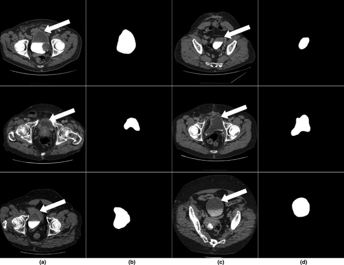
(a,c) Subset of the input computed tomography urography slices containing the bladder (white arrow) used to train the U‐Net–based deep learning approach. (b,d) The corresponding training target binary masks.

The architecture of the 2D U‐DL is illustrated in Fig. 2. This network consisted of a contracting path to capture the context with multiresolution features and a symmetric expanding path to identify the bladder region. The repeated application of two 5 × 5 padded convolutions were used in the contracting path, each convolution layer followed by a rectified linear unit (ReLU) and a 2 × 2 max pooling operation with stride 2 for feature map downsampling. The same padding was applied to the convolution kernels in order to keep the spatial dimensions of the output feature map the same as those of the input feature map, which is a structural difference compared to U‐Net. Each layer in the expanding path consisted of an upsampling of the feature map followed by a 5 × 5 padded convolutions with the ReLU activation function (up‐convolution), repeated application of two 5 × 5 padded convolutions with the ReLU activation function and a concatenation with the correspondingly feature map from the contracting path. The concatenation after two convolution layers was used for better pixel localization, that is, a class label is supposed to be assigned to each pixel. This is another difference from the U‐Net. One more convolutional layer with the ReLU activation function was used and a final 1 × 1 convolution with the sigmoid activation function was applied to map each multicomponent feature vector to the probability of being inside the bladder for each pixel.

Figure 2.

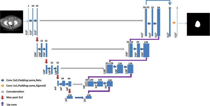
Architecture of the two‐dimensional U‐Net–based deep learning approach for bladder segmentation in computed tomography urography. Each box with number of channels on the top corresponds to a multichannel feature map. The size of each feature map is shown at the lower left edge of the box. The arrows of different colors represent different operations. [Color figure can be viewed at wileyonlinelibrary.com]

2.B.2. 3D U‐DL

In CTU, the consecutive 2D slices constitute a 3D volume. In order to test whether 3D information can facilitate accurate bladder segmentation, we configured a 3D U‐DL structure based on 3D U‐Net²⁶ for bladder segmentation in CTU. Due to the limitation of the GPU memory, we cannot input the entire CTU scan that can exceed 300 slices to the 3D U‐DL. A 3D volume, which consisted of a fixed number of 192 slices, was used as input. The first and the last CTU slice that enclose the bladder marked by radiologist were used to select the 3D volume. The stack of 192 slices was centered automatically in the z dimension between the first and the last slice of the bladder in the CTU volume. If the stack exceeded the CTU scan after the automatic positioning around the bladder, it was shifted to fit inside the CTU scan. The stack of 192 slices was sufficient to enclose the entire bladder for all cases and could fit into the memory of our GPU. The 3D U‐DL was trained with the 3D binary mask of the bladder generated from the manually segmented bladder boundary as expected output. At deployment, the output of 3D U‐DL is the 3D bladder likelihood map of the stack of 192 slices in the CTU volume.

The architecture of the 3D U‐DL is illustrated in Fig. 3. It was composed of a contracting path for context feature extraction and a symmetric expanding path for segmentation mask construction. In the contracting path, each layer contained two 3 × 3 × 3 padded convolutions with the ReLU activation function and a 2 × 2 × 2 max pooling operation with stride 2 for feature map downsampling. The number of feature channels was doubled at each downsampling step of the 3D U‐DL. The same padding was applied to the convolution kernels in order to keep the spatial dimensions of the output feature map the same as those of the input feature map, which is a structural difference compared to U‐Net. Each layer in the expanding path had an up‐convolution, which was concatenated with the correspondingly feature map from the contracting path, followed by two 3 × 3 × 3 padded convolutions with the ReLU activation function. In the last layer a 1 × 1 × 1 convolution with the sigmoid activation function was used to map each multicomponent feature vector to the probability of being inside the bladder for each voxel.

Figure 3.

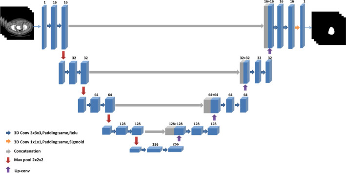
Architecture of the three‐dimensional (3D) U‐Net–based deep learning approach for bladder segmentation in computed tomography urography. Each 3D box with number of channels on the top corresponds to a multichannel 3D feature map. The arrows of different colors represent different operations. [Color figure can be viewed at wileyonlinelibrary.com]

2.B.3. Image downsampling and cropping

To evaluate the effect of image resolution on the U‐DL bladder segmentation, we compared the U‐DL models with input image of different resolutions. The entire original 512 × 512 pixel slice was downsampled to 256 × 256 pixel slice by convolving the original image with a 2 × 2 box filter and downsampling with stride 2. This process essentially increased the pixel size by a factor of 2.

To study the effect of the surrounding background on bladder segmentation, we designed an automated cropping preprocessing procedure and compared the U‐DL models with and without automated cropping preprocessing. In the automated cropping preprocessing, a square region centered at each slice was automatically extracted. The size of the center regions was 256 × 256 pixels for the 512 × 512 pixel images and 128 × 128 pixels for the downsampled 256 × 256 pixel images. The cropped images contained the entire bladder while some surrounding background was removed.

An example of the downsampling and cropping process is shown in Fig. 4. After downsampling or cropping, images of different fields of view or different sizes were generated.

Figure 4.

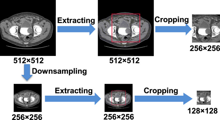
An example of the downsampling and cropping process. [Color figure can be viewed at wileyonlinelibrary.com]

2.B.4. U‐DL training

The U‐DL was trained using the cases in the 81 training/validation dataset. For comparisons of different U‐DL models, images generated by downsampling and/or cropping (Fig. 4) were used as input. The input slice size of the 2D U‐DL may be 512× × 512, 256 × 256, or 128 × 128. The input volume size of the 3D U‐DL may be 256 × 256 × 192 or 128×128 × 192. The dimensions of the U‐DL output bladder likelihood map will correspond to the input image dimensions.

For a U‐DL model and parameter selection, seven cases representative of the different appearances of the bladder in CTU were selected from the 81 training/validation dataset and used as a preliminary validation set. The U‐DL model was trained on the 74 remaining training cases. For each training epoch the U‐DL was deployed on the seven validation cases and the validation results were recorded. The U‐DL parameters resulting in the best validation results were selected. After the final U‐DL model and parameters were selected, the U‐DL was retrained with the whole set of 81 training/validation cases using the selected parameters and then deployed to segment the 92 independent test cases.

During U‐DL training, we used a method for efficient stochastic optimization called Adam²⁷ to optimize the networks by minimizing a binary cross‐entropy cost function. In each training epoch, the training dataset was randomly divided into mini‐batches as input to the U‐DL. We used a Tesla K40c GPU with 12 GB memory to train our models. The 3D U‐DL structure for an input volume size of 512 × 512 × 192 was too large to fit in our GPU memory. The 3D U‐DL structure for an input volume size of 256 × 256 × 192 occupied approximately 11 GB GPU memory so that the batch size was limited to 1. A batch size of 2 was used for the 3D U‐DL model with input volume size of 128 × 128 × 192. For the 2D U‐DL models, we used a batch size of 4. Within each epoch, N (number of training samples/mini‐batch size) iterations were applied. All weights were initialized by a normal distribution with a mean of 0 and a standard deviation of 0.02. The learning rate was selected as 0.0001 based on the training/validation dataset as a good compromise for obtaining a satisfactory accuracy. We have observed that small changes in the learning rate did not influence noticeably the training procedure and the model accuracy. The training was stopped at a fixed number of epochs that was 100 for 2D U‐DL and 400 for 3D U‐DL, for which 2D U‐DL and 3D U‐DL reached convergence for all experiments.

2.B.5. Bladder segmentation using U‐DL bladder likelihood map

For each CTU, the U‐DL models output a bladder likelihood map. Each pixel value of the map indicated the likelihood of the pixel being in the bladder region. A threshold was needed to segment the likelihood map into a binary image with two major regions, one inside and the other outside the bladder. Experimentally, by using the training and validation sets, we selected the threshold to be 0.2. More details about the threshold selection are presented in Section 3.A. After the bladder candidate region was generated, the largest connected component was identified as the bladder region and converted to a binary mask. Then based on the binary mask, the bladder segmentation contour was generated.

2.C. Bladder segmentation using the baseline DCNN‐LS model

We previously developed a bladder segmentation method using deep learning convolution neural network and level sets (DCNN‐LS)²² within a user defined input bounding box. In this study, the DCNN‐LS model was used as the baseline for comparison with our new U‐DL model. Briefly, a DCNN was trained to distinguish between the inside and the outside of the bladder using regions of interest (ROIs) extracted from CTU images and labeled according to their location. The trained DCNN was then used to estimate the likelihood of an ROI being inside the bladder for ROIs centered at each voxel in a CTU volume. Thresholding and hole‐filling were applied to the likelihood map to generate the initial contour for the bladder, which was then refined by 3D and 2D level sets.

2.D. Performance evaluation methods

The bladder segmentation performance was assessed by comparing the computer's segmentation results to the radiologist's 3D hand outlines. In order to quantify the segmentation accuracy, we used quantitative performance measures such as the volume intersection ratio, the volume error, the average minimum distance, the Hausdorff distance,²⁸ and the Jaccard index²⁹ which were estimated between the hand outlines and computer‐segmented contours. The performance measures are defined below and more details can be found in our previous studies.^{16, 22} Let G be the radiologist's reference standard contour, and U be the contour being evaluated. The performance measures are defined as:

• 1 The volume intersection ratio (R ^3D )

$$R^{3D}=\frac{V_G\cap V_U}{V_G}$$

V _G and V _U are the volume enclosed by G and the volume enclosed by U, respectively.

• 2The volume error (E ^3D )

$$E^{3D}=\frac{V_G-V_U}{V_G}$$

The volume error represented the ratio of the difference between the two volumes to the reference volume, which indicates undersegmentation if the value is positive and indicates oversegmentation if the value is negative. In order to show the actual deviations from the reference standard, the absolute error |E ^3D | is also calculated.

• 3The average minimum distance (AVDIST)

$$\begin{array}{cc}\hfill AVDIST=& \frac{1}{2}\left(\frac{{\sum }_{x\in G}min\{d(\mathit{x},\mathit{y}:\mathit{y}\in U)\}}{N_G}\right.\hfill \\ & \left.+\frac{{\sum }_{y\in U}min\{d(\mathit{x},\mathit{y}:\mathit{x}\in G)\}}{N_U}\right)\hfill \end{array}$$

The average minimum distance represented the average of the distances between the closest points of two contours. The number of voxels on G and U are denoted by N _G and N _U , respectively. d denotes the Euclidean distance function. For a given voxel along the contour G, the distance to the closest point along the contour U is determined, and the minimum distances obtained for all points along G are averaged. The process is repeated by switching the roles of G and U and then two average minimum distances are averaged.

• 4The Hausdorff distance (HD)

$$HD=max\left\{\underset{x\in G}{max}\{\underset{y\in U}{min}\{d(\mathit{x},\mathit{y})\}\},\underset{y\in U}{max}\{\underset{x\in G}{min}\{d(\mathit{x},\mathit{y})\}\}\right\}$$

The Hausdorff distance measured the maximum distances between the closest points of two contours.

• 5The Jaccard index (JACCARD ^3D )

$$JACCAR{D}^{3D}=\frac{V_G\cap V_U}{V_G\cup V_U},$$

where it is defined as the ratio of the intersection between V _G and V _U to the union of the V _G and V _U .

Using the measures defined above, the segmentation performance of each case can be quantified relative to the reference standard. The segmentation accuracy on the entire test set was then calculated as the average of each measure over all cases in the set, resulting in the following five summary measures: average volume intersection ratio (AVI), average percent volume error (AVE), average absolute volume error (AAVE), average minimum distance (AMD), average Hausdorff distance (AHD), and the average Jaccard index (AJI).

3. Results

3.A. Threshold selection for U‐DL

The U‐DL models output a likelihood map of the bladder in CTU. A threshold was needed to segment the likelihood map into a binary image. Figure 5 shows an example of the bladder segmentation results using U‐DL from a case in the test set.

Figure 5.

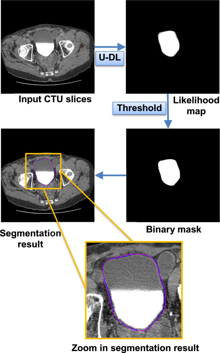
An example of the bladder segmentation results using two‐dimensional (2D) U‐DL with 512 × 512 pixel resolution as input and with automated cropping in preprocessing from a case in the test set. The dark (blue) contour represents the radiologist's hand outline. The lighter (pink) contour represents segmentation using 2D U‐DL with threshold 0.2. [Color figure can be viewed at wileyonlinelibrary.com]

For the likelihood map generated by U‐DL, different thresholds provided slightly different results. In order to select the threshold we compared different threshold results for 2D U‐DL and 3D U‐DL trained on 74 training cases and tested on the 7 selected validation cases. Table 1 summarizes the results with different thresholds on the validation set.

Table 1.

The performance measures results using different threshold on the validation set

Model	Threshold	AVI (%)	AVE (%)	AAVE (%)	AMD (mm)	AHD (mm)	AJI (%)
2D U‐DL	0.1	93.3 ± 7.9	1.0 ± 9.0	5.1 ± 7.2	2.1 ± 1.0	9.1 ± 5.4	88.4 ± 7.6
	0.2	92.3 ± 8.5	3.4 ± 9.3	4.9 ± 8.5	2.0 ± 1.1	9.2 ± 5.9	88.5 ± 8.2
	0.3	91.4 ± 8.9	5.0 ± 9.5	5.6 ± 9.2	2.0 ± 1.1	9.2 ± 5.9	88.3 ± 8.7
	0.4	90.7 ± 9.3	6.3 ± 9.8	6.4 ± 9.7	2.1 ± 1.2	9.4 ± 6.3	88.0 ± 9.1
	0.5	89.9 ± 9.6	7.4 ± 1.0	7.4 ± 1.0	2.1 ± 1.3	9.6 ± 6.4	87.6 ± 9.4
	0.6	89.1 ± 9.9	8.6 ± 10.3	8.6 ± 10.3	2.2 ± 1.4	9.8 ± 6.6	87.2 ± 9.7
	0.7	88.2 ± 10.3	9.9 ± 10.6	9.9 ± 10.6	2.3 ± 1.4	10.1 ± 6.8	86.6 ± 10.1
	0.8	87.1 ± 10.7	11.4 ± 10.9	11.4 ± 10.9	2.4 ± 1.5	10.4 ± 7.0	85.7 ± 10.5
	0.9	85.3 ± 11.3	13.5 ± 11.4	13.5 ± 11.4	2.7 ± 1.6	10.8 ± 7.1	84.4 ± 11.1
3D U‐DL	0.1	92.6 ± 9.7	1.1 ± 11.8	7.1 ± 9.1	2.2 ± 1.1	9.4 ± 5.5	87.1 ± 8.6
	0.2	91.1 ± 11.2	3.9 ± 12.8	6.5 ± 11.5	2.2 ± 1.3	9.8 ± 6.7	86.8 ± 10.2
	0.3	90.0 ± 12.0	5.8 ± 12.0	6.6 ± 12.9	2.3 ± 1.6	10.3 ± 7.6	86.3 ± 11.2
	0.4	89.1 ± 12.4	7.3 ± 13.5	7.4 ± 13.5	2.3 ± 1.6	10.5 ± 7.8	86.0 ± 11.7
	0.5	88.1 ± 12.9	8.8 ± 13.8	8.8 ± 13.8	2.4 ± 1.7	10.8 ± 8.1	85.5 ± 12.2
	0.6	87.1 ± 13.6	10.4 ± 14.4	10.4 ± 14.4	2.5 ± 1.9	11.3 ± 8.9	84.8 ± 13.0
	0.7	86.0 ± 13.8	11.8 ± 14.5	11.8 ± 14.5	2.6 ± 1.9	11.7 ± 9.1	84.1 ± 13.4
	0.8	84.8 ± 14.1	13.4 ± 14.6	13.4 ± 14.6	2.7 ± 1.9	12.1 ± 9.2	83.3 ± 13.7
	0.9	83.1 ± 14.3	15.6 ± 14.7	15.6 ± 14.7	3.0 ± 2.0	12.8 ± 9.5	82.0 ± 14.1

Data are mean ± standard deviation.

AVI: average volume intersection; AVE: average percent volume error; AAVE: average absolute volume error; AMD: average minimum distance; AHD: average Hausdorff distance; AJI: average Jaccard index.

The 512 × 512 pixel resolution and automated cropping preprocessing were used in the U‐Net–based deep learning approach.

Based on the performance measures in Table 1, the best performance was obtained around thresholds of 0.1 or 0.2 for both the 2D and 3D models. We selected the threshold of 0.2 for both U‐DL to be consistent and also to avoid using the somewhat extreme low value of 0.1.

3.B. Comparison of different U‐DL models

In this study, we designed and compared the following U‐DL models for bladder segmentation: (a) 2D U‐DL and 3D U‐DL using 2D CT slices and 3D CT volumes, respectively, as input, (b) U‐DLs using CT images of different resolutions as input, and (c) U‐DLs with and without automated cropping of the bladder as an image preprocessing step.

Initially, we evaluated the segmentation performance by training on the 74 training cases and evaluating on the 7 selected validation cases. Table 2 summarizes the results for the different models in the validation set. Based on the segmentation performance on the validation set, the parameters for the final U‐DL model were selected. The selected model was retrained with the whole set of 81 training/validation cases to maximize the training set and then was deployed to segment the 92 independent test cases. Table 3 summarizes the results for the different models on the independent test set.

Table 2.

The performance measures using different models on the validation set

Model	Resolution	Cropping	AVI (%)	AVE (%)	AAVE (%)	AMD (mm)	AHD (mm)	AJI (%)
2D U‐DL	512 × 512	With	92.3 ± 8.5	3.4 ± 9.3	4.9 ± 8.5	2.0 ± 1.1	9.2 ± 5.9	88.5 ± 8.2
		Without	92.8 ± 7.9	1.2 ± 8.8	5.5 ± 6.7	3.0 ± 2.6	10.7 ± 5.6	87.6 ± 8.0
	256 × 256	With	91.9 ± 11.7	2.3 ± 14.4	7.7 ± 12.0	2.5 ± 1.5	10.1 ± 6.8	86.8 ± 10.4
		Without	91.0 ± 10.7	2.4 ± 12.5	7.0 ± 10.4	2.4 ± 1.2	10.4 ± 6.3	85.5 ± 9.9
3D U‐DL	512 × 512	With	91.1 ± 11.2	3.9 ± 12.8	6.5 ± 11.5	2.2 ± 1.3	9.8 ± 6.7	86.8 ± 10.2
		Withouta	–	–	–	–	–	–
	256 × 256	With	88.6 ± 12.8	2.0 ± 16.8	10.8 ± 12.3	3.1 ± 1.5	13.5 ± 7.9	81.2 ± 11.8
		Without	90.1 ± 14.4	3.5 ± 16.2	8.9 ± 13.5	2.4 ± 1.5	10.3 ± 8.0	84.7 ± 13.4

Data are mean ± standard deviation.

AVI: average volume intersection; AVE: average percent volume error; AAVE: average absolute volume error; AMD: average minimum distance; AHD: average Hausdorff distance; AJI: average Jaccard index.

^aThe input of three‐dimensional U‐DL with 192 512 × 512 pixel slices was too big to fit in our GPU.

Table 3.

The performance measures using different models on the independent test set

Model	Resolution	Cropping	AVI (%)	AVE (%)	AAVE (%)	AMD (mm)	AHD (mm)	AJI (%)
2D U‐DL	512 × 512	With	93.4 ± 9.5	−4.2 ± 14.2	9.2 ± 11.5	2.7 ± 2.5	9.7 ± 7.6	85.0 ± 11.3
		Without	93.0 ± 9.8	−3.0 ± 13.9	8.9 ± 11.1	2.7 ± 2.6	9.9 ± 8.0	85.1 ± 10.9
	256 × 256	With	92.9 ± 9.8	−3.1 ± 13.2	9.3 ± 9.8	2.8 ± 2.4	10.0 ± 7.1	84.5 ± 10.0
		Without	93.6 ± 9.5	−5.7 ± 14.2	10.7 ± 10.9	2.9 ± 2.6	10.3 ± 7.5	84.0 ± 10.6
3D U‐DL	512 × 512	With	90.6 ± 11.9	−2.3 ± 21.7	11.5 ± 18.5	3.1 ± 3.2	11.4 ± 10.0	82.6 ± 14.2
		Withouta	–	–	–	–	–	–
	256 × 256	With	89.1 ± 13.1	−0.6 ± 19.5	11.9 ± 15.4	3.4 ± 3.1	11.7 ± 8.8	80.8 ± 13.4
		Without	90.1 ± 14.6	−3.1 ± 24.5	13.3 ± 20.8	3.3 ± 3.2	11.5 ± 10.1	81.1 ± 15.7

Data are mean ± standard deviation.

AVI: average volume intersection; AVE: average percent volume error; AAVE: average absolute volume error; AMD: average minimum distance; AHD: average Hausdorff distance; AJI: average Jaccard index; 2D U‐DL: two‐dimensional U‐Net–based deep learning approach; 3D U‐DL: three‐dimensional U‐Net–based deep learning approach.

^aThe input of three‐dimensional U‐DL with 192 512 × 512 pixel slices was too big to fit in our GPU.

As shown in Table 2, for the same conditions of image resolution and preprocessing, the 2D U‐DL always performed better than 3D U‐DL. Similar trends were observed in the Table 3 when the U‐DL models were tested on the independent test set.

For different image resolution, we compared images with 512 × 512 pixels to 256 × 256 pixels in the same conditions of input dimension and preprocessing. The U‐DL segmentation of the full resolution images with 512 × 512 pixels was always slightly better than the downsampled 256 × 256 pixel images on the validation set. Similar trends were observed when the U‐DL models were tested on the independent test set.

For the comparison of preprocessing with and without automated cropping on each slice, the results of U‐DL segmentation were similar for the same conditions of image resolution and preprocessing on the validation set. Also, similar trends were observed when the U‐DL models were tested on the independent test set.

Although the segmentation performances were similar, the preprocessing with automated cropping was able to reduce the computation time of training. The computation time of training an epoch for different U‐DL models are shown in Table 4. Since preprocessing with automated cropping was able to save computation time of training, we used the automated cropping for the final U‐DL model.

Table 4.

The computation time of training an epoch for two‐dimensional (2D) and an epoch for three‐dimensional (3D) for different U‐Net–based deep learning approach (U‐DL) models

Model	Resolution	Cropping	Computation time (min)
2D U‐DL	512 × 512	With	18.5
		Without	70.0
	256 × 256	With	5.8
		Without	49.5
3D U‐DL	512 × 512	With	32.5
		Withouta	–
	256 × 256	With	10
		Without	29

^aThe input of 3D U‐DL with 192 512 × 512 pixel slices was too big to fit in our GPU.

Overall, the best U‐DL model for bladder segmentation was the 2D U‐DL model with 512 × 512 pixel resolution and automated cropping.

3.C. 2D U‐DL and 3D U‐DL vs baseline DCNN‐LS

We compared the 2D U‐DL and 3D U‐DL with our previous developed DCNN‐LS method that was based on DCNN and level sets (DCNN‐LS) within a user‐input bounding box. From the comparison of different U‐DL models, we observed that using input images of 512 × 512 pixel resolution and automated cropping were better for both the 2D and the 3D U‐DL bladder segmentation models. Table 5 summarized the results using the best 2D U‐DL, the best 3D U‐DL, and the DCNN‐LS methods on the independent test set. The improvement in all performance measures by the best 2D U‐DL model compared to the DCNN‐LS model was statistically significant (P < 0.001). The differences in AVI, AVE, and AJI by the best 3D U‐DL model compared to DCNN‐LS model were also statistically significant (P < 0.001). The differences in AVI, AMD, AHD, and AJI by the best 2D U‐DL model compared to the best 3D U‐DL model were statistically significant (P < 0.006).

Table 5.

The performance measures results using the best two‐dimensional (2D) U‐Net–based deep learning approach (U‐DL), the best three‐dimensional (3D) U‐DL and the deep learning convolution neural network and level sets methods on the independent test set

Model	AVI (%)	AVE (%)	AAVE (%)	AMD (mm)	AHD (mm)	AJI (%)
2D U‐DL	93.4 ± 9.5	−4.2 ± 14.2	9.2 ± 11.5	2.7 ± 2.5	9.7 ± 7.6	85.0 ± 11.3
3D U‐DL	90.6 ± 11.9	−2.3 ± 21.7	11.5 ± 18.5	3.1 ± 3.2	11.4 ± 10.0	82.6 ± 14.2
DCNN‐LS	81.9 ± 12.1	10.2 ± 16.2	14.0 ± 13.0	3.6 ± 2.0	12.8 ± 6.1	76.2 ± 11.8

Data are mean ± standard deviation.

AVI: average volume intersection; AVE: average percent volume error; AAVE: average absolute volume error, AMD: average minimum distance; AHD: average Hausdorff distance; AJI: average Jaccard index.

The histograms of the best 2D and 3D results compared to the DCNN‐LS baseline model are shown in Fig. 6.

Figure 6.

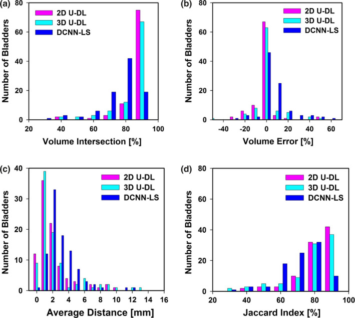
Histograms of (a) volume intersection (mean: two‐dimensional (2D) U‐Net–based deep learning approach (U‐DL) = 93.4 ± 9.5%, three‐dimensional (3D) U‐DL = 90.6 ± 11.9%, deep learning convolution neural network and level sets (DCNN‐LS) = 81.9 ± 12.1%), (b) volume error (mean: 2D U‐DL = −4.2 ± 14.2%, 3D U‐DL = −2.3 ± 21.7%, DCNN‐LS = 10.2 ± 16.2%), (c) average distance (mean: 2D U‐DL = 2.7 ± 2.5 mm, 3D U‐DL = 3.1 ± 3.2 mm, DCNN‐LS = 3.6 ± 2.0 mm), (d) Jaccard index (mean: 2D U‐DL = 85.0 ± 11.3%, 3D U‐DL = 82.6 ± 14.2%, DCNN‐LS = 76.2 ± 11.8%), for the 92 test cases. [Color figure can be viewed at wileyonlinelibrary.com]

3.D. U‐DL vs nondeep learning (non‐DL) methods

We compared the U‐DL with two non‐DL methods, the conjoint level set analysis and segmentation system with local contour refinement (CLASS‐LCR) method³⁰ and the level sets method using Haar feature‐based likelihood map (LS‐HF) method.²² Most existing non‐DL methods for bladder segmentation were based on level set algorithm. The CLASS‐LCR was further developed from the CLASS method, which had been shown to be more accurate than an edge‐based level set method.¹⁶ All methods were evaluated relative to the 3D hand‐segmented reference contours. Table 6 summarized the results using the best 2D U‐DL, the best 3D U‐DL, the CLASS‐LCR, and the LS‐HF methods on the independent test set. It was found that the 2D and 3D U‐DL methods were better than the two non‐DL methods for all performance measures.

Table 6.

The performance measures results using the best two‐dimensional (2D) U‐Net–based deep learning approach (U‐DL), the best three‐dimensional (3D) U‐DL, the conjoint level set analysis and segmentation system with local contour refinement (CLASS‐LCR) and the LS‐HF on the independent test set

Model	AVI (%)	AVE (%)	AAVE (%)	AMD (mm)	AHD (mm)	AJI (%)
2D U‐DL	93.4 ± 9.5	−4.2 ± 14.2	9.2 ± 11.5	2.7 ± 2.5	9.7 ± 7.6	85.0 ± 11.3
3D U‐DL	90.6 ± 11.9	−2.3 ± 21.7	11.5 ± 18.5	3.1 ± 3.2	11.4 ± 10.0	82.6 ± 14.2
CLASS‐LCR	78.0 ± 14.7	16.5 ± 16.8	18.2 ± 15.0	3.8 ± 2.3	13.1 ± 6.2	73.9 ± 13.5
LS‐HF	74.3 ± 12.7	13.0 ± 22.3	20.5 ± 15.7	5.7 ± 2.6	16.8 ± 7.5	66.7 ± 12.6

Data are mean ± standard deviation.

AVI: average volume intersection; AVE: average percent volume error; AAVE: average absolute volume error; AMD: average minimum distance; AHD: average Hausdorff distance; AJI: average Jaccard index.

4. Discussion

In this study, a new approach of using U‐DL for segmenting bladders in CTU was developed. On excretory phase CTU images, as performed at our institution, most bladders are either partially or entirely filled with excreted contrast material; however, occasional bladders do not contain any contrast‐enhanced urine. Segmentation of these variably opacified bladders is a challenge because the segmentation may need to cross portions of the bladder that are opacified and portions that are not opacified. Previously, we used DCNN‐LS within a user defined input bounding box to alleviate the problem. However, the user defined input bounding box is no longer needed using the newly developed U‐DL approach. The contribution of this work is that it investigated different conditions to construct better U‐DL model and the results demonstrate that the selected U‐DL is more accurate and does not depend on a user‐input bounding box compared to the previous DCNN‐LS method on a validation set and an independent test set. All performance measures are improved using U‐DL compared to DCNN‐LS for the independent test set. The differences between the U‐DL and DCNN‐LS methods are statistically significant (P < 0.001).

By examining the results, we observed that the U‐DL performs better than the DCNN‐LS methods in most situations. Figure 7 shows examples of segmented bladders using the different models.

Figure 7.

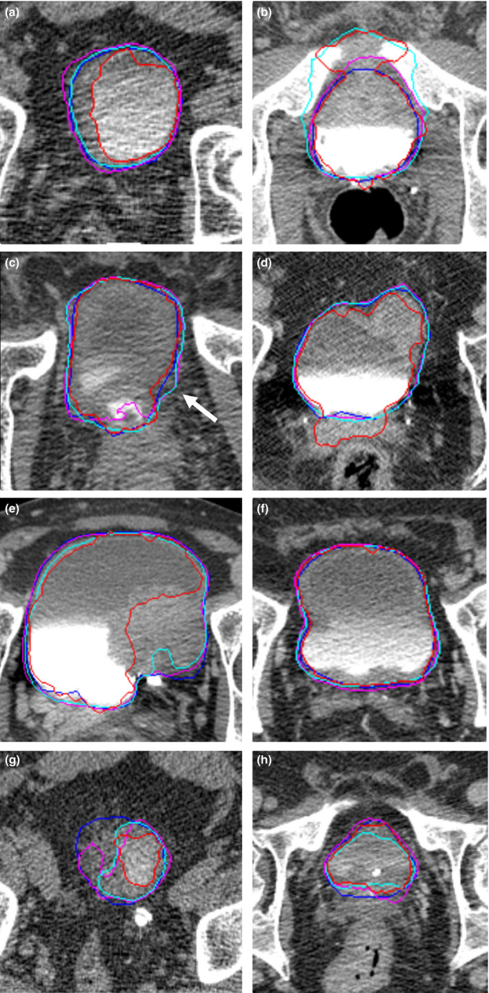
Examples of bladder segmentation. The light (cyan) contour represents segmentation using three‐dimensional (3D) U‐Net–based deep learning approach (U‐DL). The darker (pink) contour represents segmentation using two‐dimensional (2D) U‐DL. The darkest (red) contour represents segmentation using deep learning convolution neural network and level sets (DCNN‐LS). The darkest (blue) contour represents the radiologist's hand outline. (a) 2D U‐DL and 3D U‐DL performed better in the case with poor image quality, where DCNN‐LS undersegmented the bladder. (b) DCNN‐LS and 3D U‐DL leaked into adjacent bones, but 2D U‐DL was able to avoid the leaking. (c) 2D U‐DL undersegmented the contrast area at the bottom of the bladder. 2D and 3D U‐DL oversegmented the bladder boundary near the middle of the bladder (white arrow). (d) DCNN‐LS oversegmented the contrast area at the bottom of the bladder. 2D and 3D U‐DL provided good segmentation. (e) DCNN‐LS undersegmented the bladder lesion. 2D and 3D U‐DL provided good segmentation. (f) Both DCNN‐LS and U‐DL provided good segmentation. (g) DCNN‐LS, 2D U‐DL, and 3D U‐DL undersegmented the bladder. (h) DCNN‐LS, 2D U‐DL, and 3D U‐DL provided relative relatively good segmentation. [Color figure can be viewed at wileyonlinelibrary.com]

Both DCNN‐LS and U‐DL were able to provide good segmentation in relatively simple cases [Fig. 7(f)]. However, there are some difficult cases in our dataset. Several of them were of poor image quality due to noise caused by large patient size or the presence of hip prostheses. An example of such as case is shown in Fig. 7(a), 2D U‐DL and 3D U‐DL performed better in this case, where DCNN‐LS undersegmented the bladder. The strong boundary between the two regions filled with intravenous contrast and without contrast impacted the segmentation performance. Figure 7(b) shows that DCNN‐LS– and 3D U‐DL–created bladder outlines have leaked into adjacent bones because of a strong boundary between the opacified and unopacified portions of the bladder and the bones and the unopacified portions of the bladder. The 2D U‐DL–generated outline was able to avoid this erroneous leak. Furthermore, the boundaries between the bladder wall and the surrounding soft tissue are difficult to identify because of the small difference in gray level. As observed in Fig. 7(c), the DCNN‐LS method was able to avoid the leakage between the bladder wall and the surrounding soft tissue but not in Fig. 7(d), while U‐DL was slightly leaking in Fig. 7(c) but was able to avoid the leakage in Fig. 7(d). Usually the lesion area of the bladder had similar gray levels as the surrounding soft tissue, which may cause inaccurate segmentation. As shown in Fig. 7(e), DCNN‐LS undersegmented the lesion area of the bladder while 2D and 3D U‐DL provided good segmentation. The apex and the base of the bladder usually were difficult to segment due to the small bladder area, irregular bladder boundary intersecting the CT slice and reduced bladder contrast due to partial volume effects. Figure 7(g) shows that DCNN‐LS, 2D U‐DL, and 3D U‐DL undersegmented the apex of the bladder while Fig. 7(h) shows that they provided relatively good segmentation for the base of the bladder.

Although U‐DL provided accurate bladder segmentation in the majority of cases, there were several cases in the independent test dataset for which the segmentation was suboptimal. For the best U‐DL model, 2 of the 92 cases achieved volume intersection ratio less than 50% which may be considered for a major contour adjustment. Three of the 92 cases achieved a volume intersection ratio between 50% and 80% which may be considered for a minor adjustment.

When 3D U‐DL was used instead of 2D U‐DL, performance measures generally deteriorated in the bladder segmentation task. One possible reason may be that the training sample size was small when 3D volumes were used as an input. The number of the input samples was 81 for 3D U‐DL compared to 7629 for 2D U‐DL. Generally, the training of DCNN model needs a large amount of labeled data.

When the full resolution images with 512 × 512 pixels were used as input for the U‐DL model, the segmentation performances were always slightly better than the downsampled 256 × 256 pixel images on both the validation set and independent test set. Higher resolution can provide more detailed information. However, compared to 512 × 512 pixel images, using images with 256 × 256 pixels reduced the computation time of training by about a factor of 2 to 3 (Table 4). Nonetheless, we chose full resolution images with 512 × 512 pixels for the U‐DL model because the accurate performance was more important than the computation time of training in this task.

When we applied automated cropping on each slice in the preprocessing, the segmentation performances of U‐DL were similar to preprocessing without automated cropping on the validation set and the independent test set. The cropped images still contained the entire bladder but removed some surrounding background. The surrounding background farther away from the bladder boundary did not provide an important feature for bladder segmentation. Although the segmentation performances were similar, the preprocessing with automated cropping reduced the computation time of training (Table 4).

We also investigated the correlation between the segmentation error and the bladder volume. We calculated the Pearson correlation coefficients between the bladder volume enclosed by the hand outlines and the quantitative performance measures for the best U‐DL model. The Pearson correlation coefficients between AVI, AVE, AAVE, AMD, AHD, AJI and the bladder volume were −0.188, 0.364, 0.003, 0.041, 0.107 and 0.052, respectively, for the test set. The results indicated a slight correlation only between AVE and bladder volume.

It was found that the 3D hand outlines may also show a noticeable difference in superior–inferior direction for some consecutive slices because the radiologist drew the boundary of the bladder slice by slice, especially at locations with unclear bladder boundary or adjacent anatomical structures. Since the 2D U‐DL was trained by the hand‐outlines and segmented slice by slice, it is possible that the 2D U‐DL segmentation yields discontinuous contours in the superior–inferior direction for some difficult cases. For 3D U‐DL, the continuity is better than for the 2D U‐DL.

There are some major differences between our study and the study reported in Ref. 23. In Ref. 23, the authors used a small test set of 24 cases while in our study the test set consisted of 92 cases. The bladders in Ref. 23 were imaged with noncontrast‐enhanced CT, while in our experiments the bladders were partially or entirely filled with excreted contrast material or without any contrast material, which makes the segmentation more challenging as discussed above. We did not apply preprocessing of the CT images (such as enhancement density filters) or contour refinement of the U‐DL contour. In addition, we compared both 2D‐ and 3D‐based U‐DL segmentation while reference²³ only studied 3D segmentation.

A limitation of our newly developed approach is that it still needs the user to mark the first and the last slice enclosing the bladder for each unknown case. Nevertheless, this user input may not be necessary if the GPU memory and processing time are not concerns and if the U‐DL model is retrained with the entire CTU scan. One reason for this was that our current GPU does not have enough memory to process the entire CTU scan that can exceed 300 slices. With this limitation, we could not evaluate whether the U‐DL may learn to segment the bladder from the volume automatically by training with a binary mask for the entire CTU volume. However, the user defined input bounding box was no longer needed for U‐DL approach compared to DCNN‐LS. As a result, the U‐DL was more automated than the previous approach. We intend to study a fully automated bladder segmentation method as a next step. Another limitation is that although we have a larger dataset than most of the other studies for bladder segmentation, the dataset is still small for the DCNN training. We will continue to enlarge our dataset to further improve DCNN performance.

5. Conclusion

We have developed a U‐DL method for bladder segmentation in CTU. Compared to our previous DCNN‐LS method, which depended on an user‐input bounding box, the U‐DL provided more accurate bladder segmentation and was more automated than the previous approach. Further work is underway to fully automate the segmentation process and to improve the segmentation accuracy.

Conflict of interest

The authors have no conflicts to disclose.

References

- 1. American Cancer Society . Key Statistics for Bladder Cancer; 2018. www.cancer.org
- 2. Caoili EM, Cohan RH, Korobkin M, et al. Urinary tract abnormalities: initial experience with multi–detector row CT urography. Radiology. 2002;222:353–360. [DOI] [PubMed] [Google Scholar]
- 3. Gupta R, Raghuvanshi S. Multi–detector CT urography in the diagnosis of urinary tract abnormalities. Int J Med Res Rev. 2016;4:222–226. [Google Scholar]
- 4. Akbar SA, Mortele KJ, Baeyens K, Kekelidze M, Silverman SG. Multidetector CT urography: techniques, clinical applications, and pitfalls. Semin Ultrasound CT MRI. 2004;25:41–54. [DOI] [PubMed] [Google Scholar]
- 5. Noroozian M, Cohan RH, Caoili EM, Cowan NC, Ellis JH. Multislice CT urography: state of the art. Br J Radiol. 2004;77:S74–S86. [DOI] [PubMed] [Google Scholar]
- 6. Park SB, Kim JK, Lee HJ, Choi HJ, Cho K‐S. Hematuria: portal venous phase multi–detector row CT of the bladder—a prospective study. Radiology. 2007;245:798–805. [DOI] [PubMed] [Google Scholar]
- 7. Sudakoff GS, Dunn DP, Guralnick ML, Hellman RS, Eastwood D, See WA. Multidetector computerized tomography urography as the primary imaging modality for detecting urinary tract neoplasms in patients with asymptomatic hematuria. J Urol. 2008;179:862–867. [DOI] [PubMed] [Google Scholar]
- 8. Cha KH, Hadjiiski L, Chan HP, Cohan RH, Caoili EM, Zhou C. Detection of urinary bladder mass in CT urography with SPAN. Med Phys. 2015;42:4271–4284. [DOI] [PMC free article] [PubMed] [Google Scholar]
- 9. Cha KH, Hadjiiski L, Chan HP, et al. Bladder cancer treatment response assessment in CT using radiomics with deep‐learning. Sci Rep. 2017;7:12. [DOI] [PMC free article] [PubMed] [Google Scholar]
- 10. Duan C, Liang Z, Bao S, et al. A coupled level set framework for bladder wall segmentation with application to MR cystography. IEEE Trans Med Imaging. 2010;29:903–915. [DOI] [PMC free article] [PubMed] [Google Scholar]
- 11. Chi JW, Brady M, Moore NR, Schnabel JA. Segmentation of the bladder wall using coupled level set methods. Paper presented at: 2011 IEEE International Symposium on Biomedical Imaging: From Nano to Macro; 30 March‐2 April 2011, 2011.
- 12. Han H, Li L, Duan C, Zhang H, Zhao Y, Liang Z. A unified EM approach to bladder wall segmentation with coupled level‐set constraints. Med Image Anal. 2013;17:1192–1205. [DOI] [PMC free article] [PubMed] [Google Scholar]
- 13. Qin X, Li X, Liu Y, Lu H, Yan P. Adaptive shape prior constrained level sets for bladder MR image segmentation. IEEE J Biomed Health Inform. 2014;18:1707–1716. [DOI] [PubMed] [Google Scholar]
- 14. Xu X‐P, Zhang X, Liu Y, et al. Simultaneous segmentation of multiple regions in 3D bladder MRI by efficient convex optimization of coupled surfaces. In: Zhao Y, Kong X, Taubman D, eds. Image and Graphics. Cham: Springer; 2017. [Google Scholar]
- 15. Chai X, Herk MV, Betgen A, Hulshof M, Bel A. Automatic bladder segmentation on CBCT for multiple plan ART of bladder cancer using a patient‐specific bladder model. Phys Med Biol. 2012;57:3945. [DOI] [PubMed] [Google Scholar]
- 16. Hadjiiski L, Chan H‐P, Cohan RH, et al. Urinary bladder segmentation in CT urography (CTU) using CLASS. Med Phys. 2013;40:111906. [DOI] [PMC free article] [PubMed] [Google Scholar]
- 17. Krizhevsky A, Sutskever I, Hinton GE. ImageNet classification with deep convolutional neural networks. Comm ACM. 2012;60:84–90. [Google Scholar]
- 18. Lo SB, Lou SA, Jyh‐Shyan L, Freedman MT, Chien MV, Mun SK. Artificial convolution neural network techniques and applications for lung nodule detection. IEEE Trans Med Imaging. 1995;14:711–718. [DOI] [PubMed] [Google Scholar]
- 19. Chan H‐P, Lo S‐CB, Sahiner B, Lam KL, Helvie MA. Computer‐aided detection of mammographic microcalcifications: pattern recognition with an artificial neural network. Med Phys. 1995;22:1555–1567. [DOI] [PubMed] [Google Scholar]
- 20. Lo S‐CB, Chan H‐P, Lin J‐S, Li H, Freedman MT, Mun SK. Artificial convolution neural network for medical image pattern recognition. Neural Netw. 1995;8:1201–1214. [Google Scholar]
- 21. Sahiner B, Chan H‐P, Petrick N, et al. Classification of mass and normal breast tissue: a convolution neural network classifier with spatial domain and texture images. IEEE Trans Med Imaging. 1996;15:598–610. [DOI] [PubMed] [Google Scholar]
- 22. Cha KH, Hadjiiski L, Samala RK, Chan H‐P, Caoili EM, Cohan RH. Urinary bladder segmentation in CT urography using deep‐learning convolutional neural network and level sets. Med Phys. 2016;43:1882–1896. [DOI] [PMC free article] [PubMed] [Google Scholar]
- 23. Xu X, Zhou F, Liu B. Automatic bladder segmentation from CT images using deep CNN and 3D fully connected CRF‐RNN. Int J Comput Assist Radiol Surg. 2018;13:967–975. [DOI] [PubMed] [Google Scholar]
- 24. Ronneberger O, Fischer P, Brox T. U‐net: convolutional networks for biomedical image segmentation. In: Navab N, Hornegger J, Wells W, Frangi A, eds. Medical Image Computing and Computer‐Assisted Intervention – MICCAI 2015. Cham: Springer; 2015. [Google Scholar]
- 25. Keras CF. GitHub repository; 2015. https://github.com/fchollet/keras
- 26. Çiçek Ö, Abdulkadir A, Lienkamp SS, Brox T, Ronneberger O. 3D U‐net: learning dense volumetric segmentation from sparse annotation. In: Ourselin S, Joskowicz L, Sabuncu M, Unal G, Wells W, eds. Medical Image Computing and Computer‐Assisted Intervention – MICCAI 2016. Cham: Springer; 2016. [Google Scholar]
- 27. Kingma D, Ba J. Adam: a method for stochastic optimization; 2014.
- 28. Rockafellar RT, Wets RJ‐B. Variational Analysis. Vol. 317. Berlin: Springer‐Verlag; 2005:117. [Google Scholar]
- 29. Jaccard P. The Distribution of the Flora in the alpine zone. 1. New Phytol. 1912;11:37–50. [Google Scholar]
- 30. Cha K, Hadjiiski L, Chan H‐P, Caoili EM, Cohan RH, Zhou C. CT urography: segmentation of urinary bladder using CLASS with local contour refinement. Phys Med Biol. 2014;59:2767–2785. [DOI] [PMC free article] [PubMed] [Google Scholar]