Abstract.
Distance correlation is a measure that can detect both linear and nonlinear associations. However, applying distance correlation to imaging genetic studies often needs multiple testing correction due to the large number of multiple inferences. As a result, the sensitivity of its detection may be low. We propose a new model, distance canonical correlation analysis (DCCA), which overcomes this problem by searching a combination of features with the highest distance correlation. This is achieved by constructing a distance kernel function followed by solving a subsequent optimization problem. The ability to detect both linear and nonlinear associations makes DCCA suitable for analyzing complex multimodal and imaging-genetic associations. When applied to a brain imaging-genetic study from the Philadelphia Neurodevelopmental Cohort (PNC), DCCA detected several mental disorder-related gene pathways and brain networks. Experiments on brain connectivity found that the default mode network had strong nonlinear connections with other brain networks. When applied to the study of age effects, DCCA revealed that the connections of brain networks were relatively weak in younger groups but became stronger at older age stages. It indicates that adolescence is a vital stage for brain development. DCCA thus reveals a number of interesting findings and demonstrates a powerful new approach for analyzing multimodal brain imaging data.
Keywords: distance correlation, nonlinear, multimodal, functional magnetic resonance imaging, imaging genetics, brain networks
1. Introduction
The brain is a complex organ and investigating its development and relationship with genomics is of great interest. Advances in neuroimaging, e.g., functional magnetic resonance imaging (fMRI), and sequencing of genetic variations, e.g., singular nucleotide polymorphism (SNP), have facilitated the analysis of the relationship between brain regions and genetic variations. FMRI detects changes in functional brain activity at each voxel, which can be clustered into regions of interest (ROI). SNPs are important genetic factors underlying differences in phenotypes among human beings. Association analyses, e.g., canonical correlation analysis (CCA),1 have been conducted to study brain connectivity and how genetic factors and endophenotypes interact.2 However, these methods typically use Pearson correlation which only captures linear relationships while nonlinear correlations may exist among brain regions.3
To address the limitation of Pearson correlation-based methods, Székely et al.4 proposed a correlation measurement, distance correlation, which evaluates the dependence between two single variables or two sets of variables. The property that distance correlation equals 0 if and only if two variables are independent enables it to detect both linear and nonlinear associations. Besides the ability to detect nonlinear correlations, the flexibility to detect both single-single feature correlations and set–set feature correlations also help distance correlation find many applications in imaging genetic and brain connectivity study. Geerligs et al.5 investigated the dependence between different ROIs using multivariate distance correlation and the results tended to be more robust than using Pearson correlation. Fang et al.6 investigated complex imaging genetics associations using projected distance correlation, which was more accurate and fast.
Székely and Rizzo7 constructed a statistic to evaluate the statistical significance of the distance correlation between two single or two sets of variables. Despite the well-constructed theoretical work, a challenge for applying distance correlation exists in multiple testing correction. Large-scale simultaneous inference testing, e.g., genome wide association study (GWAS), needs multiple testing correction, e.g., Bonferroni correction,8 in order to prevent erroneous inferences. For distance correlation, the scale of simultaneous inference is (, are variable sizes of two datasets), which is much larger than that of GWAS, i.e., . As a result, it might be difficult to detect significant variable–variable distance correlations due to the harsher testing correction. For testing the distance correlation between two subsets of variables, the scale of multiple inference testing is even larger, i.e., , and consequently the detection of significant associations becomes even more difficult.
To address the challenge, we propose a new framework, distance canonical correlation analysis (DCCA), which overcomes the problem by searching a combination of original features with the highest distance correlation. It is achieved by first constructing a distance kernel function and then solving a subsequent optimization problem. In this way, DCCA can detect both linear and nonlinear correlations and can identify a subset of features that are significantly correlated.
This work is an expansion of a preliminary work, “A hybrid correlation analysis with application to imaging genetics,”9 which was published in the proceedings of SPIE Medical Imaging 2018. This work refines the conference paper by adding more detailed procedures about the method and more applications on both the fusion of imaging genetics data and the fusion of multiple brain imaging data. The rest of this paper is organized as follows. Section 2 first introduces distance correlation with pros and cons and then discusses how the proposed model, DCCA, can overcome the limitation. Section 3 presents a simulation experiment test to verify the performance of DCCA. Section 4 presents the collection and preprocessing of data as well as the experiments of applying DCCA to detecting imaging genetic associations and brain connectivity study. Discussion and conclusions are in Sec. 5.
2. Methods
2.1. Distance Correlation
Distance correlation, proposed by Székely et al.,4 measures the dependence between two single variables or two sets of variables. Suppose we have two sets of random variables and (where , represent the feature sizes of , , respectively) with characteristic functions and . Variable dimensionality , can either be 1 (two single variable case) or greater than 1 (two sets of variables case). The distance covariance between and is defined as
| (1) |
where , denote the Euclidean norm in space and , respectively; and denotes the joint characteristic function of and .
The distance correlation between and is defined as
| (2) |
It has been proved that distance correlation gets 0 iff and are independent, i.e.,
| (3) |
Distance correlation outperforms conventional Pearson correlation in that it can detect both linear and nonlinear associations due to Eq. (3).
For sample data and , where denotes sample size, the empirical distance covariance between and can be estimated as follows. First, we calculate the Euclidean distance between each sample pair
Second, U-centering is applied to the Euclidean distance as
| (4) |
The U-centered can be calculated similarly, i.e., applying U-centering to Euclidean distance . Then, the empirical distance correlation can be calculated as
| (5) |
A statistic following a -distribution provided by Székely and Rizzo7 is used to evaluate the significance of distance correlation as
| (6) |
2.2. Kernel Methods
Kernel methods are also widely used when data have nonlinear relationships. Kernel methods map original variable space to a higher dimensional space ( can be either or a number greater than ) via a mapping function as
| (7) |
In order to reduce computational complexity and to avoid computing in , kernel trick is used to compute with a kernel function instead of an explicit mapping function. A kernel function is defined as
| (8) |
where , are two samples and denotes the inner product in space.
2.3. Distance Canonical Correlation Analysis
Distance correlation provides a way to evaluate the dependence between two single variables or two sets of variables. Given two datasets and , it is of interest to identify which two single variables and are significantly dependent by computing their distance correlation. However, it may be difficult to detect significant distance correlations due to multiple testing correction. Multiple testing correction, e.g., Bonferroni correction,8 is used to counteract the problem of multiple comparisons when conducting a large scale of statistical inference simultaneously, e.g., GWAS. For GWAS study, the scale of simultaneous inference is the variable/feature size . For univariate distance correlation (distance correlation between two single variables), the scale of simultaneous inference is , which is much larger than that of GWAS, i.e., .
In data application, it is usually of interest to study groups of variables rather than a single feature. For examples, complex phenotypes and diseases may be regulated by a group of genes and pathways. For brain imaging data, different brain regions function and harmonize in a connected network when performing a specific brain function.10 Therefore, it is of interest to identify two subsets/groups of variables and which are significantly dependent. However, the scale of simultaneous inference in this case is very large, i.e., , making it more difficult to detect significantly dependent subsets.
Motivated by the problem in detecting significant distance correlation, we develop a multivariate approach, namely DCCA, to seek the optimal combination of original variables with the highest distance correlations. Given two datasets and , distance CCA first projects original samples to a higher dimensional space as in the following procedure.
For any two single features , from data , a distance kernel is defined as
| (9) |
where , denote the ’th and ’th elements of , respectively; and the corresponding mapping function is
| (10) |
where , (, mod ).
It is easy to check that Eq. (9) is a well-defined inner product in a reproducing kernel Hilbert space. With distance kernel constructed, a multivariate method is used to find the optimal combination of original features/variables with the highest distance correlation by solving the optimization problem as
| (11) |
where , , , , ; denotes the ’th element of ; and , denote the ’th column of , , respectively.
The detailed algorithm for the proposed model, DCCA, and the detailed procedures of solving the optimization problem [Eq. (11)] are described in Algorithm 1.
Algorithm 1.
Algorithm for DCCA.
| 1: Input, , initial loading vectors , |
| 2: Output Optimal loading vectors , |
| 3: Construct distance kernel Gram matrices |
| 4: |
| 5: |
| 6: |
| 7: U-centering: |
| 8: Solve optimization problem [Eq. (11)] |
| 9: |
| 10: |
| 11: return, |
The framework of distance CCA is similar to that of kernel CCA, which is another nonlinear methods, and therefore we call the constructed Gram matrix [Eqs. (9) and (10)] “distance kernel.” However, it is noteworthy that distance CCA differs from conventional kernel CCA and cannot be regarded as kernel CCA with a newly defined kernel function. For kernel CCA, there are a number of options for kernel functions, e.g., Gaussian radial basis function kernel, polynomial kernel, etc. The choice of kernel function depends on data distributions and the hidden relationship pattern within the data. Distance kernel function [Eqs. (9) and (10)] differs from conventional kernel function in that distance kernel retains the original feature information [for , distance kernel operation ] while conventional kernel function breaks the original feature structure [for , kernel operation ]. The retaining of original feature structure enables distance CCA to perform feature selection which can facilitate subsequent result interpretation. In comparison, it is difficult to interpret the result of kernel CCA since the original feature information is lost after kernel mapping.
3. Simulation Test
To illustrate the strengths and limitations of our method, namely DCCA, we conducted a simulation study and compared the performances of DCCA to that of linear CCA. For performance comparison, two aspects were considered: correlation detection and feature selection.
3.1. Synthetic Data
We employed a latent variable model,11 also used in works,12,13 to simulate two correlated data , , where represents sample/subject size, and , represent feature size. Suppose we have two latent variables , , and , are correlated. The correlation between data and can be generated by loading and as follows:
| (12) |
where and are background Gaussian noise, and and are loading vectors of latent variables.
3.2. Three Types of Data Dependence Scenarios
In order to perform a comprehensive comparison, three types of data dependence scenarios were considered, including independence, linear dependence, and nonlinear dependence, as shown in Figs. 1(a)–1(c). The correlation between data and originates from the correlation between latent variables , . Therefore, the three types of correlation scenarios can be generated by enforcing different relationship patterns on , . Three relation patterns were used, i.e., independence, sine function, and linear function, as shown in Figs. 1(a)–1(c), respectively.
Fig. 1.
Three scenarios of data dependence: (a) independence, (b) nonlinear dependence, and (c) linear dependence.
3.3. Results of Simulation Test
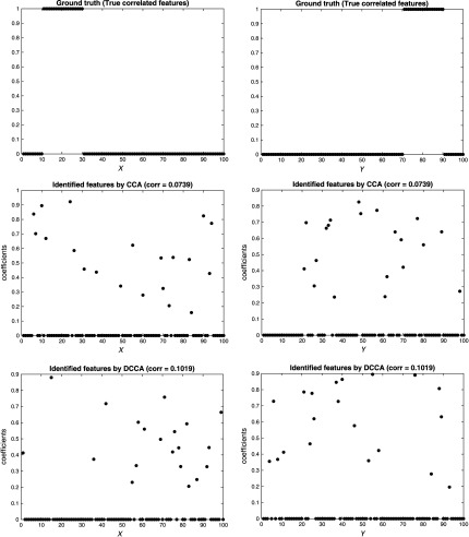
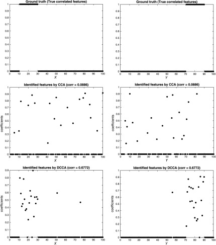
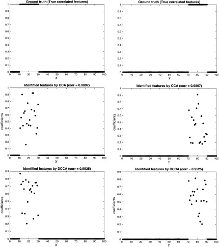
In each scenario, we implemented both CCA and our model, DCCA, to detect both correlation and true correlated features between two datasets. Note that loading vectors , were sparse vectors in our experiment setting, i.e., most of the elements were zeros. The numbers of features, i.e., , , were 100 in our setting, among which only 20 features were set as true correlated features. That is to say, the length of loading vectors and was 100, and only 20 of their elements were nonzeros, as shown at the top of Fig. 2. An ideal method should be able to accurately detect the cross-data correlation and also the 20 true correlated features.
Fig. 2.
Performance comparison between CCA and DCCA [independence scenario: Fig. 1(a)].
The results are shown in Figs. 2, 3, 4, for the three scenarios, respectively. In each figure, the top two subfigures represent the ground truth of the true correlated features, and the bottom four subfigures represent the identified features by CCA and DCCA, respectively. From Fig. 2, when two data are independent, both CCA and DCCA detect a weak correlation (CCA: 0.0739 versus DCCA: 0.1019) and neither method can identify true correlated features. From Fig. 4, when two data follow a linear relationship, both CCA and DCCA can detect a strong correlation (CCA: 0.9807 versus DCCA: 0.9525) and both methods can accurately identify the true correlated features. From Fig. 3, when two data follow a nonlinear relationship, CCA cannot detect the correlation (CCA: 0.0886) and cannot identify the true correlated features. In comparison, DCCA can detect the nonlinear correlation (DCCA: 0.6772) and also the true correlated features. The results in the three scenarios, i.e., Figs. 1–4, verified the superior performance of DCCA over conventional CCA in terms of detecting both complex correlations and true correlated features.
Fig. 3.
Performance comparison between CCA and DCCA [nonlinear dependence scenario: Fig. 1(b)].
Fig. 4.
Performance comparison between CCA and DCCA [linear dependence scenario: Fig. 1(c)].
4. Application to Brain Imaging Data
4.1. Brain Imaging Data and Brain Connectivity
The DCCA was then applied to a brain development study focused on two experiments. One experiment is to study the imaging-genetic associations (Sec. 4.3) and the other one is to study the connections between different brain subnetworks or subdomains, e.g., default mode network (DMN), and how the connections change across different age stages (Sec. 4.5). Imaging-genetic study analyzes the correlation between fMRI data, which detects the change of the brain functional activity at voxel level and SNPs data. SNPs are important genetic factors underlying differences in phenotypes among human beings. Genetic factors may function as a complicated group, e.g., protein–protein interaction network, gene pathway, when regulating a certain phenotype or disease. Similarly, neurons and brain regions also function and harmonize in a connected network when performing a specific brain function.10 Therefore, distance CCA, which seeks the optimal combinations of features with the strongest cross-data associations, might be superior in detecting group–group nonlinear associations between brain imaging scans and genetic factors.
4.2. Data Collection and Preprocessing
The Philadelphia Neurodevelopmental Cohort (PNC)15 is a large-scale collaborative study between the Brain Behavior Laboratory at the University of Pennsylvania and the Children’s Hospital of Philadelphia. The data include fMRI and SNPs data of adolescents aged from 8 to 21 years. The fMRI data were collected during a resting state from 857 subjects. After the collection of raw fMRI data, SPM1216 was used to conduct motion correction, spatial normalization, spatial smoothing with a 3×3-mm Gaussian kernel, and multiple regression to mitigate the influence of motion. Finally, 264 ROIs (containing 21,384 voxels) were extracted based on the power coordinates17 with a sphere radius parameter of 5 mm. SNPs data were collected from 7863 subjects based on four platforms, Illumina Human610Quadv1, HumanHap550v1, HumanHap550v3, and HumanOmniExpress. SNPs with missing values were deleted and the rest missing values were further imputed using Plink.18,19 Then, the SNPs within gene bodies were kept, resulting in 95,639 SNPs.
4.3. Imaging-Genetic Associations
In order to implement distance CCA, the subjects having both fMRI and SNP data are further extracted, resulting in 855 subjects. For fMRI data, the stimulus-on versus stimulus-off contrast was obtained from the raw resting-state time series data. To find the interactions that are more related to mental disorders, SNPs located in genes associated with brain disorders were kept, where the brain disorders included schizophrenia, bipolar disorder, depression, attention-deficit/hyperactivity disorder, and post-traumatic stress disorder. Finally, 736 genes containing 21,487 SNPs were left for further analysis.
When applied to detect the group associations between fMRI and SNPs, distance CCA identified a subset of 45 genes and a subset of 15 ROIs that were strongly correlated. The distance correlation between the identified ROIs and genes was 0.2047 with -value of (calculated based on Eq. 6). In comparison, the largest single ROI–gene distance correlation is 0.1759 with -value of . This demonstrated that distance covariance-based CCA can find a pair of variable groups with an enhanced distance correlation and significance level. The lists of the identified genes and ROIs are in Tables 1 and 2, respectively. The locations of the identified ROIs are further visualized in Fig. 5 using the BrainNet Viewer toolbox.14,20
Table 1.
The genes identified by DCCA.
| Gene | Gene | Gene | Gene | Gene |
|---|---|---|---|---|
| RERE | OPRD1 | FAF1 | MIR137HG | CADM3 |
| AKT3 | LOC101929452 | CYP26B1 | SLC4A5 | INPP4A |
| HAT1 | CIR1 | ZNF330 | CLCN3 | CTC-436P18.1 |
| LOC102467655 | MEF2C-AS1 | CDC25C | CAP2 | SP4 |
| FAM126A | ATP6V1B2 | BNIP3L | LETM2 | C8orf87 |
| NAPRT1 | NT5C2 | EIF3F | MARK2 | TRPT1 |
| ZNF202 | SIAE | NRGN | PAWR | C12orf76 |
| MAP3K9 | TRAF3 | CALB2 | YWHAE | SRR |
| PRRG2 | DNMT3B | ARHGAP40 | KCNS1 | YPEL1 |
Table 2.
The identified brain ROIs. , , represent ROI coordinates in the Montreal Neurological Institute (MNI) space.
| ROI name | Suggested system | |||
|---|---|---|---|---|
| 13 | 75 | Postcentral gyrus | Sensory/somatomotor hand | |
| 29 | 71 | Precentral gyrus | Sensory/somatomotor hand | |
| 44 | 57 | Precentral gyrus | Sensory/somatomotor hand | |
| 75 | Precentral gyrus | Sensory/somatomotor hand | ||
| 66 | 25 | Precentral gyrus | Sensory/somatomotor mouth | |
| 65 | 20 | Superior temporal gyrus | Auditory | |
| 13 | 55 | 38 | Superior frontal gyrus | Default mode |
| 55 | 39 | Superior frontal gyrus | Default mode | |
| 6 | 64 | 22 | Medial frontal gyrus | Default mode |
| 65 | Middle temporal gyrus | Default mode | ||
| 52 | 7 | Middle temporal gyrus | Default mode | |
| 18 | Parahippocampa gyrus | Visual | ||
| 20 | 2 | Lingual gyrus | Visual | |
| 26 | Lingual gyrus | Visual | ||
| 51 | 17 | Superior frontal gyrus | Salience |
Fig. 5.

The sagittal, coronal, and axial views of the identified brain ROIs. Figures were drawn using the BrainNet viewer toolbox.14
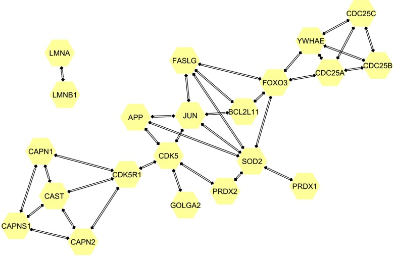
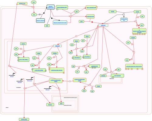
After that, gene enrichment analysis was conducted to reveal the underlying biological functions of the identified genes. Ten pathways were selected with a screening of -value (-value represents the multiple testing corrected -value), and the pathways together with their corresponding -values were listed in Table 3. -values are calculated using the hypergeometric test based on the numbers of genes in the particular biological pathway and the identified gene set. The -values are then calculated by correcting the -values using multiple testing correction, e.g., Bonferroni correction,8 based on the false discovery rate method. Among the identified pathways, pathways “neurodegenerative diseases,” “oxidative damage,” and “deregulated CDK5 triggers multiple neurodegenerative pathways in Alzheimer’s disease models” have been reported to be related to neuron activities and brain development. Pathway “neurodegenrative diseases” is related to the death of neurons and corticobasal degeneration, which might further lead to the progressive dysfunction in the brain and a number of mental disorders.21 Pathway “oxidative damage,” which is related to cell signaling, may lead to damage of cell and the death of neurons.22 It may be related to the pathogenesis of several neural degenerative diseases, including Parkinson’s disease,23 depression,24 and Alzheimer’s disease.25 For pathway “deregulated CDK5 triggers multiple neurodegenerative pathways in Alzheimer’s disease models,” abnormal CDK5 may result in unregulated activation of the cycle of cell,26 which might further lead to the death of neurons.27 Mental disorders, such as Alzheimer’s disease, may occur if CDK5 is deregulated.28 The interactions of pathway “neurodegenerative diseases” and “deregulated CDK5 triggers multiple neurodegenerative pathways in Alzheimer’s disease models” are visualized in Figs. 6 and 7, respectively. Figure 6 was plotted using Cytoscape software,29 which was an open source platform for visualizing complex networks. Figure 7 was generated using reactome pathway database.30
Table 3.
Gene enrichment analysis of the identified genes. -values represent multiple testing corrected -value.
| Pathway name | Source | -value | -value |
|---|---|---|---|
| Chk1/Chk2(Cds1)-mediated inactivation of cyclin B:Cdk1 | Reactome | 0.00032 | 0.012 |
| Activation of BAD and translocation to mitochondria | Reactome | 0.00044 | 0.013 |
| Deregulated CDK5 triggers multiple neurodegenerative | Reactome | 0.00063 | 0.013 |
| Pathways in Alzheimer’s disease models | |||
| Neurodegenerative diseases | Reactome | 0.00063 | 0.013 |
| TNFalpha | NetPath | 0.0013 | 0.021 |
| Activation of BH3-only proteins | Reactome | 0.0018 | 0.023 |
| Class I PI3K signaling events mediated by Akt | PID | 0.0024 | 0.027 |
| Oxidative damage | Wikipathways | 0.0031 | 0.029 |
| LKB1 signaling events | PID | 0.0036 | 0.029 |
| Intrinsic pathway for apoptosis | Reactome | 0.0036 | 0.029 |
Fig. 6.
The interaction mechanisms of the pathway “neurodegenerative diseases.”
Fig. 7.
The interaction mechanisms of the pathway “deregulated CDK5 triggers multiple neurodegenerative pathways in Alzheimer’s disease models.”
For brain imaging data, as shown in Table 2, the majority (13/15) of the detected ROIs are from three brain subdomains: sensorimotor network (SM), DMN, and visual network (VIS). SM is related to the coordination of the body when performing motor tasks.31 DMN is the dominant network when subjects are in resting state, mind-wandering, or not involved in a specific task. Dysfunction within the DMN has been associated with several mental disorders,32,33 e.g., schizophrenia, depression, autism, etc. Associations between DMN and genetic factors exist according to a multivariate study of schizophrenia subjects scanned during the resting state.34
4.4. Functional Connectivity Between Brain Subnetworks
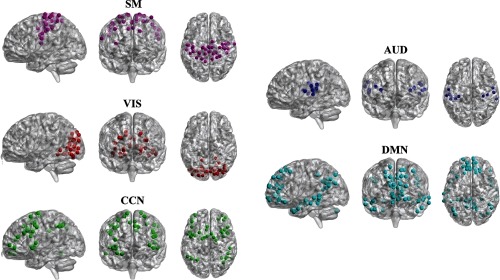
For brain FC study, we selected five brain subnetworks or subdomains and then applied distance CCA to investigate the connections between each subnetwork pair and to study the age effects on the connections. Resting-state fMRI was used in this experiment and data were preprocessed using group ICA of fMRI toolbox35 for independent component analysis (ICA).36 The five brain subnetworks include SM, VIS, cognitive control network (CCN), auditory network (AUD), and DMN, and the corresponding locations in the brain are shown in Fig. 8.
Fig. 8.
The sagittal, coronal, and axial views of brain functional network domains extracted via group ICA. The names of the brain network domains are: SM, AUD, VIS, DMN, CCN, and salience network (SAL).
In order to investigate both linear and nonlinear connections of the brain, we applied both linear CCA and distance CCA to the PNC data and the results are shown in Fig. 9. The results were based on a 10-fold cross-validation, in which each time five folds were used as training data and the rest five folds were used as testing data. It is noteworthy that the metric of distance correlation is different from that of linear Pearson correlation, e.g., distance correlation Pearson correlation . Nevertheless, distance correlation reflects the relative strength of the dependence between two variables. From Fig. 9, strong linear connections are detected between each pair of SM, VIS, CCN, and AUD networks, while the linear connections between DMN and other networks are weak. Research32 has shown that DMN may have strong intrinsic connections while the connections between DMN and the rest networks are weak in the resting state, which is consistent with the result of linear CCA. In comparison, distance CCA detected stronger DMN-SM, DMN-CCN, and DMN-AUD connections, which might be a new discovery.
Fig. 9.
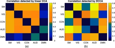
The heatmap showing the correlations between brain networks. (a) The results by linear CCA and (b) the results by DCCA. The color bar indicates the value of detected correlations.
4.5. Ages Effects on Brain FC
It is of interest to investigate how brain connectivity changes during adolescence and how it changes across different age stages, e.g., children and young adults, which may further contribute to the study of normal and pathological brain development. Three age groups, 8 to 11 years, 13 to 16 years, and 18 to 22 years, were selected and then distance CCA was applied to each age group to analyze brain network connections. Subjects aged 12 and 17 years were not included in the experiments in order to get a clear boundary between different age groups. The connections between brain subnetworks for each age group are shown in Fig. 10. From Fig. 10, the patterns of the connections are different between different age groups. For instance, the connections between different brain networks are relatively weaker at age 8 to 11 but become relatively stronger at age 13 to 16 and age 18 to 22. It demonstrates that different brain regions become more and more connected during adolescence, which may be a result of the training and development of the brain during multiple types of brain activities. Moreover, it seems that the connections between CCN and SM are weak across all three age groups, which indicates that the connection between CCN and SM may be weak at the adolescent stage.
Fig. 10.
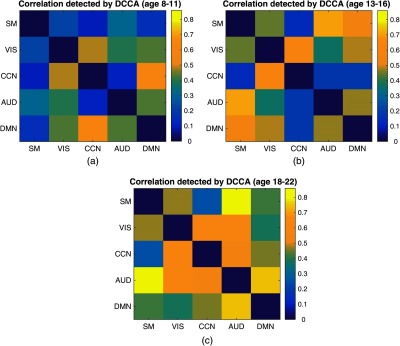
The heatmap showing age differences in brain connectivity links in resting state. (a) The network connection for age group 8 to 11 years; (b) the network connection for age group 13 to 16 years; and (c) the network connection for age group 18 to 22 years. The color bar indicates the value of detected correlations.
5. Discussion and Conclusion
In this work, we proposed a new model, DCCA, which overcomes the limitation of distance correlation in detecting significant associations when feature size is large. Conventional distance correlation analysis needs large-scale multiple testing when testing feature–feature association simultaneously. The proposed model, DCCA, addresses the problem by searching a combination of original features with the highest distance correlation. It is achieved by first constructing a distance kernel function and then solving an optimization problem. The ability to detect nonlinear group–group associations makes DCCA more suitable for analyzing complex multi-omics and imaging-genetic associations, in which both genetic factors and brain ROIs may work as groups when regulating a phenotype or performing a specific brain function.
When applied to imaging-genetic association study, DCCA detected a strong correlation between a subset of genes and a subset of brain ROIs with an improved significance level. Several neuron degeneration and mental disorder related pathways were enriched from the identified genes after gene enrichment analysis, which demonstrated the biological significance of our findings. In addition, DCCA found several mental disorder-related brain networks which had been reported by existing literature. Experiments on brain connectivity study also found several new discoveries using DCCA. Brain network DMN, which is considered to be distinct from other brain domains/networks, may have strong nonlinear connections with other brain networks according to the results of DCCA. When applied to analyzing each age groups, DCCA reveals that younger groups (8 to 11 years) exhibit weak connections of brain networks while the connections become strong at an older age stage (13 to 16 and 18 to 22) which may a result of brain development. The discoveries of imaging genetic associations and brain connections verified the performance of DCCA. Besides the examples in this study, it may find more applications in multiimaging and multi-omics studies, where identifying correlations between multiple datasets is a common challenge.
Acknowledgments
The authors would like to thank the NIH (P30 GM122734, R01 GM109068, R01 MH104680, R01 MH107354, P20 GM103472, R01 REB020407, and R01 EB006841) and NSF (#1539067) for partial support.
Biographies
Wenxing Hu received his BS degree in applied mathematics from Xi’an Jiaotong University, China, 2011. Now, he is a PhD student in biomedical engineering, Tulane University, USA. His research interests include machine learning and deep learning, dimension reduction, correlation analysis, and multi-omics data integration.
Aiying Zhang received her BS degree in statistics from the University of Science and Technology of China. She is now a PhD student in the Department of Biomedical Engineering, Tulane University. Her research interests mainly focus on graphical models (directed and undirected) with applications in multi-omics data integration.
Biao Cai received his BS and MS degrees in biomedical engineering from Tianjin University, China, in 2013 and 2016, respectively. Now, he is a PhD student in biomedical engineering, Tulane University, USA. His research interests include dictionary learning and time-varying graphical LASSO, dynamic function network connectivity, and brain development.
Vince Calhoun is currently president for the MRN, and a distinguished professor in the ECE Department, University of New Mexico. He has published over 600 journal articles. His work includes ICA-based fMRI analysis, and data fusion of multimodal-imaging and genetics data. He leads an NIH P20 COBRE grant on multimodal imaging of mental disorders and an NSF EPSCoR grant focused on brain imaging and epigenetics of adolescent development. He is a fellow of the American Association for the Advancement of Science, the American Institute of Biomedical and Medical Engineers, the American College of Neuropsychopharmacology, and the International Society of Magnetic Resonance in Medicine.
Yu-Ping Wang received his BS degree from Tianjin University in 1990, and his MS and PhD degrees from Xian Jiaotong University in 1993 and 1996, respectively. He is currently a professor of biomedical engineering at Tulane University. His research interests include computer vision, signal processing, and machine learning with applications to biomedical imaging and bioinformatics, where he has published about 200 publications. He has served on numerous NSF/NIH review panels, and as editor for several journals.
Disclosures
The authors have no relevant financial interests in the paper and no other potential conflicts of interest to disclose.
References
- 1.Hotelling H., “Relations between two sets of variates,” Biometrika 28(3/4), 321–377 (1936). 10.2307/2333955 [DOI] [Google Scholar]
- 2.Fang J., et al. , “Joint sparse canonical correlation analysis for detecting differential imaging genetics modules,” Bioinformatics 32(22), 3480–3488 (2016). 10.1093/bioinformatics/btw485 [DOI] [PMC free article] [PubMed] [Google Scholar]
- 3.Hlinka J., et al. , “Functional connectivity in resting-state fMRI: is linear correlation sufficient?” Neuroimage 54(3), 2218–2225 (2011). 10.1016/j.neuroimage.2010.08.042 [DOI] [PMC free article] [PubMed] [Google Scholar]
- 4.Székely G. J., et al. , “Measuring and testing dependence by correlation of distances,” Ann. Stat. 35(6), 2769–2794 (2007). 10.1214/009053607000000505 [DOI] [Google Scholar]
- 5.Geerligs L., et al. , “Functional connectivity and structural covariance between regions of interest can be measured more accurately using multivariate distance correlation,” NeuroImage 135, 16–31 (2016). 10.1016/j.neuroimage.2016.04.047 [DOI] [PMC free article] [PubMed] [Google Scholar]
- 6.Fang J., et al. , “Fast and accurate detection of complex imaging genetics associations based on greedy projected distance correlation,” IEEE Trans. Med. Imaging 37(4), 860–870 (2018). 10.1109/TMI.2017.2783244 [DOI] [PMC free article] [PubMed] [Google Scholar]
- 7.Székely G. J., Rizzo M. L., “The distance correlation t-test of independence in high dimension,” J. Multivar. Anal. 117, 193–213 (2013). 10.1016/j.jmva.2013.02.012 [DOI] [Google Scholar]
- 8.Holm S., “A simple sequentially rejective multiple test procedure,” Scand. J. Stat. 6(2), 65–70 (1979). [Google Scholar]
- 9.Hu W., et al. , “A hybrid correlation analysis with application to imaging genetics,” Proc. SPIE 10579, 1057905 (2018). 10.1117/12.2293556 [DOI] [Google Scholar]
- 10.Rubinov M., Sporns O., “Complex network measures of brain connectivity: uses and interpretations,” Neuroimage 52(3), 1059–1069 (2010). 10.1016/j.neuroimage.2009.10.003 [DOI] [PubMed] [Google Scholar]
- 11.Jöreskog K. G., Goldberger A. S., “Estimation of a model with multiple indicators and multiple causes of a single latent variable,” J. Am. Stat. Assoc. 70(351a), 631–639 (1975). 10.1080/01621459.1975.10482485 [DOI] [Google Scholar]
- 12.Parkhomenko E., Tritchler D., Beyene J., “Sparse canonical correlation analysis with application to genomic data integration,” Stat. Appl. Genet. Mol. Biol. 8(1), 1–34 (2009). 10.2202/1544-6115.1406 [DOI] [PubMed] [Google Scholar]
- 13.Lin D., Calhoun V. D., Wang Y.-P., “Correspondence between fmri and SNP data by group sparse canonical correlation analysis,” Med. Image Anal. 18(6), 891–902 (2014). 10.1016/j.media.2013.10.010 [DOI] [PMC free article] [PubMed] [Google Scholar]
- 14.Xia M., Wang J., He Y., “BrainNet Viewer: a network visualization tool for human brain connectomics,” PloS ONE 8(7), e68910 (2013). 10.1371/journal.pone.0068910 [DOI] [PMC free article] [PubMed] [Google Scholar]
- 15.Satterthwaite T. D., et al. , “Neuroimaging of the Philadelphia NeuroDevelopmental Cohort,” Neuroimage 86, 544–553 (2014). 10.1016/j.neuroimage.2013.07.064 [DOI] [PMC free article] [PubMed] [Google Scholar]
- 16.Friston K., et al. , “Statistical parametric mapping,” http://www.fil.ion.ucl.ac.uk/spm/software/spm12/ (25 September 2018).
- 17.Power J. D., et al. , “Functional network organization of the human brain,” Neuron 72(4), 665–678 (2011). 10.1016/j.neuron.2011.09.006 [DOI] [PMC free article] [PubMed] [Google Scholar]
- 18.Chang C., et al. , “PLINK,” https://www.cog-genomics.org/plink/2.0/ (1 April 2019).
- 19.Purcell S., et al. , “PLINK: a tool set for whole-genome association and population-based linkage analyses,” Am. J. Human Genet. 81(3), 559–575 (2007). 10.1086/519795 [DOI] [PMC free article] [PubMed] [Google Scholar]
- 20.Xia M., et al. , “BrainNet Viewer,” https://www.nitrc.org/projects/bnv/ (7 July 2011).
- 21.Seeley W. W., et al. , “Neurodegenerative diseases target large-scale human brain networks,” Neuron 62(1), 42–52 (2009). 10.1016/j.neuron.2009.03.024 [DOI] [PMC free article] [PubMed] [Google Scholar]
- 22.Evans M. D., Cooke M. S., “Factors contributing to the outcome of oxidative damage to nucleic acids,” Bioessays 26(5), 533–542 (2004). 10.1002/bies.20027 [DOI] [PubMed] [Google Scholar]
- 23.Hwang O., “Role of oxidative stress in Parkinson’s disease,” Exp. Neurobiol. 22(1), 11–17 (2013). 10.5607/en.2013.22.1.11 [DOI] [PMC free article] [PubMed] [Google Scholar]
- 24.Jiménez-Fernández S., et al. , “Oxidative stress and antioxidant parameters in patients with major depressive disorder compared to healthy controls before and after antidepressant treatment: results from a meta-analysis,” J. Clin. Psychiatry 76, 1658–1667 (2015). 10.4088/JCP.14r09179 [DOI] [PubMed] [Google Scholar]
- 25.Valko M., et al. , “Free radicals and antioxidants in normal physiological functions and human disease,” Int. J. Biochem. Cell Biol. 39(1), 44–84 (2007). 10.1016/j.biocel.2006.07.001 [DOI] [PubMed] [Google Scholar]
- 26.Lopes J., Oliveira C., Agostinho P., “Cell cycle re-entry in Alzheimer’s disease: a major neuropathological characteristic?” Curr. Alzheimer Res. 6(3), 205–212 (2009). 10.2174/156720509788486590 [DOI] [PubMed] [Google Scholar]
- 27.Chang K.-H., Vincent F., Shah K., “Deregulated cdk5 triggers aberrant activation of cell cycle kinases and phosphatases inducing neuronal death,” J. Cell Sci. 125(21), 5124–5137 (2012). 10.1242/jcs.108183 [DOI] [PubMed] [Google Scholar]
- 28.Yang Y., Mufson E. J., Herrup K., “Neuronal cell death is preceded by cell cycle events at all stages of Alzheimer’s disease,” J. Neurosci. 23(7), 2557–2563 (2003). 10.1523/JNEUROSCI.23-07-02557.2003 [DOI] [PMC free article] [PubMed] [Google Scholar]
- 29.Shannon P., et al. , “Cytoscape: a software environment for integrated models of biomolecular interaction networks,” Genome Res. 13(11), 2498–2504 (2003). 10.1101/gr.1239303 [DOI] [PMC free article] [PubMed] [Google Scholar]
- 30.Croft D., et al. , “The reactome pathway knowledgebase,” Nucleic Acids Res. 42(D1), D472–D477 (2013). 10.1093/nar/gkt1102 [DOI] [PMC free article] [PubMed] [Google Scholar]
- 31.Chenji S., et al. , “Investigating default mode and sensorimotor network connectivity in amyotrophic lateral sclerosis,” PLoS ONE 11(6), e0157443 (2016). 10.1371/journal.pone.0157443 [DOI] [PMC free article] [PubMed] [Google Scholar]
- 32.Buckner R. L., Andrews-Hanna J. R., Schacter D. L., “The brain’s default network,” Ann. New York Acad. Sci. 1124(1), 1–38 (2008). 10.1196/annals.1440.011 [DOI] [PubMed] [Google Scholar]
- 33.Akiki T. J., et al. , “Default mode network abnormalities in posttraumatic stress disorder: a novel network-restricted topology approach,” NeuroImage 176, 489–498 (2018). 10.1016/j.neuroimage.2018.05.005 [DOI] [PMC free article] [PubMed] [Google Scholar]
- 34.Meda S. A., et al. , “Multivariate analysis reveals genetic associations of the resting default mode network in psychotic bipolar disorder and schizophrenia,” Proc. Natl. Acad. Sci. U. S. A. 111(19), E2066–E2075 (2014). 10.1073/pnas.1313093111 [DOI] [PMC free article] [PubMed] [Google Scholar]
- 35.Calhoun V. D., et al. , “Group ICA of fMRI Toolbox (GIFT),” http://mialab.mrn.org/software/gift/ (20 Feburary 2017).
- 36.Calhoun V. D., Adali T., “Multisubject independent component analysis of fMRI: a decade of intrinsic networks, default mode, and neurodiagnostic discovery,” IEEE Rev. Biomed. Eng. 5, 60–73 (2012). 10.1109/RBME.2012.2211076 [DOI] [PMC free article] [PubMed] [Google Scholar]


