Currently available bulk sequencing data does not necessarily support a model of neutral tumor evolution

In a recent contribution¹, Williams et al. used next-generation sequencing data of tumor bulk samples to derive their hypothesis that selection is limited to times before malignant transformation while tumor cell populations afterwards evolve exclusively by neutral evolution. The authors arrived at their conclusions by showing that the expected number of mutations (M) in an exponentially increasing population undergoing only neutral evolution grows linearly with the inverse allele frequency (1/f) of mutant alleles. The allele frequency of a variant is defined as the proportion of cells containing that particular variant. Their reasoning was based on the fact that in a neutrally evolving cell population, all subclones grow at the same rate, so the allele frequency is fixed as the inverse of the number of cells present at the time of appearance of a new variant. The authors then concluded that a tumor displaying a linear relationship between the number of mutations and the inverse allele frequency should imply that the population evolves without selection. They also performed simulations of a branching process model with selection to show that selection cannot explain a linear relationship between M and 1/f. Furthermore, they observed a high correlation between M and 1/f in about one third of patient samples investigated, as further indication of neutral tumor evolution. Their findings corroborate previous results² based on the ‘Big Bang’ model that suggested a similar conclusion in colorectal cancer using single time point bulk sequencing data.

We believe that the authors arrived at an erroneous conclusion, which also stands in contrast to most other recent findings^3,4,5 in this field, based on flawed logic known as the ‘fallacy of the converse’. The fact that a model of neutral evolution leads to a linear relationship between M and 1/f does not imply that a linear relationship proves the presence of neutral evolution. In more abstract terms, A implying B does not necessarily mean that B implies A. Here we demonstrate that models with selection can also lead to a linear relationship between M and 1/f, and that, therefore, linearity is a bad test statistic and cannot be used to distinguish between populations evolving with and without selection. Our results unequivocally demonstrate that the claims made by Williams et al. have little merit.

To demonstrate this fact, we here designed and analyzed two alternative stochastic evolutionary models that both return a linear relationship and show similarly high $R^2$ values for neutral as well as selection scenarios. To be consistent with the assumptions of the model and results used by Williams et al¹, both models are based on exponentially growing non-competing cellular populations with no spatial or micro-environmental effects and thus represent, by design, simplified versions of the tumorigenic process. The first model is a simple birth-death process of mutation accumulation (Fig. 1). In this model, each new mutation event gives rise to a single variant allele. This approach allows derivation of exact expressions for the expected size of all mutant clones, thus providing an easy way of testing the authors’ claim that a linear relationship can arise only from neutrality. The second model is a more complex infinite-allele branching process model (Fig. 2) where multiple mutations may arise and lead to unique clones, making it analogous to the model developed by the authors. In both models, additive fitness effects in new clones are chosen from a fitness distribution so that any new mutant has a different birth rate that can lead to faster (or slower) growth compared to the parent clone. Furthermore, the second model incorporates more complex assumptions such as the infinite-allele model (rendering all mutants unique) as well as cell sampling and a Poisson-distributed number of variants (see below for details) to more closely match the model analyzed previously1. Simulation results from both models demonstrate unequivocally that neutral (i.e. drift only) and selective evolution both give rise to linear relationships between M and 1/f. Using both models, we tested a number of scenarios of selection, including intentionally chosen extreme (though biologically improbable) cases where every clone has a large fitness advantage/disadvantage. Even under such selection scenarios we demonstrate that linearity with high R² values arise, highlighting the serious flaw in the authors’ method of determining neutral evolution from curves with high R² values.

Figure 1. A simple branching process model of tumor evolution.

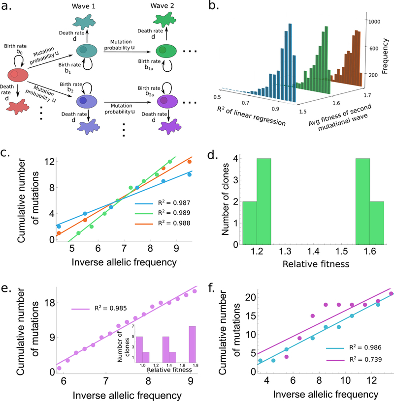
(a.) Schematic representation for the accumulation of mutations in our model. (b.) Histogram of R² values for the model with two mutational waves. Fitness values are as follows: type-0 : 0.9, type-i : 1+N(0.2, 0.012), type-ia : 1+N($\mu ,0.012)$ with $\mu =0.5$ (blue), 0.6 (green), 0.7 (orange). Histograms are generated from 5000 draws from N($\mu ,\sigma$). (c.) One example draw with R² > 0.985 from each of the three cases in (b.) are shown with corresponding color codes. (d.) Fitness distribution of the clones corresponding to $\mu =0.6$ (corresponding to green in (b.) and (c.)). (e.),(f.) Same as (c.),(d.) but with three waves of mutations. Fitness values in (f.) were chosen from a log-normal distribution with same parameters as (e.). The total size of the tumor in all cases is allowed to reach anywhere between 6×10⁷ to 7×10¹¹ cells.

Figure 2. An infinite-allele branching process model of tumor evolution, including sampling as in in Williams et al.¹.

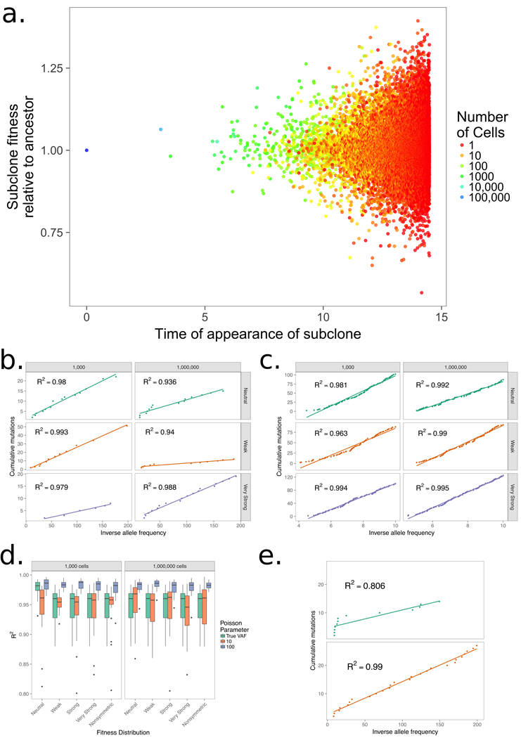
We initiate each process with a single ancestor with birth rate of 1, a death rate of 0.1, and a double exponential fitness distribution with mean fitness change of 0.01 (weak), 0.04 (strong), and 1 (very strong) along with a neutral evolution model where there is no change in fitness and a model with only increasing fitness changes. (a.), The panel shows the time of a new subclone’s appearance with the birth rate colored by the subclone’s size at the end of the simulation, showing that the subclone size in a simulation with strong selection is associated with age, but also with its fitness. Allowing the simulation to run longer would result in younger subclones with high fitness outcompeting older ones. (b.) A plot of the cumulative number of mutations (M) and inverse allele frequency (1/f) shows linear trends in simulations where a single mutation arises from any mutation event and no additional noise is added to mimic the effect of sequencing. (c.) A linear trend is apparent between M and 1/f in the same model where each new mutation event contains Poisson(100) mutations and alleles are sampled to account for sequencing errors to create a result that follows the methods of Williams et al.¹ (d.) Boxplots for 25 simulation in all models for 1,000 and 1,000,000 cells show there is little change in R² as selection becomes larger, but allowing multiple mutations to occur at any mutation event has a large effect on linearity. (e.) The model is able to recapitulate nonlinear curves suggesting the models with selection do not necessarily result in linear curves, but can result in both types.

In the first model (Fig. 1a), clonal expansion begins with a single cell of the original, tumor-initiating type (type-0), which proliferates and dies with rates $b_0$ and d, respectively, and may accumulate mutations with probability u during each cell division. The resulting mutant cells of type-$i(i>0$, birth rate b_i and death rate d) constitute the first wave of mutated cells which in turn can mutate to produce the second wave (type-$ia$, birth-rate $b_{ia}$ and death rate d), and so on. By deriving the differential equations governing the time-evolution of this model, the expected number of cells of any type can be exactly solved for over time (see ⁶ for details of the solution). We first explored the case of two mutational waves (Fig. 1c,d). The additive fitness values (additional birth rates) of the cell types are chosen from a normal distribution $N(\mu , \sigma )$ with mean $\mu$ and standard deviation $\sigma .$ We allowed $\mu$ to become progressively larger with the wave number. The cumulative frequencies of cell types ($M$) were then calculated as a function of inverse frequency ($1/f$), and the $R^2$ of linear regression between $M$ and $1/f$ are calculated (examples where $R^2>0.985$ are shown in Fig. 1c). This process was performed 5,000 times, and histograms were generated showing the distribution of $R^2$ values (Fig. 1b). This simple model of mutation accumulation already demonstrates that linear curves with high $R^2$ values can be easily obtained even when mutant cells are allowed to have large (~50–80%) fitness advantages. This model is limited by the number of distinct clones present, which results in only a few data points for the linearity test (Fig. 1c). To check whether increasing the number of clones affects our results, we allowed for the possibility of a third mutational wave (Fig. 1e,f), which significantly increases the number of data points based on which R² is calculated. We also tested the ability of asymmetric fitness distributions to produce high R² values by choosing the additive fitness of mutants from a log-normal distribution with same parameters as the previously used normal distribution (Fig. 1f). In all cases, R² values greater than 0.98 are easily obtained, thereby confirming our claim that models with selection can generate linear $M$ vs $1/f$ curves. Finally, we also show a curve where the R² metric is less than 0.98 (in Fig. 1f). The non-linearity seen in this example is qualitatively similar to the examples shown by the authors in their Supplementary Figure 11, thereby proving that this oversimplified model does recapitulate all scenarios demonstrated originally by the authors.

To go beyond this simplest model, we then constructed a continuous-time birth-death-mutation process analogous to the model created in 1. Our process allows cells to live for an exponentially distributed time before dividing or dying, and cells may accumulate mutations during each cell division according to a given probability distribution (for details of the simulation technique, see ⁷). To match the approach in 1, a new mutant cell contains a Poisson-distributed number of variants with rate 100, which is the same distribution and rate chosen by the authors. This approach allows multiple variants to arise at each mutation event, and sampling to account for sequencing noise results in multiple alleles with similar, but not identical, frequencies. Under the neutral model, mutant cells have the same birth rate as their parents, but when allowing for selection, a mutant cell has a birth rate equal to the sum of a parent’s rate and an additional fitness term generated from a double exponential distribution, allowing mutations to be deleterious or advantageous. We continue the process until 1,000 cells (as in 1) and 1,000,000 cells to demonstrate how time, in addition to selection, affects linearity between M and 1/f. The ancestor individual splits into two new cells with rate b=1 and dies with rate d=0.1. Given a split, one of the daughter cells may become a mutant with probability μ, which is 0.1 for the 1,000 cell scenario and 0.03 for the 1,000,000 cell scenario. A mutation results in a new clone with a birth rate of b + s, where s is chosen from the fitness distribution. We consider multiple levels of selection and a model with only advantageous selection. These levels of selection based on the width of the fitness distribution, parameterized by the rate of the exponential distribution. Weak selection is associated with a rate parameter of 100 for the double exponential fitness distribution, leading to an average change in the birth rate of 0.01 for a single mutation, while strong selection has a wider fitness distribution with a rate parameter of 25 that changes the fitness by an average of 0.04. Very strong selection is also included where the rate parameter is 1 so that the fitness doubles or halves on average with each new clone, representing a very extreme and significant increase. Finally, the asymmetric distribution is a one-sided exponential distribution with a rate of 25 where fitness only increases in the population. As mutations accumulate, the fitness of subclones increases as well, and the stronger selection scenarios are expected to lead to many more subclones with large fitness values relative to the ancestor fitness.

The results of our more complex model (Fig. 2) indicate that the contribution of clones to the final total population size is mainly due to early mutations, but the accumulating fitness suggests that later subclones have the ability to outcompete previous ones given enough time. Later subclones with large fitness values are still small due to their young age, but will eventually outcompete older, less fit clones. These subclones have usually accumulated multiple mutations, which allow for larger fitness values. The overlap in sizes among clones (Fig. 2a) also indicates that we cannot use cell counts or allele frequencies as a surrogate for time or age in such a population. Limiting our analysis to allele frequencies of [0.12, 0.24] as in 1, the true allele frequency without accounting for multiple mutations or sequencing error is noticeable (Fig. 2b), but this effect is much stronger when multiple mutations are allowed to occur in an individual event and alleles are sampled from the population to represent noise to obtain results similar to the original analysis (Fig. 2c). Changing the Poisson parameter has the largest effect on linearity as indicated by the boxplots, and there is no apparent effect due to the strength of selection in the model (Fig 2d). This observation suggests that $R^2$, or even linearity, is not a proper statistic to distinguish neutral from selection regimes, since either regime tends toward a linear relationship.

Even more impressive is the drastic increase in $R^2$ as we increase the final cell count (Fig. 2b,c). The cumulative number of mutations for an individual sample in each scenario increases linearly with respect to inverse allele frequency in all scenarios and the conformation to linearity becomes much stronger as the population size increases. However, we also show examples of a relatively high $R^2$ at 1,000 cells that have nonlinear relationships. This fact illustrates the danger in using R² as a cutoff point, especially at such a high value where minor differences changes the conclusion between neutral or selective evolution. Thus, we show relatively broad scenarios of evolution with selection that fit the original model1. This observation suggests that convergence to a linear relationship between mutation count and allele frequency is shared among branching process models under the infinite-allele assumption, as previously shown^8,9, suggesting that linearity may be achieved in even more general scenarios evolving according to branching processes.

However, linearity is not necessarily guaranteed for models with selection. The authors created a model with selection that leads to nonlinear trends between M and 1/f, as we were also able to do with our model (Fig. 2e). Using the code provided in 1, we found nonlinear trends for some simulation runs (Fig. 3a,b), but linear trends for others (Fig.3c-e). In fact, 5,000 simulations using their model with selection generates a distribution where a majority of simulations (66%) have R² values greater than 0.98 (Fig. 3f), proving that even their own code does not support the authors’ conclusion.

Figure 3. The model from Williams et al. for multiple simulations¹.

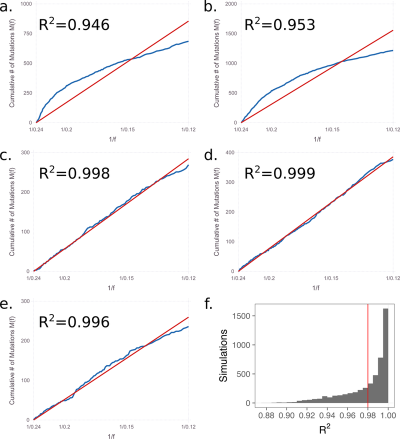
Using the code provided by Williams et al. for situations with selection, we show that linearity between the cumulative mutation count and inverse allele frequency is widespread. We used the code with different seed values than provided by the authors to initiate the random number generator. (a.) seed = 5 (provided); (b.) seed = 7 (provided); (c.) seed = 2; (d.) seed = 911; (e.) seed = 1234. (f.) a histogram of the R² for 5,000 runs of the code.

Our results demonstrate the difficulty in drawing conclusions about parameters in population kinetics based on data obtained at a single time point per patient. Even in the most simplified scenarios such as the absence of density-dependent interactions among cells and spatial components, the growth rate, mutation rate, and tumor/clone age are all unknowns and provide too many degrees of freedom to elucidate estimates from single time point data. Our findings serve to demonstrate that there is no way of differentiating neutral from selective evolution given the data used in 1 without obtaining additional quantitative molecular information about the tumor. In this context, one might be tempted to brandish Occam’s razor and choose an apparently simpler neutral model for the 30% of cases where a linear relation between M and 1/f was observed¹. However, since 70% of the data shows evidence of selection, a mixture model would then be required to account for all cases. This observation implies that choosing a neutral model to describe 30% of the data due to parsimony is disingenuous — a more complex model would inevitably be needed to describe all data. Considering that we are able to account for linearity and nonlinearity in a single model, our approach could therefore be considered more parsimonious.

Finally, there is grave danger in using an arbitrary $R^2$ value as a cutoff for linearity, especially when simulating branching processes to a number as low as 1,000 cells. We provided simulation results for neutral and selective evolution that provide similar results, yet within multiple simulation runs we observed a large amount of variability between sampled alleles. Increasing the final population size helps resolve that variability in both scenarios, further demonstrating the danger of using $R^2$ without other analysis or exploratory work and suggesting a trend toward linearity as the number of cells increases regardless of the type of process. Given the inability to conclude that neutral evolution necessarily underlies the observed tumor mutation frequencies, estimates of patient-specific in vivo mutation rates, contrary to the authors’ claims, are also scientifically inaccurate.

References

- 1.Williams Marc J., et al. “Identification of neutral tumor evolution across cancer types.” Nature genetics 48 (2016): 238–244. [DOI] [PMC free article] [PubMed] [Google Scholar]
- 2.Sottoriva Andrea, et al. “A Big Bang model of human colorectal tumor growth.” Nature genetics 47.3 (2015): 209–216. [DOI] [PMC free article] [PubMed] [Google Scholar]
- 3.Gerlinger Marco, et al. “Intratumor heterogeneity and branched evolution revealed by multiregion sequencing.” New England Journal of Medicine 366 (2012): 883–892. [DOI] [PMC free article] [PubMed] [Google Scholar]
- 4.Ding Li, et al. “Clonal evolution in relapsed acute myeloid leukaemia revealed by whole-genome sequencing.” Nature 481 (2012):506–510. [DOI] [PMC free article] [PubMed] [Google Scholar]
- 5.Welch John S., et al. “The origin and evolution of mutations in acute myeloid leukemia.” Cell 150 (2012): 264–278. [DOI] [PMC free article] [PubMed] [Google Scholar]
- 6.Chakrabarti Shaon, and Michor Franziska. “Pharmacokinetics and drug interactions determine optimum combination strategies in computational models of cancer evolution.” Cancer Research 77 (2017): 3908–3921. [DOI] [PMC free article] [PubMed] [Google Scholar]
- 7.McDonald Thomas O., and Michor Franziska. “SIApopr: A computational method to simulate evolutionary branching trees for analysis of tumor clonal evolution.” Bioinformatics 33, 2221–2223. [DOI] [PMC free article] [PubMed] [Google Scholar]
- 8.McDonald Thomas O., and Kimmel Marek. “A multitype infinite-allele branching process with applications to cancer evolution.” Journal of Applied Probability 52.3 (2015): 864–876. [Google Scholar]
- 9.Jagers Peter, and Nerman Olle. “The growth and composition of branching populations.” Advances in Applied Probability (1984): 221–259. [Google Scholar]