Structural variation and fusion detection using targeted sequencing data from circulating cell free DNA

Abstract

Motivation

Cancer is a complex disease that involves rapidly evolving cells, often forming multiple distinct clones. In order to effectively understand progression of a patient-specific tumor, one needs to comprehensively sample tumor DNA at multiple time points, ideally obtained through inexpensive and minimally invasive techniques. Current sequencing technologies make the ‘liquid biopsy’ possible, which involves sampling a patient’s blood or urine and sequencing the circulating cell free DNA (cfDNA). A certain percentage of this DNA originates from the tumor, known as circulating tumor DNA (ctDNA). The ratio of ctDNA may be extremely low in the sample, and the ctDNA may originate from multiple tumors or clones. These factors present unique challenges for applying existing tools and workflows to the analysis of ctDNA, especially in the detection of structural variations which rely on sufficient read coverage to be detectable.

Results

Here we introduce SViCT , a structural variation (SV) detection tool designed to handle the challenges associated with cfDNA analysis. SViCT can detect breakpoints and sequences of various structural variations including deletions, insertions, inversions, duplications and translocations. SViCT extracts discordant read pairs, one-end anchors and soft-clipped/split reads, assembles them into contigs, and re-maps contig intervals to a reference genome using an efficient k-mer indexing approach. The intervals are then joined using a combination of graph and greedy algorithms to identify specific structural variant signatures. We assessed the performance of SViCT and compared it to state-of-the-art tools using simulated cfDNA datasets with properties matching those of real cfDNA samples. The positive predictive value and sensitivity of our tool was superior to all the tested tools and reasonable performance was maintained down to the lowest dilution of 0.01% tumor DNA in simulated datasets. Additionally, SViCT was able to detect all known SVs in two real cfDNA reference datasets (at 0.6–5% ctDNA) and predict a novel structural variant in a prostate cancer cohort.

Availability

SViCT is available at https://github.com/vpc-ccg/svict. Contact:faraz.hach@ubc.ca

INTRODUCTION

A current challenge in precision oncology is the ability to track the progress of tumor in the patients; e.g. response to treatment. The classical approach for this would be to conduct tissue biopsies at different time points. This is an expensive and time consuming process, and since this in an invasive procedure, it may be difficult for the patient. Furthermore, if the tumor has undergone metastasis, biopsies become even more difficult or impossible. A more attractive alternative would be to sequence circulating cell free DNA (cfDNA) from the patient’s blood or urine, which does not suffer from these drawbacks.

The existence of cfDNA has been known for decades, with its discovery in 1948 (1). Such DNA arises in the blood primarily through cell apoptosis, necrosis, and active release (2). A certain portion of these cells, and consequently DNA, may derive from a tumor and is known as circulating tumor DNA (ctDNA) (3). In fact, it has been shown that cfDNA levels are elevated as much as 200 times in cancer patients compared to healthy controls (2). The proportion of ctDNA varies greatly between patients (0.003% to 95%) (4,5), and tends to be lower in early stage tumors over advanced disease or metastasis (6). Note that ctDNA may originate from any tumor site (can be primary or metastatic) and any tumor subpopulation/clone.

Single locus assays using quantitative PCR (qPCR) or droplet digital PCR (ddPCR) have been successfully used for detecting mutations in leukemia, pancreatic and colorectal cancer (7–9). More recently, NGS approaches have been used to detect variants in lung and prostate cancer (10,11), which allow covering more loci within a single run at the cost of reduced sensitivity (12,13). Since our approach relies on NGS data, sensitivity is restricted due to the limits of the sequencing technology in samples with very low amounts of ctDNA. In these cases, in order to have sufficient read coverage, sequencing is done at very high depth (typically 20 000×, can be 90 000× or more). Generally, whole exome or targeted sequencing is used to accomplish this.

The circulating fragments are often very short, with the modal length (167 bp) being related to length of DNA that wraps around a nucleosome (∼147 bp) (6). Many fragments are even shorter, between 50 bp and 166 bp, which can be more effectively detected using single-stranded DNA library preparation (14). Since typical short sequencing reads are 75 bp to 150 bp, paired end sequencing may result in the majority of read pairs having both read ends overlapping each other and many reads being shorter than the target length. Although these short fragments are most common, much longer fragments (>1000 bp) can also be observed (6). The variability in DNA sources and fragment lengths, along with very high sequencing depth, results in noisy data that may confound general purpose, genomic analysis tools.

In this study, our focus is on genomic structural variation (SV) detection through the use of cfDNA. Genomic structural variants are alterations to the genome that involve more than a single (typically ≥5) base pair. Major SV types include deletions, insertions, duplications (tandem or interspersed) and inversions. If any of these occur over a very large genomic distance, or involve sequences from different chromosomes, they are known as translocations. When a SV causes exons from different genes to become adjacent they form a gene fusion. Fusions and SVs observed in exonic regions may lead to aberrant protein products or prevent translation altogether and have been associated with disease conditions and especially with cancer. A well known example are fusions of TMPRSS2 and the ETS gene family in prostate cancer (15).

Since the introduction of the first methods for genomic structural variant detection such as VariationHunter (16), the field of structural variant detection has matured, with many tools using a variety of approaches. What is common between all tools is the use of discordant reads and/or split reads as an indicator of a structural variant. A discordant mapping of a paired end read is one that either inverts one or both of the read ends, or has a significantly different distance between the read ends than what is expected. A one-end anchor is a mapping of a paired end read for which a mapping of only one of the read ends is present; the other end remains unmapped. A split read mapping of a read end is one that partitions a read end into two and aligns them to two distant loci. If the prefix or suffix of a read end is too short to be effectively mapped, that read becomes soft-clipped. Existing tools make use of these structural variant indicators in a variety of ways. For example, Breakdancer (17) and VariationHunter (16) use discordant mappings only, while others such as Socrates (18) use mostly split or soft-clipped reads. A combination of these strategies are employed by other tools such as Lumpy2 (19), GRIDSS (20), Pindel (21), Delly2 (22). The effectiveness of these tools on cfDNA has not been investigated and, to our knowledge, no SV callers exist which are tailored for cfDNA. Specifically, it is unknown whether these callers can handle (i) very high read depth, (ii) extremely low dilutions, (iii) variable read lengths, (iv) high heterogeneity, and (v) high systematic noise.

These challenges motivated us to develop SViCT (Structural Variation detection in Circulating Tumor DNA), the first SV caller tailored for cfDNA. SViCT starts with sequencing data in standard BAM format and through a combination of assembly, k-mer mapping and graph-based algorithms, predicts all major classes of structural variants. The predictions include base-pair resolution of breakpoints, SV type annotation, genomic context annotation (including fusions) and coordinates/sequence of the source DNA. The performance of the tool was assessed using a simulated cfDNA dataset, including 10%, 1%, 0.5% and 0.01% dilutions. SViCT maintained good sensitivity even at the lowest dilution and outperformed existing SV callers. The sensitivity was further assessed on real, reference datasets, where SViCT was the only tool of those tested to find all the known variants. Finally, SViCT was applied to a cohort of eight metastatic, castration resistant prostate cancer (CRPC) patient samples, discovering a number of high confidence structural variants.

MATERIALS AND METHODS

SViCT predicts genomic, tumor specific structural variants through the use of cfDNA in five subsequent stages: (i) extraction and clustering of (discordant) one end anchors (OEA) and soft-clipped/split reads, (ii) local assembly of each cluster into contigs, (iii) contig k-mer indexing and mapping to the reference, (iv) chaining of mapped intervals and computation of optimal chained mappings and (v) structural variant and fusion identification. A summary of SViCT stages, using a simple example, is provided in Figure 1 and details for each stage are given in the following subsections.

Figure 1.

Overview of the SViCT algorithm, using an example with four soft-clipped reads and two OEAs. (A) Soft-clipped reads are extracted from BAM files and clustered based on their soft-clip location. OEAs with one read end mapped nearby are added to the cluster. (B) The unmapped or partially unmapped read ends are assembled into contigs. (C) Contigs are indexed and all consecutive reference k-mers are mapped to each contig. (D) All intervals associated with a contig are used to create a graph representing valid multi-interval mappings and an optimal set of such mappings is derived from the graph. (E) The intervals are used to determine the SV signature.

Read extraction and clustering

SViCT accepts aligned reads (SAM/BAM files) as input, and extracts all discordant, one-end anchors (OEA), soft-clipped, and split reads from the input file. The approach is not protocol specific, i.e. any standard biotinylated probe capture protocol can be used for read sequencing. In principle, standard whole genome sequencing reads can also be used. In cfDNA, the fragment lengths are generally shorter than the typical read length, i.e. the two read ends may overlap considerably. As a consequence, if a breakpoint falls in a read, it will likely be present in both read ends. In that case, one or both read end(s) will be either unmappable, or, more likely, mapped with soft clipping or split mapped. And so, we use the soft-clip/split position to guide the clustering. For reads with a split-mapping, (i.e. reads that can be partitioned into a prefix and a complementary suffix, mapping to two distant loci) both loci are considered for clustering. If a read end has multiple soft-clip mapping positions, a copy of the read end is created for each possibility.

SViCT sorts the extracted soft-clipped/split read ends based on the mapping position at the clip/split point. All read ends that have the ‘same’ soft-clip/split mapping position (within 3 bp by default) are included in a breakpoint specific cluster through the use of a sliding window. Note that each read end, for each of its soft-clip mapping positions, could be a part of up to three clusters (for each window of length 3 bp covering it). SViCT initially treats these multiple clusters independently, even though they could be merged in subsequent stages. Each cluster of read end mappings is then assembled to obtain a longer contig.

Although soft-clipped and split mapping reads make up the vast majority of read mappings, reads originating from an SV region may produce discordant read mappings or one-end anchors. In order to maximize sensitivity, SViCT also includes these reads in its analysis. Since such read mappings do not contain a breakpoint, SViCT considers all possible clusters they could be a part of. Each unmapped read end of an OEA is thus included in every cluster formed by soft-clip/split mappings whose implied breakpoint is within an expected fragment length distance to its mapped read end.

Among discordantly mapped reads, SViCT considers those reads whose ends have ‘the same’ orientation (one read end is incorrect) and reads whose ends have ‘different’ orientations but both read ends are incorrect. If the two ends are indeed with the same orientations, the incorrectly oriented read end is included in each relevant cluster as described for one-end anchors. If the read ends have different orientations, we treat each read end separately and include its mapping in each relevant cluster, again as described for one-end anchors.

Local assembly and probabilistic filtering

For the assembly stage, we use a modified version of the overlap-layout-consensus (OLC) assembly algorithm some of us have developed for the Pamir (23) pipeline. This algorithm aims to maximize the total amount of overlaps between reads, which it models as an instance of the maximum weighted path problem in a directed acyclic graph (DAG). For that SViCT builds a directed graph, where each read is represented as a vertex such that any pair of vertices where the associated reads have a prefix-suffix overlap have an edge between them. The weight of the edge is the length of the maximum possible overlap between the two reads. (In principle, this graph may have cycles; see Kavak et al. (23) for a description of the procedure to remove such cycles.) Provided that the resulting graph is a DAG, the optimal maximum weighted path, which represents the optimal assembly of reads, can be computed through a dynamic programming formulation (again see Kavak et al. (23) for a description of this formulation).

The above algorithm requires that the reads are all distinct - which is typically not the case for cfDNA due to read-end overlaps. Not only could there be reads that are identical (in such cases all but one of the reads are eliminated), it is also possible to have one read be a substring of another. SViCT identifies such substring pairs (by a variant of Karp–Rabin fingerprinting technique (24)) and initially discards the shorter string in favor of the longer one. Once the ‘optimal’ assembly is complete with the remaining reads, the initially removed shorter reads are incorporated into their respective contigs.

Since the clustering procedure may identify many potentially overlapping contigs (e.g. clusters sharing read mappings are likely to produce overlapping contigs) SViCT applies a probabilistic filter to reduce the number of contigs. Given a contig of length n including m reads with an average read length l, let the distances between the starting points of consecutive reads in the contig be κ₁, κ₂, …, κ_m and let κ = max{κ₁…κ_m}. Under the null model, for any two consecutive reads, the probability of having no gap (a distance of 1) between them is p = m/(n − l), and the probability of having a distance ≥κ between them is (1 − p)^κ. The intuition here is that all positions on the contig must be covered by a read, and all reads must overlap. Consequently, there are a fixed number of positions where the prefix of a read can overlap with the suffix of the previous read, which is the length of the contig divided by the number of reads. The reciprocal of this is the probability of the read starting at any one of these positions, assuming the reads are uniformly and independently distributed. Since the prefix of the first read and the suffix of the last read have no overlap, with combined length relative to l, this calculation is corrected by subtracting l from n. For m − 1 consecutive read pairs, the probability of having no pair with a distance ≥κ is (1 − (1 − p)^κ)^{(m − 1)} and thus the probability the maximum distance between consecutive reads ≥κ is: P(m, κ) = 1 − (1 − (1 − p)^κ)^{(m − 1)}. SViCT calculates this probability for each contig and filters out those contigs with low probability - possibly indicating a problem with assembly.

Indexing and Re-Mapping of contigs

In order to identify the mapping locations of regions originally unmappable (or incorrectly mapped) at the read level, we re-map all the contigs to the reference genome. For this purpose we use a sensitive, k-mer-based, seed-and-extend approach, with a default value of k = 14. Note that the contigs we consider only correspond to likely SVs and their total length is much shorter than the entire genome; an index structure for maintaining all k-mers in the contigs is much smaller than that of the entire reference genome. As a result we only build a k-mer index for the contig sequences. We then scan the reference genome to identify k-mer seeds for potential mapping locations for each contig. A sequence of at least some c non-overlapping but consecutive k-mer seeds (with a gap of at most 1bp in between) are then merged into a single ‘interval’ (of length at least 40 bp).

The above strategy will identify matching intervals between the contig and the reference with length ≥40 bp, such that the mismatches/indels are spread with a pairwise distance of at least k. Contigs which have numerous mismatches/indels in close proximity to each other are tolerated in interval chaining stage. Since a k-mer may be present in a contig in multiple locations, we need to consider all such locations in the contig. This process is done for both the forward and reverse strands to account for inversions.

In practice, the above contig mapping approach turns out to be much more efficient than the well known short read mappers—due to the fact that not only the contigs are of arbitrary length, they also typically do not have overlaps. Many of the available read mappers do rely on the fact that a typical read collection consists of reads of constant length, which have overlaps with many other reads. For example, indexing and mapping of a simulated cfDNA data set respectively took 53m28s and 1m21s with BWA (25); in contrast it only took 2 s and 4 m respectively with SViCT . However, since indexing only needs to be done once for BWA, it will eventually be more efficient for a large number of samples. Note that (for such cases) SViCT also allows the user to input contig mappings by any tool, including BWA, for its next stage of SV calling. Interestingly, on the above simulated data set, the use of BWA mapped contigs result in a small drop (∼1%) in sensitivity in the SVs identified.

Interval chaining for optimal mapping

Any given contig may have several (overlapping or disjoint) intervals that have a mapping loci in the reference. However each such interval, and thus the contig, has a single ‘true’ origin in the reference genome (provided there are no copy number alterations associated with the interval) and thus one ‘true’ mapping. Even though it may not be possible to unambiguously determine the true mapping locus of any one of the intervals in a contig, considering the ‘joint mapping loci’ of individual intervals may help narrowing down the true mapping loci of the contig. SViCT uses this general strategy by reducing the problem of contig mapping to the optimization problem with the objective of finding the reference locus that has the maximum total interval mapping length (and not just the number of mapping intervals, since the interval length is not constant). Since even this strategy may produce more than one solution with respect to the above objective, SViCT has the ability to return all co-optimal solutions.

We formulate the optimization problem above through a weighted, directed acyclic graph (DAG), where each vertex represents an interval and an edge between two vertices indicates that the corresponding intervals are ‘compatible’. The notion of compatibility is defined with respect to the start and end locations of the intervals on the contig and/or reference. Specifically, we say that two intervals A and B, with contig locations and reference locations , are compatible within a user-specified uncertainty value u (=8 bp by default), if one or more of the following hold:

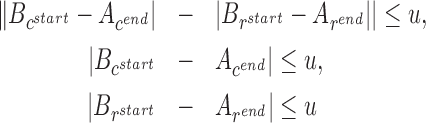The above three cases respectively correspond to inversions, deletions, and duplications/insertions. We have provided an illustrative explanation for these conditions in Supplementary Figure 5. Note that the edges in the DAG are always directed from upstream to downstream based on contig coordinates. If one of the intervals maps to its reverse complement, we exchange the start and end reference coordinates. Finally, we add a ‘source’ and a ‘destination’ vertex with edges to and from every other vertex in the DAG. We set the weight of an edge to be the length of the target interval and 0 weight for edges to the ‘destination’ vertex. The solution of our optimization problem is represented by the longest path in the DAG from the source vertex to the destination vertex. This problem is solvable through a simple greedy algorithm once the vertices are ordered via topological sorting. Figure 2 shows how SViCT builds a DAG for a given set of intervals and how it computes the (one or more) optimal mappings.

Figure 5.

Comparison of SViCT with other popular SV callers in terms of PPV and sensitivity for three simulated cfDNA dataset with 10% ctDNA using various read lengths. Color shading corresponds to sequencing read lengths: 75 (lightest), 100 and 150 bp (darkest). Overall PPV is used for specific SV types for tools that do not classify SVs (GRIDSS and Socrates). Overall PPV is used for Lumpy2 translocations to ensure PPV is not underestimated due to BND entries matching other SV types.

Figure 2.

An example execution of the algorithm for identifying chains of compatible intervals in a multi-mapping contig. (A) The various mappings of the contig to the reference including noise. The central blue bar indicates the contig sequence and the surrounding bars are reference sequences. (B) The topologically sorted, weighted (by length) DAG constructed from the intervals above. Nodes are the intervals and edges are created if two intervals are adjacent (within a given uncertainty) on either the contig or the reference. Superfluous edges from the source and destination to all nodes are removed for clarity. (C) The resulting paths (thick arrows) after finding all co-optimal longest paths (in this case 2) from source to destination through the DAG. The first includes an insertion and deletion on chromosome A and the second includes an insertion and translocation from chromosome B.

Structural variant calling and fusion annotation

The final stage of SViCT interprets optimal contig mappings and predicts structural variants in two steps: (i) Identification of all classes of short SVs as well as deletions and duplications of any length entirely contained within a single contig. (ii) Identification of long structural variants involving two contigs.

Typically a contig has a single ‘breakpoint’ locus (derived from split read and soft-clip mappings), except for those contigs that include a short SV such as an inversion or an insertion, for which there could be additional breakpoints. If indeed the contig has a single breakpoint, step (i) identifies the closest intervals on either side of the breakpoint and checks whether their mapping loci are in close proximity (≤5 kb by default). If they are, and there is a gap between the mapping loci of the two intervals, it declares a deletion. If there is a reversal of the order of the intervals with respect to the mapping loci (see Figure 3), it declares a (likely tandem) duplication. If one of the two sides does not have an associated interval, this indicates a long SV, which is handled in step (ii).

Figure 3.

Different signatures of short SV types detectable by step (i) of variant calling by SViCT. The centre blue bar represents the contig, and the surrounding bars represent various genomic loci. The connecting lines display the various ways the contig can map to these loci.

In case there are two (sufficiently distant) breakpoints, step (i) first checks the possibility of a short inversion by considering the closest intervals to either side of each breakpoint. In case the intervals between the breakpoints have reverse complementary matching loci on the reference genome as per Figure 3, then step (i) calls an inversion. In case there are no intervals between the breakpoints that have an associated mapping locus again as per Figure 3, then step (i) calls an insertion. In case there are intervals between the breakpoints that only have distant mapping loci (>5 kb or in a different chromosome), then step (i) calls a translocation. In the rare case that none of the above apply, then the two breakpoints are treated independently for the possibility of two independent SVs covered by a single contig.

Step (ii) involves identification of longer SVs (other than deletions and duplications), i.e. those that are longer than a contig length—which can only be captured by analyzing pairs of contigs as a joint ‘signature’ of a long SV. These include longer inversions, translocations as well as insertions. For that, step (ii) matches contig pairs for possible signatures for each of these SV types. Figure 4A depicts possible contig pairs produced by translocations and inversions - the signature for insertions are easier to locate as will be described below.

Figure 4.

Illustrative example of the greedy interval pair joining using eight contigs crossing two chromosomes for step (ii) of SV calling by SViCT. (A) The darker colored intervals are ‘outer’ intervals for the lighter colored SV region, and those sharing a color are valid signatures. The lines show the mapping of each interval to the reference chromosomes. (B) These are the corresponding intervals for the Interval Scheduling Problem. Contig 1 cannot be paired to another contig and is not included. (C) Execution of the greedy algorithm where ‘bordered’ intervals are in the output set. Interval 1 (most upstream end point) is selected first. Interval 2 is deleted since it overlaps with interval 1. Interval 3 and 4 are subsequently added and have no overlaps. (D) The resulting SV calls for the compatible pairs of contigs.

In order to achieve this, step (ii) considers all pairs of contigs that could not be handled by step (i) for further analysis as follows. First, it considers pairs of contigs for a long inversion signature (e.g. in Figure 4A, contig 2 could be paired with both contig 3 and contig 5) which consists of a pair of intervals on opposite sides of their corresponding contig breakpoints, each of which mapping near the mapping locus of the opposite contig - in a reverse complementary manner.

Next, step (ii) considers pairs of contigs with proximal mapping loci for a long translocation signature. Such a signature consists of a pair of intervals on opposite sides of their corresponding contig breakpoints, which map proximally to a distant loci (e.g. in Figure 4, contig 7 and contig 8 could be paired for a translocation signature).

Finally, step (ii) considers pairs of contigs that approximately have the same (≤u) breakpoint in terms of reference location, one on each side of the breakpoint, each with a corresponding unmapped suffix or prefix greater than the anchor size (40 bp). Such a contig pair is considered to provide a long insertion signature.

Each contig can give rise to one or more SV signatures. In order to account for the maximum number of such contigs through implied SVs that do not overlap (i.e. are compatible), step (ii) identifies the maximum matching of contig pairs—each indicating an SV signature—whose implied SVs are all compatible (under the assumption that overlapping or nested SVs do not occur; such events have been observed in rare cases (26) but, as per all available SV discovery methods, are excluded by SViCT ). See Figure 4D for examples of compatible SVs implied by pairs of contigs. This can be formulated as a maximum interval matching problem as per below.

Each pair of contigs can be seen as a single, long genomic-interval (not to be confused with the notion of an ‘interval’ within a contig) spanning a chromosomal region as shown in Figure 4B. Finding the maximum number of such non-overlapping genomic-intervals then becomes an instance of the (Genomic) Interval Scheduling Problem (27). The optimal solution can be found using the standard greedy algorithm for finding the maximum independent set of genomic-intervals (28). (Note that it is possible to first commit to all pairs of contigs that indicate an insertion signature since they indicate a genomic-interval of minimum length - implying that the remaining signatures are for inversions and translocations only).

1. Sort all genomic-intervals I by the downstream genomic position

2. Select the first (most upstream) genomic-interval i ∈ I and move it to the result set.

3. Remove all genomic-intervals that overlap with i.

4. Iterate to the next genomic-interval and continue until I = ∅.

An example execution is shown in Figure 4C. The result is the maximum number of compatible intervals representing non-overlapping long SV calls (Figure 4D).

All SVs breakpoints are cross referenced against a GTF annotation file to determine if they are located in a UTR, intronic or exonic region. In cases where the structural variant involves two breakpoints (deletions, inversions, interspersed duplication), each breakpoint has a separate annotation, as well as the region in between the breakpoints. For example, if an entire exon is deleted but both breakpoints fall in the flanking introns, the call will be annotated as exonic and intronic. For translocations, regions on either side of the breakpoint are annotated separately. If breakpoints are located in intronic/exonic regions from two distinct genes, SViCT will additionally annotate the SV as a fusion. The SV breakpoint coordinates, contig information (including support) and annotation are printed in standard VCF format.

RESULTS AND DISCUSSION

We evaluate the performance of SViCT on both simulated and real data. The simulated cfDNA dataset was created by generating reads from a reference with a wide variety of inserted SVs. The real data includes the Horizon and SeraCare reference datasets containing experimentally validated SVs. We used the former to compare with existing SV callers and used the tool with best performance for comparison in real data. Additionally, we analyzed eight CRPC patient samples in order to discover novel structural variants. Tools were assessed on positive predictive value (PPV), sensitivity and execution time.

Simulation of cfDNA datasets

In order to assess the performance of SViCT , we created a simulated cfDNA dataset with inserted deletions, insertions, inversions, duplications (tandem and interspersed) and translocations (balanced, indel, and duplication). The first step in generating this dataset was to create the donor reference with SVs. We begin with the Venter genome and create three references: normal, tumor allele1 and tumor allele2. Normal is exactly the Venter genome, allele1 contains all the SVs and allele2 contains a subset of the SVs in order to simulate heterogeneity. Since we will be simulating a targeted panel, SVs were only inserted into regions where at least one breakpoint falls in an exonic region of some gene in the gene panel. The algorithm to insert the SVs works as follows. Every exon is randomly selected to contain a breakpoint or not. The breakpoint is then randomly assigned a SV type, short/long, both/allele2 and tandem/interspersed (for duplications). If ‘short’ is selected, a length is randomly generate between 10 and 1000. This may lead to a breakpoint occurring in an intronic region. If ‘long’ is selected, a second location is selected within an adjacent exon that is less than 10kb away or, if no such exon exists, a length of 1–10 kb is randomly selected. Any time a long insertion or long interspersed duplication is generated, it has a random chance of being added to a pool of breakpoints to be used to generate translocations. These are then randomly joined to create the three kinds of translocations mentioned above, including both interchromosomal and intrachromosomal events. This resulted in 760 SVs, evenly distributed between different types. Because of the re-classification of long insertions and duplications, the distribution appears to be skewed towards translocations. By our definition of translocations, we believe this should be viewed as a type encompassing large scale cases of the other types, and therefore would be expected to be more numerous than the other individual types.

The second step was to generate reads using the newly created references. This was done using the tool Wessim2 (29) for simulating whole exome sequencing reads, since, to our knowledge, there is no read simulator tailored for the targeted sequencing used for cfDNA. Wessim2 requires three inputs: the reference, probe sequences and an error model. 6218 probes were obtained from Agilent Technologies for a custom design created using Agilent SureDesign (https://earray.chem.agilent.com/suredesign/). This design is approximately equivalent to the Comprehensive Cancer Design, including 105 of the 107 genes (UTRs, exons and introns). The error model was created using GemSIM v1.6 (30) for the MiSeq v3 paired-end sequencing protocol. The parameters used for Wessim2 were -f 200 -d 100 -m 100, representing the fragment size, fragment size standard deviation and minimum fragment length, respectively. Read length was specified with -l, with values 75, 100 and 150. The fragment length parameters allow us to simulate DNA fragmentation. The parameters were selected to produce a distribution of fragment lengths close to that observed in real cfDNA datasets. We selected four dilutions, 10%, 1%, 0.5% and 0.01%, for generating our simulated samples. For the 10%, 1% and 0.5% dilutions, 4 million reads of each read length were created from allele1/allele2 combined. For the 0.01% dilution, 70 million reads were required to be generated in order to achieve 2x ctDNA coverage. This resulted in approximately 1500× overall maximum coverage (26 000× for 0.01%), 150× for the ctDNA fraction at 10% dilution (approximately 15×, 7×, 2× for the other dilutions, respectively) for the 100 bp read samples. The 150 and 75 bp read length samples have higher and lower coverage, respectively, of ∼±500× (and a proportional difference in the dilutions). The reads were mapped using BWA mem (25) with all default parameters.

Performance comparison

No SV detection tools currently exist which are tailored to cfDNA data, and so we used popular, general purpose SV callers for comparison. We compared SViCT to Delly2, Pindel, GRIDSS, Socrates and Lumpy2 in terms of PPV and sensitivity. In this context, PPV is computed as the ratio of the number of true positives (predicted breakpoint is within 10 bp of a real breakpoint) and the total number of true positives and false positives (all other calls). Sensitivity is computed as the ratio of the number of true positives and the total number of true positives and false negatives (number of inserted SVs). Due to the uneven coverage of targeted sequencing, SV breakpoints may not have sufficient coverage to be detectable, and so they are excluded from this calculation. The total number of calls with coverage are 670, 630, 528 and 289 for 10%, 1%, 0.5% and 0.01% dilutions respectively.

We carefully examined the parameters of each tool for potential optimizations for cfDNA data. Specifically, we modified any applicable parameter, re-ran the tool on the 150 bp, 10% sample, and compared the results in terms of F-score (harmonic mean of PPV and sensitivity) with those obtained when using the default parameters. Only Pindel benefited from these optimizations and so all other tools were executed with default parameters for all experiments. For Pindel, we selected -H 10 -m 10 -M 2 -x 5, which correspond to minimum soft-clip length, minimum anchor length, minimum support and maximum SV length, respectively. The first three parameters massively reduced the number of false positives with no loss in true positives. The forth was adjusted for Pindel to be able to detect even the longest SVs in our simulation (SVs up to 32 368 bp) and improved both PPV and sensitivity. Note there is an option for predicting long insertions, however we opt not to use it as it reduced pindels’ precision since it produces 50% more false positives for only 16 additional true positives.

Due to the difficulty of discovering structural variants with such a low signal, the focus here is on sensitivity. Specifically, we did not filter the results of any of the tools, except GRIDSS where many low support calls (LOW_QUAL) could be removed without affecting the sensitivity. Also Pindel does not predict translocations and so this SV type is excluded when calculating metrics for this tool. SViCT , Lumpy and GRIDSS produce output in VCF which may have breakend (BND) entries (see documentation at https://samtools.github.io/hts-specs/VCFv4.2.pdf). These are ambiguous in terms of the type of SV so they are matched to all SV types. Socrates uses its own output format which also does not classify breakpoints. This creates a challenge for assessing PPV, particularly in Lumpy2 and GRIDSS that heavily rely on BND entries. For GRIDSS and Socrates, we can only compute overall PPV, and use this value for each SV type in Figure 5. For Lumpy2, some of the true positive calls explicitly match an SV type, while others are BND entries. For this reason, using all BND calls for computing translocation PPV would underestimate the value, and so we use overall PPV for this SV type in Figure 5. For the other SV types, we only use the explicitly classified calls for computing PPV, and this may overestimate the value. SViCT uses BND entries solely for translocations and so does not have such complications.

We first ran all tools at the highest dilution (10%) as an initial ‘easy’ test and to assess the effect of read length. GRIDSS did the most poorly, particularly in terms of PPV. This could be due to their reliance on OEAs and discordant read pairs, which are less reliable in cfDNA data due to often short and variable fragment lengths. Socrates is the representative tool for using only soft-clipped reads. Its superior performance over GRIDSS demonstrates the importance of using soft-clipped reads to guide cfDNA SV analysis. Lumpy2 fared best out of the compared tools, but SViCT outperformed or matched Lumpy2 in every category. This is accomplished with a competitive execution time shown in Table 1 (Computed using a AMD FX-9590, 16GB RAM, Ubuntu Linux system). Runtime performance is particularly good when compared to Lumpy2 in real data where Lumpy2 takes approximately 50% longer. Most tools were relatively unaffected by changes in read length, with only Lumpy2 and Pindel showing some differences in performance.

Table 1.

Runtime comparison of all the tested SV detection tools on the 10% ctDNA, 100 bp read length, simulated data and HD786 real data

Tool	CPU time
	Simulation	Real
SViCT	3m27s	17m56s
Lumpy2	2m31s	28m45s
GRIDSS	6m14s	48m8s
Socrates	45s	22m5s
Delly	6m57s	7h52m40s
Pindel	9m04s	11h7m42s

It should be noted that the parameters presented in the methods either mainly affect runtime/memory (e.g. k-mer length) or have a typical PPV/sensitivity trade off (e.g. minimum interval length). Since we demonstrate superior F-score by a significant margin, the choice of parameters does not have a major affect on the comparison. In order to provide evidence for this claim, we ran SViCT with various values for anchor length (a), uncertainty (u) and k-mer size (k), and assessed overall PPV and sensitivity. As shown in Supplementary Table 1, there was little difference between the runs. Furthermore, our simulation has a comprehensive set of SV types in a wide range of lengths. This leads us to believe that SViCT would have superior performance on any simulated cfDNA dataset.

Next we ran all tools on datasets with lower ctDNA dilutions. As previously mentioned, this includes 1%, 0.5% and 0.01% ctDNA. We used 100 bp reads for this analysis as it is the median value, and as demonstrated in Figure 5, most tools are robust to changes in read length. The results of this analysis are shown in Figure 6. PPV improved slightly between 1% and 0.5% for SViCT , Lumpy2 and Socrates. Socrates continued to improve at the 0.01% dilution. The remaining tools became less precise as the dilution was reduced. sensitivity drops for most tools as expected, but SViCT retains its margin over other tools across all dilutions. Delly2 showed an increase in sensitivity at the lowest dilution, likely due to the higher overall read coverage. This was also observed for lumpy2 deletions. All other tools were unaffected by the increased number of normal reads. It is particularly impressive that SViCT can retain reasonable performance even at extremely low tumor read counts. This indicates that our tool can handle even the most difficult patient samples.

Figure 6.

Comparison of SViCT with other popular SV callers in terms of PPV and sensitivity for three simulated cfDNA dataset with 100 bp read length using various dilutions. Color shading corresponds to the ctDNA dilution: 0.01% (lightest), 0.5% and 1% (darkest). Overall PPV is used for specific SV types for tools that do not classify SVs (GRIDSS and Socrates). Overall PPV is used for Lumpy2 translocations to ensure PPV is not underestimated due to BND entries matching other SV types.

A total of 49 calls were only included in allele2 in this dataset. SViCT was able to detect 36 of these calls, and the reduction in the number of detected calls fell at a similar rate to calls present in both alleles ( 26, 20, 4 for each dilution respectively). This result shows that, in principle, SViCT handle clone-specific structural variants. Additionally, 14 calls have a breakpoint in an intronic region. These calls did not cause much difficulty, with 10 being successfully identified ( 10, 8, 2 for each dilution respectively). Although our simulation enforced one breakpoint to be exonic, it is not a requirement for detection. SVs can be detected in any region with read coverage, including UTRs and introns. For comparison, Lumpy2 found fewer allele2-only and intronic calls in all dilutions (31, 19, 10, 0 and 9, 7, 5, 0 respectively).

SV detection in real reference data

In order to evaluate SViCT real world performance, we executed it on two real reference datasets. They are designed to assess the sensitivity of custom targeted sequencing assays. To make these datasets, a combination of wild type and variant-containing genomic DNA from standard reference materials is created with known ratios. The reference materials are from Horizon Discovery (HD786 cfDNA at 5% ctDNA and HD753 gDNA normal, obtained from https://www.horizondiscovery.com/reference-standards), and SeraCare (AF5, AF12, AF06 and AF01, corresponding to four allele frequencies, 5%, 1.2%, 0.6% and 0.1%, obtained from https://www.seracare.com/Controls-Reference-Materials). HD786 is created in vitro by mixing ‘donor’ cancer cell lines with ‘recipient’ cell lines of different genotype. The donor-derived cfDNA (dd-cfDNA) is meant to simulate ctDNA. SeraCare samples are created using a series of DNA plasmids harboring known gene variants which are inserted into a well-characterized human genomic background (GM24385) at desired molecular ratios.

All samples were sequenced using custom gene panels designed to target all variants included in Horizon Discovery reference standard, including four experimentally validated structural variants: a deletion, an insertion and two fusions. The deletion (E746_A750delELREA) is also included in the SeraCare reference standard. Illumina NextSeq500 was used to sequence each reference, and repeated to create a replicate. For HD786, all known structural variants have sufficient coverage to be detectable. For the deletion in the SeraCare samples, there is a detectable signal for the 5% and 1.2% dilutions in both replicates, and for 0.6% in one replicate (Run 1). A summary of these datasets is provided in Table 2. These reads were mapped to GRCh38.86 using BWA mem with all default parameters.

Table 2.

Summary of real reference samples, including cfDNA concentration, number of genes in the targeted panel, approximate number of generated paired-end reads and the approximate, per-base, average read coverage. Coverage is not uniform and may vary significantly between genes

Sample	cfDNA	# Genes	# Reads	Average read coverage
Horizon Run 1	20 ng/μl	18	79 million	∼151 000×
Horizon Run 2	20 ng/μl	18	46 million	∼85 000×
SeraCare Run1	10 ng/μl	18	33–56 million	∼87 000×
SeraCare Run2	10 ng/μl	18	44–48 million	∼85 000×

We ran all tools with identical parameters to the simulation run except those to adjust the minimum variant size since the shortest insertion is only 9 bp long. The results for Horizon samples are shown in Table 3. SViCT was able to identify all four variants in HD786. Lumpy2, Socrates and Delly2 were able to identify the fusions, but not the insertion and deletion. Lumpy2 was only able to identify the chr10:43114499 breakpoint, but could not identify the correct fusion partner. Pindel was the only other tool able to identify the insertion and deletion, but produced a very large number of calls. Identical results were obtained between the two replicates. Unfortunately the small number of SVs in this dataset makes it difficult to draw conclusions on performance. However, the ability of SViCT to find all the SVs with a relatively low number of total calls in the Horizon sample certainly suggests it is effective in a real world setting. What is quantifiable is the superior execution time, which demonstrates the utility of the tool for the analysis of large cohorts.

Table 3.

SVs detected by SViCT and compared tools in the Horizon reference data set. Lumpy2 predicted an incorrect fusion partner and Pindel is not designed to predict translocations

Variant Type	Chr	Gene	Variant	SViCT	Lumpy2	GridSS	Socrates	Delly2	Pindel
Deletion	7	EGFR	E746_A750delELREA	Yes	No	No	No	No	Yes
Insertion	7	EGFR	V769_D770insASV	Yes	N/A	No	No	No	Yes
Fusion	4:6	ROS1	SLC34A2/ROS1	Yes	Yes	No	Yes	Yes	N/A
Fusion	10	RET	CCDC6/RET	Yes	Incorrect	No	Yes	Yes	N/A
Total Calls Run 1				3026	9967	1980	1904	4878	94 869
Total Calls Run 2				2105	8881	3463	1900	8972	75 582

Only SViCT was able to predict all four SVs. All tools found/missed the same SVs between the two replicates.

The results for SeraCare samples are shown in Table 4. As noted earlier, in all dilutions where there was a detectable signal, SViCT was able to identify the aforementioned deletion. On these samples, Pindel provided the best performance among the alternative tools we tested, detecting the deletion in both replicates of the 5% dilution and one replicate of the 1.2% dilutions. As with the Horizon data, Pindel produced an enormous amount of calls with an exceedingly long runtime. Delly2 was also able to the detect the deletion, but only in the highest dilution in one replicate. Other tools were unable to identify the deletion. This result provides additional evidence of SViCT ’s ability to detect SVs with ctDNA proportions much lower than 5% in real data. However, in order to assess the accuracy of all tools we tested in a systematic manner, a more comprehensive gold standard dataset could be helpful.

Table 4.

Detection of the deletion (E746_A750delELREA) in EGFR by SViCT and compared tools in the SeraCare reference data set

Replicate	Dilution	SViCT	Lumpy2	GridSS	Socrates	Delly2	Pindel
1–2	5%	Yes	No	No	No	Yes*	Yes
1–2	1.2%	Yes	No	No	No	No	Yes*
1	0.6%	Yes	No	No	No	No	No

Only SViCT was able to detect this deletion at all dilutions with a detectable signal (0.1% does not contain breakpoint spanning reads). An asterisk (*) marks cases where the tool only found the deletion in one of two replicates.

SV detection in prostate cancer patient samples

Our third dataset is targeted sequence data from cfDNA of eight patients with metastatic, castration-resistant prostate cancer (CRPC). A targeted panel was used including 75 prostate cancer related genes, covering exonic regions, UTRs and intronic regions directly flanking exons (with lower coverage). The total cfDNA concentration for each sample was 1,500ng/μl. These samples were sequenced using Illumina NextSeq producing 6–20 million, 2 × 75 bp reads per sample. The reads were mapped to GRCh38.90 using BWA mem with all default parameters. Details of the extraction, preparation, clinical information and specific sequencing depth of these samples are provided in Supplementary File 1. Furthermore, we ran VarDict (31) with default parameters on all samples and matched the results to known SNVs/SNPs from COSMIC (32) in order to provide some insight on ctDNA fractions and potential clones. This information is also included in Supplementary File 1. SViCT was executed on each sample with default parameters. The SV VAF is approximated by comparing the number of reads supporting a breakpoint to the total reads overlapping the breakpoint loci. If an SV has two breakpoints, the sum of the read counts supporting the breakpoints is divided by the sum of the totals. We report if we observe recurrence and/or a call has a corresponding dbSNP (33) or DGV (34) entry.

SViCT predicted 1147 calls across all eight samples. Calls with low support (<3 reads, 682 calls), and those mapping to intergenic regions (147 calls), and repeat regions (314 calls) were filtered out. This yielded four high confidence SV calls shown in Table 5. These calls have a high number of uniquely mapping, breakpoint-spanning reads. This includes a novel tandem duplication in PIGU, two deletions in PTEN and IKBKB, and an insertion in TMPRSS2. PIGU (Phosphatidylinositol Glycan Anchor Biosynthesis Class U) encodes a cell membrane protein that regulates cell division and growth (35). PIGU is overexpressed in bladder (36), breast (37) and prostate (38) cancers and has evidence supporting its oncogenic role in these cancers. The duplication creates a copy of the first exon, without the start codon and six following base pairs, ∼100 bp into the first intron (Figure 7). The duplication excludes precisely three amino acids from the exon, so no frameshift would be produced if the aberrant transcript is translated. Further investigation would be needed to establish how this could be contributing to the cancer phenotype.

Table 5.

High confidence SV predictions for the eight prostate cancer patient samples

Type	Sample	Gene	Region	Chr	Start	End	Read support	VAF	DGV	dbSNP
Duplication	8	PIGU	Exon	20	34676880	34677076	48	11.58–18.57%	–	–
Deletion	5	PTEN	Intron	10	87893068	87893965	47	64.50%	esv2678342*	–
Deletion	6, 8	IKBKB	Intron	8	42290344	42290377	124, 86	37.2%, 33.7%	–	rs143122536
Insertion	All	TMPRSS2	Intron	21	41470789	41470789	32–60	50.7–60.5%	–	rs112132031

The read support is the number of unique reads only; PCR duplicates are removed. (*) The DGV variant is slightly longer than the one discovered here.

Figure 7.

Illustration of the novel tandem duplication discovered in sample eight of the CRPC cohort rearranging the cancer oncogene PIGU. The duplicated region is colored in green, which contains a part of the first intron and the entire first exon, except the start codon (red) and a few base pairs. A sample of the reads supporting the event is shown at the bottom of the figure.

Since the duplication breakpoints lie close to the exon boundaries, computing the VAF from breakpoint reads is unreliable. In order to investigate this further, we examined the coverage of PIGU exons across all samples. Sample 7 has near-identical coverage of PIGU to sample 8 for exons 2–12 (Supplementary Figure 1) and does not have a duplication predicted in exon 1. Consequently, we used sample 7 as a control to more accurately determine the VAF of this duplication. As can be seen in Supplementary Figure 2, the coverage pattern is identical between the two samples, but sample 8 has a clear gain (mean = 440 reads) between the predicted breakpoints. This difference in coverage is significant when compared to the distribution of all differences between the two samples (Student’s t-test, p < 2.2 × 10⁻¹⁶). Using these differences in coverage, we computed an average VAF of 15.08% (±3.495).

PTEN, IKBKB and TMPRSS2 have well established roles in prostate cancer. PTEN is a tumor suppressor that negatively regulates androgen receptor (39). IKBKB is an inflammation response gene that promotes tumor growth and metastasis (40). As mentioned earlier, TMPRSS2 commonly forms fusions with ETS genes in prostate cancer (15). No such fusions were detected in these samples, which is not surprising given that the breakpoints of these fusions typically occur in intronic regions, most of which have zero coverage in this dataset. These three intronic calls are detectable since they occur directly adjacent to exonic regions. The deletion in PTEN is upstream of second exon of the gene (Figure 8) and is slightly shorter than the known germline variant esv2678342. The deletion in IKBKB is downstream of exon four and exactly matches the germline variant rs143122536. The insertion in TMPRSS2, occurring directly downstream of exon eleven (Figure 9), was observed in all samples. Since this region of TMPRSS2 is generally unimportant for its oncogenic role, this variant likely has no effect on the phenotype.

Figure 8.

Illustration of the deletion discovered in sample five of the CRPC cohort in the tumor suppressor PTEN. The deleted region is colored in green, which falls in intron one upstream of the second exon. A sample of the reads supporting the event is shown at the bottom of the figure.

Figure 9.

Illustration of the insertion discovered in all samples of the CRPC cohort in the gene TMPRSS2. The inserted region is colored in green, which falls in intron ten downstream of exon eleven. A sample of the reads supporting the event is shown at the bottom of the figure.

We also ran Lumpy2 on the same eight samples with default parameters. Lumpy2 was able to identify the duplication and deletions, but not the insertion. Furthermore Lumpy2 made over 47 000 predictions across the eight samples, while SViCT predicted 1147, indicating a much higher false positive rate. Indeed on closer inspection, many of Lumpy2’s high confidence calls are false positives caused by misinterpretation of long fragments or over-estimation of support due to PCR duplicates. The former is apparent from a very large number of deletion predictions with no breakpoint spanning reads. The latter case can be seen on investigation of the supporting reads, which all have identical sequence in many instances. PCR duplicates can be remove using tools such as Picard (http://broadinstitute.github.io/picard), but even with such filtering Lumpy2 predicted over 9000 SVs while SViCT predicted 375 without loss of the high confidence calls. There were no high confidence calls in the 9000 SVs that were not also identified by SViCT . This result demonstrates that even excellent tools such as Lumpy2 can be confounded by the unusual properties of cfDNA. In this pilot study, SViCT was able to discover known structural variants and a potentially novel duplication. Analysis of larger cohorts will reveal the true utility of SViCT , but these results certainly suggest the tool can successfully detect structural variants using cfDNA.

Identification of genomic alterations is becoming increasingly important in the treatment paradigm of patients with metastatic prostate cancer. As oncologists perform earlier genomic testing during the disease course, identifying mutations and structural variations that can potentially make tumors susceptible to certain targeted and biologic therapies is of paramount importance. Moreover, identifying the evolution of mutations over time through serial liquid biopsies will give further insight regarding the optimal treatment of each patient with metastatic prostate cancer in the era of precision medicine. We believe that existing approaches designed for typical sequencing data from solid tumor biopsies are insufficient to accurately identify SVs in this context. SViCT improves on these approaches, with superior performance on a wide range of ctDNA dilutions and read lengths, both in simulated and real data. This suggests that SViCT can robustly handle the variability expected in clinical setting and be an effective tool for personalized medicine.

The largest limitation of this approach for clinical application is the sequencing itself. For cases with very low ctDNA signal the allele frequency may be close to the error rate. Furthermore, the reliance on PCR may result in false signals from early PCR errors and biases. One way to resolve these issues is through the use of unique molecular identifiers (UMIs) which are random sequences (barcodes) of fixed length appended to DNA molecules prior to amplification (41). The aim is to be able to cluster reads which were derived from the same molecule through these barcodes. After clustering, PCR duplicates and sequencing errors can be effectively removed, typically by determining a consensus read for each cluster. Tools such as UMI-Tools (42) and Calib (43) can accomplish this task. This increases confidence in predictions made with very low allele frequency. Using such barcoding techniques would improve the utility of SViCT under these circumstances.

CONCLUSION

Here we demonstrated that SViCT can efficiently and effectively handle sequencing data from cfDNA samples. It is resilient to high read depth since all reads are essentially ‘collapsed’ into contigs. Reasonable sensitivity is maintained even at very low dilutions of ctDNA with the ability to detect SV signatures with as little as two reads. The good sensitivity can, in principle, allow for detection of allele-specific or clone-specific SV signatures, provided paired normal data is available for accurate VAF estimation. This is achieved while producing fewer false positives than any other tool, removing the need for additional filtration. Finally, the ability of the algorithm to find a small set of optimal interval sets for each contig makes it robust in terms of noise. For these reasons, SViCT is another step toward a comprehensive suite of tools for analyzing cfDNA. This, and other efforts in cfDNA analysis, will help progress precision medicine and reduce reliance on dangerous and invasive biopsies.

DATA AVAILABILITY

The simulation datasets can be accessed through our github repository (https://github.com/vpc-ccg/svict), and the ground truth is provided in Supplementary File 2. Raw sequencing data have been deposited with links to BioProject accession number PRJNA521544 in the NCBI BioProject database (https://www.ncbi.nlm.nih.gov/bioproject/).

SUPPLEMENTARY DATA

Supplementary Data are available at NAR Online.

FUNDING

Natural Sciences and Engineering Research Council Discovery Grant [to F.H.]; Terry Fox Research Institute New Frontiers Program Project Grant [1062 to F.H., C.C.C., S.C.S.]; Natural Sciences and Engineering Research Council Discovery Frontiers Program on the Cancer Genome Collaboratory [to F.H., S.C.S.]; National Science Foundation grant [CCF-1619081 to S.C.S.]; National Institutes of Health grant [GM108348 to S.C.S.]; Indiana University Grant Challenges Program, Precision Health Initiative [to S.C.S.]. Funding for open access charge: Natural Sciences and Engineering Research Council Discovery Grant.

Conflict of interest statement. None declared.

REFERENCES

- 1. Mandel P., Metais P.. Les acides nucleiques du plasma sanguin chez l’homme. CR Acad. Sci. Paris. 1948; 3–4:241–243. [PubMed] [Google Scholar]
- 2. Thierry A.R., El Messaoudi S. Gahan P.B., Anker P., Stroun M.. Origins, structures, and functions of circulating DNA in oncology. Cancer Metastasis Rev. 2016; 35:347–376. [DOI] [PMC free article] [PubMed] [Google Scholar]
- 3. Stroun M., Anker P., Maurice P., Lyautey J., Lederrey C., Beljanski M.. Neoplastic characteristics of the DNA found in the plasma of cancer patients. Oncology. 1989; 46:318–322. [DOI] [PubMed] [Google Scholar]
- 4. Mouliere F., El Messaoudi S., Gongora C., Guedj A. S., Robert B., Del Rio M., Molina F., Lamy P. J., Lopez-Crapez E., Mathonnet M. et al.. Circulating Cell-Free DNA from colorectal cancer patients may reveal high KRAS or BRAF mutation load. Transl Oncol. 2013; 6:319–328. [DOI] [PMC free article] [PubMed] [Google Scholar]
- 5. El Messaoudi S., Mouliere F., Du Manoir S., Bascoul-Mollevi C., Gillet B., Nouaille M., Fiess C., Crapez E., Bibeau F., Theillet C. et al.. Circulating DNA as a strong multimarker prognostic tool for metastatic colorectal cancer patient management care. Clin. Cancer Res. 2016; 22:3067–3077. [DOI] [PubMed] [Google Scholar]
- 6. Wan J.C.M., Massie C., Garcia-Corbacho J., Mouliere F., Brenton J.D., Caldas C., Pacey S., Baird R., Rosenfeld N.. Liquid biopsies come of age: towards implementation of circulating tumour DNA. Nat. Rev. Cancer. 2017; 17:223–238. [DOI] [PubMed] [Google Scholar]
- 7. Vasioukhin V., Anker P., Maurice P., Lyautey J., Lederrey C., Stroun M.. Point mutations of the N-ras gene in the blood plasma DNA of patients with myelodysplastic syndrome or acute myelogenous leukaemia. Br. J. Haematol. 1994; 86:774–779. [DOI] [PubMed] [Google Scholar]
- 8. Sorenson G.D., Pribish D.M., Valone F.H., Memoli V.A., Bzik D.J., Yao S.L.. Soluble normal and mutated DNA sequences from single-copy genes in human blood. Cancer Epidemiol. Biomarkers Prev. 1994; 3:67–71. [PubMed] [Google Scholar]
- 9. Thierry A.R., Mouliere F., El Messaoudi S., Mollevi C., Lopez-Crapez E., Rolet F., Gillet B., Gongora C., Dechelotte P., Robert B. et al.. Clinical validation of the detection of KRAS and BRAF mutations from circulating tumor DNA. Nat. Med. 2014; 20:430–435. [DOI] [PubMed] [Google Scholar]
- 10. Bennett C.W., Berchem G., Kim Y.J., El-Khoury V.. Cell-free DNA and next-generation sequencing in the service of personalized medicine for lung cancer. Oncotarget. 2016; 7:71013–71035. [DOI] [PMC free article] [PubMed] [Google Scholar]
- 11. Wyatt A.W., Azad A.A., Volik S.V., Annala M., Beja K., McConeghy B., Haegert A., Warner E.W., Mo F., Brahmbhatt S. et al.. Genomic alterations in cell-free DNA and enzalutamide resistance in castration-resistant prostate cancer. JAMA Oncol. 2016; 2:1598–1606. [DOI] [PMC free article] [PubMed] [Google Scholar]
- 12. Thierry A.R., El Messaoudi S., Mollevi C., Raoul J.L., Guimbaud R., Pezet D., Artru P., Assenat E., Borg C., Mathonnet M. et al.. Clinical utility of circulating DNA analysis for rapid detection of actionable mutations to select metastatic colorectal patients for anti-EGFR treatment. Ann. Oncol. 2017; 28:2149–2159. [DOI] [PubMed] [Google Scholar]
- 13. Xu T., Kang X., You X., Dai L., Tian D., Yan W., Yang Y., Xiong H., Liang Z., Zhao G.Q. et al.. Cross-platform comparison of four leading technologies for detecting EGFR mutations in circulating tumor DNA from non-small cell lung carcinoma patient plasma. Theranostics. 2017; 7:1437–1446. [DOI] [PMC free article] [PubMed] [Google Scholar]
- 14. Snyder M.W., Kircher M., Hill A.J., Daza R.M., Shendure J.. Cell-free DNA comprises an in vivo nucleosome footprint that informs its tissues-of-origin. Cell. 2016; 164:57–68. [DOI] [PMC free article] [PubMed] [Google Scholar]
- 15. Tomlins S.A., Laxman B., Dhanasekaran S.M., Helgeson B.E., Cao X., Morris D.S., Menon A., Jing X., Cao Q., Han B. et al.. Distinct classes of chromosomal rearrangements create oncogenic ETS gene fusions in prostate cancer. Nature. 2007; 448:595–599. [DOI] [PubMed] [Google Scholar]
- 16. Hormozdiari F., Alkan C., Eichler E.E., Sahinalp S.C.. Combinatorial algorithms for structural variation detection in high-throughput sequenced genomes. Genome Res. 2009; 19:1270–1278. [DOI] [PMC free article] [PubMed] [Google Scholar]
- 17. Fan X., Abbott T.E., Larson D., Chen K.. BreakDancer - identification of genomic structural variation from Paired-End read mapping. Curr. Protoc .Bioinformatics. 2014; 45:doi:10.1002/0471250953.bi1506s45. [DOI] [PMC free article] [PubMed] [Google Scholar]
- 18. Schroder J., Hsu A., Boyle S.E., Macintyre G., Cmero M., Tothill R.W., Johnstone R.W., Shackleton M., Papenfuss A.T.. Socrates: identification of genomic rearrangements in tumour genomes by re-aligning soft clipped reads. Bioinformatics. 2014; 30:1064–1072. [DOI] [PMC free article] [PubMed] [Google Scholar]
- 19. Layer R.M., Chiang C., Quinlan A.R., Hall I.M.. LUMPY: a probabilistic framework for structural variant discovery. Genome Biol. 2014; 15:R84. [DOI] [PMC free article] [PubMed] [Google Scholar]
- 20. Cameron D.L., Schroder J., Penington J.S., Do H., Molania R., Dobrovic A., Speed T.P., Papenfuss A.T.. GRIDSS: sensitive and specific genomic rearrangement detection using positional de Bruijn graph assembly. Genome Res. 2017; 27:2050–2060. [DOI] [PMC free article] [PubMed] [Google Scholar]
- 21. Ye K., Schulz M.H., Long Q., Apweiler R., Ning Z.. Pindel: a pattern growth approach to detect break points of large deletions and medium sized insertions from paired-end short reads. Bioinformatics. 2009; 25:2865–2871. [DOI] [PMC free article] [PubMed] [Google Scholar]
- 22. Rausch T., Zichner T., Schlattl A., Stutz A.M., Benes V., Korbel J.O.. DELLY: structural variant discovery by integrated paired-end and split-read analysis. Bioinformatics. 2012; 28:i333–i339. [DOI] [PMC free article] [PubMed] [Google Scholar]
- 23. Kavak P., Lin Y.Y., Numanagić I., Asghari H., Güngör T., Alkan C., Hach F.. Discovery and genotyping of novel sequence insertions in many sequenced individuals. Bioinformatics. 2017; 33:i161–i169. [DOI] [PMC free article] [PubMed] [Google Scholar]
- 24. Karp R.M., Rabin M.O.. Efficient randomized pattern-matching algorithms. IBM J. Res. Dev. 1987; 31:249–260. [Google Scholar]
- 25. Li H., Durbin R.. Fast and accurate long-read alignment with Burrows-Wheeler transform. Bioinformatics. 2010; 26:589–595. [DOI] [PMC free article] [PubMed] [Google Scholar]
- 26. Zhang C.Z., Leibowitz M.L., Pellman D.. Chromothripsis and beyond: rapid genome evolution from complex chromosomal rearrangements. Genes Dev. 2013; 27:2513–2530. [DOI] [PMC free article] [PubMed] [Google Scholar]
- 27. Spieksma F.C. On the approximability of an interval scheduling problem. J. Scheduling. 1999; 2:215–227. [Google Scholar]
- 28. Gupta U.I., Lee D.T., Leung J.Y.T.. Efficient algorithms for interval graphs and circular-arc graphs. Networks. 1982; 12:459–467. [Google Scholar]
- 29. Kim S., Jeong K., Bafna V.. Wessim: a whole-exome sequencing simulator based on in silico exome capture. Bioinformatics. 2013; 29:1076–1077. [DOI] [PMC free article] [PubMed] [Google Scholar]
- 30. McElroy K.E., Luciani F., Thomas T.. GemSIM: general, error-model based simulator of next-generation sequencing data. BMC Genomics. 2012; 13:74. [DOI] [PMC free article] [PubMed] [Google Scholar]
- 31. Lai Z., Markovets A., Ahdesmaki M., Chapman B., Hofmann O., McEwen R., Johnson J., Dougherty B., Barrett J.C., Dry J.R.. VarDict: a novel and versatile variant caller for next-generation sequencing in cancer research. Nucleic Acids Res. 2016; 44:e108. [DOI] [PMC free article] [PubMed] [Google Scholar]
- 32. Forbes S.A., Beare D., Bindal N., Bamford S., Ward S., Cole C.G., Jia M., Kok C., Boutselakis H., De T. et al.. COSMIC: High-Resolution cancer genetics using the catalogue of somatic mutations in cancer. Curr. Protoc. Hum. Genet. 2016; 91:1–10. [DOI] [PubMed] [Google Scholar]
- 33. Sherry S.T., Ward M.H., Kholodov M., Baker J., Phan L., Smigielski E.M., Sirotkin K.. dbSNP: the NCBI database of genetic variation. Nucleic Acids Res. 2001; 29:308–311. [DOI] [PMC free article] [PubMed] [Google Scholar]
- 34. MacDonald J.R., Ziman R., Yuen R.K., Feuk L., Scherer S.W.. The database of genomic variants: a curated collection of structural variation in the human genome. Nucleic Acids Res. 2014; 42:D986–D992. [DOI] [PMC free article] [PubMed] [Google Scholar]
- 35. Hong Y., Ohishi K., Kang J.Y., Tanaka S., Inoue N., Nishimura J., Maeda Y., Kinoshita T.. Human PIG-U and yeast Cdc91p are the fifth subunit of GPI transamidase that attaches GPI-anchors to proteins. Mol. Biol. Cell. 2003; 14:1780–1789. [DOI] [PMC free article] [PubMed] [Google Scholar]
- 36. Shen Y.J., Ye D.W., Yao X.D., Trink B., Zhou X.Y., Zhang S.L., Dai B., Zhang H.L., Zhu Y., Guo Z. et al.. Overexpression of CDC91L1 (PIG-U) in bladder urothelial cell carcinoma: correlation with clinical variables and prognostic significance. BJU Int. 2008; 101:113–119. [DOI] [PubMed] [Google Scholar]
- 37. Wu G., Guo Z., Chatterjee A., Huang X., Rubin E., Wu F., Mambo E., Chang X., Osada M., Sook Kim M. et al.. Overexpression of glycosylphosphatidylinositol (GPI) transamidase subunits phosphatidylinositol glycan class T and/or GPI anchor attachment 1 induces tumorigenesis and contributes to invasion in human breast cancer. Cancer Res. 2006; 66:9829–9836. [DOI] [PubMed] [Google Scholar]
- 38. Pflueger D., Terry S., Sboner A., Habegger L., Esgueva R., Lin P.C., Svensson M.A., Kitabayashi N., Moss B.J., MacDonald T.Y. et al.. Discovery of non-ETS gene fusions in human prostate cancer using next-generation RNA sequencing. Genome Res. 2011; 21:56–67. [DOI] [PMC free article] [PubMed] [Google Scholar]
- 39. Nan B., Snabboon T., Unni E., Yuan X.-J., Whang Y.E., Marcelli M.. The PTEN tumor suppressor is a negative modulator of androgen receptor transcriptional activity. J. Mol. Endocrinol. 2003; 31:169–183. [DOI] [PubMed] [Google Scholar]
- 40. Ammirante M., Luo J.L., Grivennikov S., Nedospasov S., Karin M.. B-cell-derived lymphotoxin promotes castration-resistant prostate cancer. Nature. 2010; 464:302–305. [DOI] [PMC free article] [PubMed] [Google Scholar]
- 41. Kivioja T., Vaharautio A., Karlsson K., Bonke M., Enge M., Linnarsson S., Taipale J.. Counting absolute numbers of molecules using unique molecular identifiers. Nat. Methods. 2011; 9:72–74. [DOI] [PubMed] [Google Scholar]
- 42. Smith T., Heger A., Sudbery I.. UMI-tools: modeling sequencing errors in unique molecular identifiers to improve quantification accuracy. Genome Res. 2017; 27:491–499. [DOI] [PMC free article] [PubMed] [Google Scholar]
- 43. Orabi B., Erhan E., McConeghy B., Volik S.V., Le Bihan S., Bell R., Collins C.C., Chauve C., Hach F.. Alignment-free clustering of UMI tagged DNA molecules. Bioinformatics. 2018; doi:10.1093/bioinformatics/bty888. [DOI] [PubMed] [Google Scholar]
Associated Data
This section collects any data citations, data availability statements, or supplementary materials included in this article.
Supplementary Materials
Data Availability Statement