The GEDI Simulator: A Large‐Footprint Waveform Lidar Simulator for Calibration and Validation of Spaceborne Missions

Abstract

NASA's Global Ecosystem Dynamics Investigation (GEDI) is a spaceborne lidar mission which will produce near global (51.6°S to 51.6°N) maps of forest structure and above‐ground biomass density during its 2‐year mission. GEDI uses a waveform simulator for calibration of algorithms and assessing mission accuracy. This paper implements a waveform simulator, using the method proposed in Blair and Hofton (1999; https://doi.org/10.1029/1999GL010484), and builds upon that work by adding instrument noise and by validating simulated waveforms across a range of forest types, airborne laser scanning (ALS) instruments, and survey configurations. The simulator was validated by comparing waveform metrics derived from simulated waveforms against those derived from observed large‐footprint, full‐waveform lidar data from NASA's airborne Land, Vegetation, and Ice Sensor (LVIS). The simulator was found to produce waveform metrics with a mean bias of less than 0.22 m and a root‐mean‐square error of less than 5.7 m, as long as the ALS data had sufficient pulse density. The minimum pulse density required depended upon the instrument. Measurement errors due to instrument noise predicted by the simulator were within 1.5 m of those from observed waveforms and 70–85% of variance in measurement error was explained. Changing the ALS survey configuration had no significant impact on simulated metrics, suggesting that the ALS pulse density is a sufficient metric of simulator accuracy across the range of conditions and instruments tested. These results give confidence in the use of the simulator for the pre‐launch calibration and performance assessment of the GEDI mission.

Key Points

• GEDI's simulator has been validated and found accurate enough for pre‐launch calibration activities

• The uncertainties of the simulator have been quantified and ALS beam density identified as a sufficient measure of accuracy

• Interesting quirks of full‐waveform metrics have been highlighted and investigated

1. Introduction

NASA's Global Ecosystem Dynamics Investigation (GEDI) spaceborne lidar mission, which was successfully launched on the 5th December 2018, will make near global measurements of the Earth's land surface within the orbital bounds of the International Space Station (51.6°S to 51.6°N; Dubayah et al., 2014; Stysley et al., 2016). A number of data products will be derived from the measurements, including ground elevation, canopy height, foliage profiles, and above‐ground biomass density (AGBD). These products will be at higher resolution and with higher accuracy than has been previously possible with spaceborne lidar (Los et al., 2012), enabling a better understanding of terrestrial processes and ecology.

The pre‐launch calibration plan of GEDI requires a tool to simulate GEDI waveforms. This is needed to provide data for pre‐launch calibration of algorithms and to assess the instrument performance as part of an end‐to‐end simulator. In particular, the AGBD algorithm requires GEDI measurements colocated in space and time with ground estimates of AGBD (Drake et al., 2002). GEDI will only be in orbit for 2 years, limiting the use of real data for calibration to ground data collected within a short window of time. A simulator allows data from any site with coincident field AGBD estimates and data suitable for simulating GEDI signals to be used, enabling the exploitation of decades worth of data.

To achieve this the waveform simulator must be able to produce accurate GEDI‐like signals and derived metrics across a broad range of biomes and input data sets. It must also be able to predict the impact of instrument noise on derived accuracy. This paper describes and validates the GEDI simulator to ensure that it can be used in the GEDI calibration and validation plan with confidence.

1.1. Simulating Large‐Footprint Lidar

Large‐footprint, full‐waveform lidars emit short pulses of light to illuminate an area of the ground between 5 and 90 m in diameter. The returned energy is recorded as a function of time to produce a waveform, which is the vertically projected area of scattering surfaces, weighted by their angular reflectances, assuming no multiple scattering (Figure 1). Full‐waveform lidar signals can be simulated from direct measurements of vertical structure from discrete‐return airborne laser scanning (ALS; Blair & Hofton, 1999; Milenković et al., 2017) or terrestrial laser scanning (Hancock et al., 2017), or through a radiative transfer model that makes use of similar structural data (Gastellu‐Etchegorry et al., 2015; Hancock et al., 2012). A method that can be driven by readily available data, without requiring site specific assumptions or rarely collected ancillary data, will ensure that the widest possible range of data can be used in GEDI's pre‐launch calibration. For this reason, terrestrial laser scanning data sets, which cover only small areas, although in much greater detail than possible with ALS, and radiative transfer models, which require ancillary datasets of optical properties and crown structure (Ni‐Meister et al., 2017), were not considered for this study.

Figure 1.

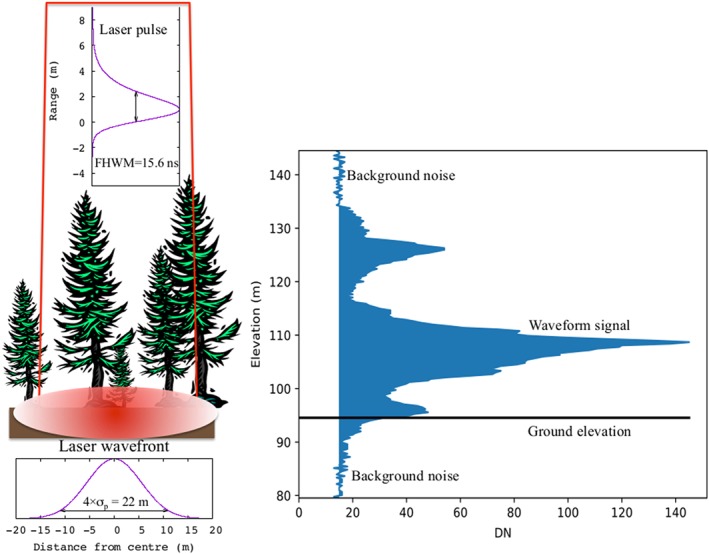
Illustration of Global Ecosystem Dynamics Investigation instrument characteristics and how they contribute to the measured waveform shape.

Discrete‐return, small‐footprint ALS data (referred to as ALS throughout the rest of this paper) has been regularly collected since the 1990s, with many national agencies freely offering data. Discrete‐return lidars employ an almost identical measurement scheme as full‐waveform systems, emitting the same outgoing pulse and receiving the signal with similar detectors. Instead of digitizing the full‐waveform, they use proprietary algorithms to extract a number (typically 1–20) of discrete ranges from the returned energy (Disney et al., 2010) and have footprints typically of between 10 cm and 1 m diameter. This produces an easily interpretable point cloud, where points correspond to the estimated location of scattering surfaces, but in diffuse targets such as vegetation, not all targets are recorded due to the finite length system pulse and dead‐time (Anderson et al., 2016; Disney et al., 2010). Discrete‐return ALS can be converted to a simulation of large‐footprint, full‐waveform lidar data with the method presented in Blair and Hofton (1999) and described in section 2.1. Simulating large‐footprint lidar from discrete‐return ALS assumes that the recorded point cloud is representative of the vertical distribution of scattering surfaces (and so gaps) and ignores multiple scattering of light. While the assumption of the point cloud being representative of the distribution of vertical surfaces has been shown to not be true at the resolution of an individual small‐footprint, ≈30 cm diameter (Hancock et al., 2017), it can be true at the scales of a large‐footprint (>5 m) lidar. Blair and Hofton (1999) compared waveforms simulated from the first‐return only FLI‐MAP ALS (Blair & Hofton, 1999) to observed large‐footprint lidar over the dense tropical forests of La Selva, Costa Rica, and found that their method could accurately recreate the waveform shapes, though with a bias in the ground return energy. Since that study, ALS instruments have improved, with multiple returns per laser shot being recorded and may allow unbiased simulations of large‐footprint waveforms. Note that GEDI's laser beams are generally expected to be less than 6° from nadir so the simulator does not need to be able to precisely simulate large off‐nadir lidar signals.

This paper builds upon Blair and Hofton (1999) in two ways

1. by validating simulations from discrete‐return ALS against observed large‐footprint, full‐waveform lidar data over a wide range of forest and ALS instrument types,

2. by adding instrument noise in order to predict measurement error.

2. Method

Full‐waveform lidar's measurement of vertical structure includes effects from the instrument characteristics (Wagner et al., 2004). These are the laser footprint intensity distribution, system pulse shape, digitizer resolution, digitizer bit rate, and the signal‐to‐noise ratio (SNR). These characteristics are illustrated in Figure 1. The laser footprint intensity distribution is the intensity at each point on the ground, typically a Gaussian defined by the diameter at which the intensity drops to 1/e² of the maximum. The emitted laser pulse is spread over a finite time and a detector has a finite response speed. The convolution of these two effects gives the lidar system pulse and is typically near Gaussian, though can be asymmetric, and is defined by the full‐width half‐maximum or the σ _p width of the Gaussian (FWHM = 2.35×σ _p). The recorded energy is digitized at a finite rate, giving the digitizer resolution of the full‐waveform (typically 1–2 ns). The recorded waveforms are subject to noise from background light, photon shot noise, and electronic noise. Finally, the waveform intensity values plus noise are recorded as digital numbers with the precision quantized to a digital number with a finite digitizer resolution (typically 8–12 bits giving 256–4,096 possible intensity values). The parameters for GEDI and the two Land, Vegetation, and Ice Sensor (LVIS) campaigns used in this paper are given in Table 1. Note that LVIS is configurable and these parameters are only for the LVIS data sets used. These came from the AfriSAR (Lope, Mabounie, and Rabi in 2016), the DESDynI pre‐calibration (Sierra Nevada, Howland, and Hubbard Brook in 2008–2009), and La Selva (1998) campaigns. The La Selva LVIS data were collected in an earlier campaign than DESDynI (Blair & Hofton, 1999), but the characteristics were the same as those during the DESDynI flights and so those data sets have been grouped.

Table 1.

GEDI and LVIS Lidar Characteristics

Instrument	GEDI	LVIS (DESDynI)	LVIS (AfriSAR)
Footprint width (4σ f)	19–25 m	20–24 m	13–22 m
System pulse (FWHM)	15.6 ns	7 ns	11.2 ns
Digitizer resolution	15 cm	30 cm	15 cm
Bit rate	12 bit	8 bit	10 bit
Wavelength	1,064 nm	1,064 nm	1,064 nm
Number of power tracks	4	Scanning	Scanning
Number of coverage tracks	4	NA	NA
Beam sensitivity	92–99.5%	≈98%	≈99.6%
Geolocation accuracy (1σ)	8 m	1 m	1 m
Along track spacing	60 m	Scanning	Scanning
Across track spacing	600 m	Scanning	Scanning
Altitude	400 km	8 km	8 km
Maximum angle of incidence	6°	7° (two flights, 18°)	8°

Note. GEDI = Global Ecosystem Dynamics Investigation; LVIS = Land, Vegetation, and Ice Sensor.

2.1. Discrete‐Return ALS

The simulator follows the method outlined in Blair and Hofton (1999). The laser footprint intensity distribution can be modeled as a Gaussian, weighting the contribution of each ALS point by its distance from the footprint center.

$$I_{w,i}=I_i\frac{1}{{\sigma }_f\sqrt{2\pi }}{e}^{-\frac{{(x_i-x_0)}^2+{(y_i-y_0)}^2}{2{\sigma }_f^2}},$$ (1)

where I _w,i is the weighting of the i ^th point, x _i and y _i are the horizontal coordinates of that point, x ₀ and y ₀ are the horizontal coordinates of the footprint center, and σ _f is the width of the footprint. For non‐Gaussian footprints, the exponential in equation (1) can be replaced by an array of intensity values measured in a laboratory. I _i is a relative weighting of that point to account for any partial hits. There are three options for setting this value. All points could be weighted equally (I _i = 1) ignoring partial hits, as used by Blair and Hofton (1999) and referred to throughout the paper as “count.” Points could be weighted by the number of hits each beam records (I _i = 1/nHits), which assumes that each hit along a laser beam intersects a surface of equal area, as used by Armston et al. (2013) and referred to as “frac.” Finally, it can be assumed that the return laser intensity recorded by ALS systems is proportional to the surface area intersected, as used by Hancock et al. (2017) and referred to as “int.” This last assumption is valid for full‐waveform lidar but is often not the case for discrete‐return systems over diffuse targets (Hancock et al., 2015).

Each point is convolved by the system pulse shape, p(z), along the range axis to produce the ideal waveform, I(z). The convolution can be performed before or after binning. Convolving before prevents aliasing for systems with pulse lengths short compared to the sampling interval, but is more computationally expensive. Convolving after allows much faster operation and that option is tested here.

$$I(z)={\displaystyle \sum _i^N}{I}_{w,i}\otimes p(z-z_i),$$ (2)

where N is the number of ALS points in this footprint and z _i is the elevation of the i ^th point. For a Gaussian system pulse of width σ _p this is given by

$$p(z-z_i)=\frac{1}{{\sigma }_p\sqrt{2\pi }}{e}^{-\frac{{(z-z_i)}^2}{2{\sigma }_p^2}}.$$ (3)

For an asymmetric pulse the shape can be read from a measured array instead of using equation (3). If convolving each point individually, the result of equation (2) is binned to the correct digitizer resolution to produce a noise‐free simulated waveform.

For a given simulated footprint, the ALS pulse density will be variable due to varying scan angles and flight‐line overlap. It could be the case that there are more ALS points from one part of the footprint, giving that part a disproportionate effect on the simulated waveform. This can be corrected by weighting the contribution of each ALS point by the inverse of the pulse density at that point. The pulse density at a point was calculated as the number of last returns vertically projected onto a 1.5‐m grid.

Separate simulated waveforms can be made from ALS points classified as ground and canopy to distinguish the ground and canopy portions of the waveform (examples will be shown in Figure 4). This allows ground‐finding algorithms to be tested in terms of ground elevation accuracy and total extent of the ground energy, required for estimates of canopy cover (Armston et al., 2013; Tang & Dubayah, 2017) and slope (Mahoney et al., 2014).

Figure 4.

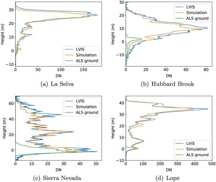
Comparison of four individual simulated and observed LVIS waveforms with the ground portion of the simulated waveform shown. LVIS = Land, Vegetation, and Ice Sensor; ALS = airborne laser scanning; DN = digital number. Examples are shown for La Selva (a), Hubbard Brook (b), Sierra Nevada (c), and Lope (d).

2.2. Noise

Lidar waveforms contain noise from background light and electronic noise. The signal intensity above this noise is controlled by the laser power, surface reflectance, atmospheric attenuation, receiver telescope size, instrument optical efficiency, and the detector efficiency (Wagner et al., 2004). The expected performance of GEDI has been calculated, given the known laser power, optical efficiencies, mean atmospheric transmission at 1,064 nm, expected canopy and ground reflectance, a range of background illumination intensities, and the detector response, as modeled by Davidson and Sun (1988). This provided an expected background noise distribution and an expected return signal strength above that, to give the SNR.

Lidar's SNR can be given in terms of a link margin; that is, the ratio between a threshold set to give a certain probability of background noise being above it (false positive), t _n, and a threshold set to give a certain probability of true signal being below it (false negative), t _s, in decibels (Geng et al., 2015). For white Gaussian noise, all points in a waveform will have a random value drawn from a Gaussian added, producing the noised waveform (as in Figure 1). The probability of a given intensity threshold either including or excluding a feature can be calculated from the cumulative Gaussian distribution. For sections of pure noise, this Gaussian is centered on the mean noise level, and for sections with real signal, the Gaussian is centered on the intensity of the real return. Note that this assumes that photon shot noise (Davidson & Sun, 1988) is constant with varying return intensity. When predicting measurement error, we are interested in low‐intensity parts of the waveform, where the shot noise is at its lowest (Davidson & Sun, 1988). Therefore, it is hoped that this assumption is conservative. This will be tested in section 4.3. A waveform with white Gaussian noise added to a true return, and the resulting noise and signal thresholds, is illustrated in Figure 2.

Figure 2.

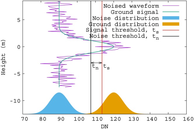
Illustration of link margin for defining the noise level. t _n is set to give a 5% chance of there being a part of the background noise distribution above it within a 30‐m window (false positive). t _s is set to give a 10% chance of the peak of the ground return distribution being beneath it (false negative).

For GEDI, the signal threshold, t _s, was set to a level that gives a 10% probability of a false negative (i.e., 10% of the Gaussian distribution, centered on the signal amplitude, is below that threshold) and the noise threshold, t _n, was set to give a 5% probability of a false positive across a 30‐m window. Note that each waveform bin has a given probability of being a false positive (fraction of Gaussian centered on mean noise level above t _n), so the total probability within a window is the probability of each bin, multiplied by the number of bins; that is, 30 m / digitizer resolution × integral of Gaussian above noise threshold. This gives a probability per waveform bin of 5%/(30/0.15) = 0.025%. The ratio of these two thresholds, in decibels, gives the link margin, linkM.

$$linkM=10\times lo{g}_{10}\left(\frac{t_s}{t_n}\right).$$ (4)

2.2.1. Beam Sensitivity

The link margin can also be expressed in terms of a beam sensitivity, that is, the canopy cover that we would expect to be able to detect the ground through 90% of the time with a 5% chance of a false positive. The amplitude of a ground return, μ _g, with a 0 db link margin can be related to the noise distribution width, σ _n, by calculating the intensity of a real return needed to make t _n = t _s.

$${\mu }_g={\sigma }_n\times 4.76,$$ (5)

where 4.76 is the number of standard deviations between two Gaussian distributions needed for the noise and signal thresholds (t _n and t _s) to be equal for the 5% false positive and 10% false negative rates used for GEDI. The beam sensitivity is then the fraction of energy contained within a Gaussian with this peak amplitude. In percent this is given by

$$b_s=\left(1-\frac{{\mu }_g{\sigma }_{eff}\sqrt{2\pi }}{{\sum }_{-\infty }^{\infty }I(z)-\overline{n}}\right)\times 100,$$ (6)

where $\overline{n}$ is the mean noise level and σ _eff is the ground return's effective width. σ _eff can be calculated from the system pulse width (convolution of transmitted pulse with receiver response), σ _p, the footprint width, σ _g, and the ground slope, θ. This equation can be inverted to calculate ground slope from return width, in a similar way to Mahoney et al. (2014), but without the need for empirical calibration.

$${\sigma }_{eff}=\sqrt{{\sigma }_p^2+{\sigma }_f^2{\tan }^2(\theta )}.$$ (7)

The beam sensitivity can be used to calculate the probability of a lidar waveform being able to detect the ground through a given canopy cover, as shown in Figure 3. Note that each curves passes 10% on the y axis at the canopy cover equal to the beam sensitivity.

Figure 3.

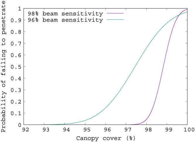
Probability of waveforms to detect the ground against canopy cover for two different beam sensitivities.

2.2.2. Adding Noise to Simulations

Throughout the rest of this paper, instrument noise will be defined in terms of the beam sensitivity. To add noise to waveforms simulated by equation (2), white Gaussian noise with width σ _n is added to all points. σ _n is found by numerically solving equations (4)–(6), and (7) for a given beam sensitivity. A mean offset is then added and the precision truncated to the relevant bitrate. The GEDI power beams are expected to have beam sensitivities of 99.5% by night and 94% by day while the coverage beams are expected to have sensitivities of 96% by night and 92% by day (Table 1). Note that these values assume a loss of 3 db from predictions, to be conservative. LVIS data used in these studies had mean beam sensitivities around 98–99.6% though some individual footprints were found to be as low as 70% in hazy conditions.

2.3. Simulator Conclusion

The above steps were combined with the signal processing and file input/output libraries described in Hancock et al. (2017) to form a simulator in C. The code is available on bitbucket from Hancock (2018) under a Gnu Public License. By changing the values described in Table 1, any downward looking, large‐footprint, full‐waveform lidar instrument can be simulated.

3. Validation Experiments

The simulator was validated against observed large‐footprint, full‐waveform lidar data collected by the LVIS system over a range of forest types and covering a range of ALS systems and sampling densities. The simulator was validated in terms of how well it can recreate waveform metrics derived from real large‐footprint, full‐waveform lidar (section 3.1), how consistent simulated waveform metrics are across a range of ALS survey characteristics for a single site (section 3.2), and how well it can recreate the ground‐finding error statistics of real large‐footprint, full‐waveform lidar (section 3.3).

The data sets used to compare ALS simulations to LVIS (sections 3.1 and 3.3) are listed in Table 2 and the properties of the forests are given in Table 3. La Selva is in Costa Rica, Sierra Nevada, Hubbard Brook, and Howland are in the United States and Lope, Mabounie and Rabi are in Gabon. LVIS has a similar footprint size to GEDI, a shorter pulse length, and a higher beam sensitivity. The higher beam sensitivity means there is less chance of small waveform features being lost in background noise, while the shorter pulse length allows finer resolution of canopy returns, making the waveform more complex. Thus, validating against LVIS is a more stringent test than against GEDI and if the simulator is capable of simulating LVIS accurately, it can simulate GEDI. The ALS data sets covered a range of wavelengths, with the Optech and Leica systems at 1,064 nm while the RIEGL system was 1,550 nm. The Pearson‐correlation maximization method described in Blair and Hofton (1999), with an added simplex optimization for computational speed (Press et al., 1994), showed that the horizontal geolocation of the ALS to LVIS data sets were within 1 m of each other. Remaining vertical datum differences and small horizontal offsets between the ALS and LVIS data sets were corrected by an affine transformation of the ALS data per site.

Table 2.

ALS and LVIS Data Used in Simulator Validation

				ALS pulse	ALS point
Site	LVIS date	ALS date	ALS system	density (m−2)	density (m−2)
La Selva	March 2005	March 2006	Leica ALS50	0.88	1.15
Sierra Nevada	September 2008	September 2008	Optech Gemini	10.6	14.7
Hubbard Brook	August 2009	September 2009	Optech ALTM 3100	2.76	4.02
Howland	August 2009	September 2009	Optech ALTM 3100	3.88	4.82
Lope	February 2016	July 2015	RIEGL VQ480U	7.8	11.1
Mabounie	February 2016	July 2015	RIEGL VQ480U	4.4	4.4
Rabi	February 2016	July 2015	RIEGL VQ480U	4.2	6.0

Note. ALS = airborne laser scanning; LVIS = Land, Vegetation, and Ice Sensor.

Table 3.

Mean Properties of Each Site Within Land, Vegetation, and Ice Sensor Footprints and Number of Land, Vegetation, and Ice Sensor (LVIS) Footprints Used in the Comparison

Site	Biome	Height (m)	Cover (%)	Slope (°)	N samples
La Selva	Evergreen broadleaf	30	81	13.1	178,577
Sierra Nevada	Evergreen needleaf	39	43	13.7	376,677
Hubbard Brook	Deciduous broadleaf	24	90	13.7	186,172
Howland	Deciduous broadleaf	17	76	2.8	265,147
Lope	Evergreen broadleaf	31	75	12.1	573,402
Mabounie	Evergreen broadleaf	36	95	12.6	1,279,272
Rabi	Evergreen broadleaf	34	92	8.4	71,732

3.1. Simulated Waveform Accuracy

Simulations of LVIS‐like waveforms, using the appropriate values for footprint width, pulse shape, beam sensitivity, and digitizer resolution in Table 1, were run for every LVIS footprint location that was covered by ALS data at each site with each of the three ALS point weighting methods (count, frac, and int) and with and without normalizing for ALS pulse density to give a total of six possible simulation methods. The accuracy of the simulated waveforms was quantified by calculating the Pearson‐correlation coefficient between observed and simulated LVIS waveforms (Blair & Hofton, 1999) and by the difference between relative height (RH) metrics (Drake et al., 2002) derived from observed and simulated LVIS waveforms. To ensure that any disagreements were solely due to differences in the simulated waveform shapes, RH metrics were calculated relative to the same ground elevation for both data sets. This was estimated from the original ALS data, using LAStools (Isenburg, 2011).

Past studies have shown that the lower the ALS densities, the greater the chance of the ALS point cloud not penetrating to the ground (Leitold et al., 2015). That would lead to the simulations being inaccurate. This was tested by relating metric differences to ALS pulse density. Similarly, lower beam sensitivity LVIS waveforms may miss weak ground or canopy returns, making them an unreliable truth. To investigate these effects, we related metric differences to LVIS beam sensitivity. Also, the greater the lidar beam zenith angle, the longer the path length through the canopy, which may adjust the vertical distribution of returns. To test for this, differences in waveform metrics were related to LVIS scan angle and the mean scan angle of ALS within an LVIS footprint.

The difference between metrics were compared to surface properties (canopy cover and ground slope) to ensure that the simulator can be used across a range of conditions. Each site was examined separately to identify any differences that might result from the range of forest structures or the different ALS instruments used.

3.2. Simulator Consistency

The validation of simulated LVIS against observed LVIS above used only a single ALS data set per site, collected from a single altitude with uniform scan parameters and laser wavelengths. While the pulse density varied with scan angle and varying overlap between flight‐lines, previous studies have shown that the probability of detecting targets (and so correctly characterizing the foliage profile) depends upon the beam sensitivity of the lidar signal which in turn is controlled by altitude and laser pulse rate (Morsdorf et al., 2008), as well as other factors out of the control of the surveyor. For a given scan rate, the greater the altitude, the lower the pulse density and the larger the footprint will be. A larger footprint has a lower laser intensity for any given point within, potentially meaning that small objects do not return enough signal to trigger a recorded point (such as sparse canopies or the ground under dense canopies). A higher laser pulse rate will give a greater pulse density but less laser energy per pulse, lowering the SNR and potentially preventing the detection of small objects. Laser wavelength may also affect simulation accuracy. Green vegetation has a higher reflectance at 1,064 nm than 1,550 nm, so different amounts of energy will be returned by ground and canopy returns to different wavelength instruments. The waveform shape could potentially be changed if the energy return differences crossed the instrument triggering threshold.

To assess whether varying altitude and laser pulse rate affect the simulated waveform accuracy, LVIS waveforms were simulated using ALS data collected over the Injune Landscape Collaborative Project in Queensland, Australia, on the 20th of August 2015. Data were collected with a RIEGL LMS‐Q560i (1,550 nm laser pulsing at 240 kHz) and RIEGL Q680 (1,064 nm laser pulsing at 400 kHz) at a range of flying altitudes (350–700 m). The canopy was sparse, with a mean cover of 22% and interquartile range of 18% to 41%, calculated from ALS data. At this low cover, canopy returns from lower SNR ALS pulses may be beneath the instrument triggering threshold, potentially causing an underestimate of RH metrics.

Five plots were covered by three or four flight‐lines by each ALS instrument at two or three different flying altitudes. Simulations of LVIS‐like waveforms were made for each flight‐line independently and for all combined to further increase the range of pulse densities. For each ALS instrument, the lowest altitude flight with all flight‐lines combined was used as a benchmark, thus there were two benchmarks. RH from simulations with all combinations of data were compared to the two benchmarks. The RH metric differences were related to pulse density, laser pulse rate, mean scan angle, and altitude to see how consistent the simulated RH metrics were with these survey parameters.

3.3. Simulated Noise Accuracy

The white Gaussian noise used here is an approximation of the true detector noise distribution (Davidson & Sun, 1988). The impact of this approximation on the simulator's ability to predict measurement error was tested. LVIS waveforms were simulated and noise added to give the same beam sensitivities as observed LVIS. Observed LVIS waveforms with low beam sensitivities due to atmospheric attenuation have not been removed to ensure that the simulator is capable of predicting the full range of measurement errors that full‐waveform lidar can suffer. In the GEDI products, these low sensitivity beams would be rejected to avoid errors.

When processing waveform lidar data, algorithms are run to extract and geolocate the ground return. If footprint sensitivities are insufficient and the false alarm rate set too high, then ground elevation errors will occur. To investigate such errors between simulated and observed waveforms, the locations of the lowest modes in observed and simulated LVIS waveforms were extracted using three ground‐finding algorithms. Those were Gaussian fitting, “Gauss” (Hofton et al., 2000), the lowest inflection point, “infl” (zero‐crossing point of the second derivative), and the lowest maximum, “max” (zero‐crossing point of the first derivative). Observed and simulated LVIS waveforms were passed through the same signal processing software to remove noise before applying the ground‐finding method. The signal was smoothed by a Gaussian with a width equal to three quarters of the system pulse and a background noise threshold was set as the mean noise plus 3.5 standard deviations (Hofton et al., 2000). The first and last signal returns were identified as the first and last points with at least three consecutive waveform bins above the noise threshold, tracking back from each until the signal dropped to the mean noise level to avoid truncating real signal (Hancock et al., 2011). Note that this is not the final GEDI ground‐finding algorithm or that used for the LVIS level 2 products.

Ground elevation error was calculated as the difference between the elevation estimated from the noised waveforms (from both simulated and observed LVIS) and the ground elevation estimated from ALS (Isenburg, 2011). The ALS ground elevation estimates were only validated for La Selva, where they were found to have a (root‐mean‐square error) RMSE of 1.66 m against ground‐control survey points (Kellner et al., 2009). Ground elevations at other sites were not validated but past studies suggest that, at the pulse densities of these data sets, ALS can identify the ground elevation to within 1 m through dense forest canopies (Leitold et al., 2015). Ground elevation errors were calculated as a function of the controlling variables, which are beam sensitivity, canopy cover, and slope, from both observed and simulated LVIS waveforms. The errors were binned in to 2% canopy cover, 5° slope, and 2% beam sensitivity intervals and the mean bias and RMSE for each combination calculated. The errors from simulated waveforms were compared to the errors from observed LVIS waveforms in terms of the mean bias, RMSE, and the percentage of variance in error explained.

4. Results and Discussion

4.1. Waveform Accuracy Results

Some examples of simulated and observed LVIS waveforms are shown in Figure 4, showing that they match well visually and illustrating the simulator's ability to isolate the ground portion of the waveform. Of all the factors discussed in section 3.1, ALS pulse density was found to be the main cause of discrepancies between simulated and observed waveforms. Figure 5 illustrates this relationship for the RH50 metrics at four sites (all other RH metrics and the Pearson‐correlation showed a similar trend, other than RH5 and RH98 at some sites, which will be discussed later). At low ALS pulse densities, differences between RH metrics from simulated and observed waveforms were largest. Poor characterization of vegetation is a well known shortcoming of low density ALS (Leitold et al., 2015). For the data available to this study, above a certain density there was no longer a dependence of RH metric accuracy on ALS pulse density. Thus, ALS pulse density seems a sufficient measure to ensure simulator accuracy. An error threshold of 1.5 m absolute median bias and 3 m interquartile range was used to determine minimum usable ALS densities of 1.5 pulses per square meter for the Optech systems over Hubbard Brook and Howland, 3 pulses per square meter for RIEGL systems over Lope, Rabi, and Mabounie and the Optech system over Sierra Nevada, and 0.75 pulses per square meter for the Leica system over La Selva. Repeating Figure 5 with RH98 at Sierra Nevada revealed that RH98 required a higher pulse density threshold than RH50 to ensure no bias (3 pulses per square meter instead of 1.5 pulses per square meter needed by RH50). This is likely caused by low density ALS data missing the tops of conifer trees, Sierra Nevada, being the only coniferous forests tested (Zimble et al., 2003).

Figure 5.

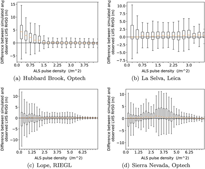
Boxplots showing the difference between RH50 from simulated and observed LVIS waveforms against ALS pulse density for Hubbard Brook (a), La Selva (b), Lope (c) and Sierra Nevada (d). The boxes show the interquartile range (25th and 75th percentile), the bar the median and the whiskers are 1.5 times the interquartile range long. Outliers have been excluded from this plot and will be investigated in detail later, along with the higher root‐mean‐square error at Sierra Nevada around 3.5 pulses per square meter.

Repeating Figure 5 with RH5 and RH2 revealed a 1‐m bias at Sierra Nevada and Howland for all ALS pulse densities. This was not apparent at any other site or for any higher RH metrics. Examining waveforms revealed that this was due to observed LVIS having a longer trailing tail than simulated waveforms. This only occurred in footprints with moderate canopy cover (≈60%), which were most common at Howland and Sierra Nevada and at Sierra Nevada were most common for pulse densities between 2 and 4 pulse per square meter, causing the bias apparent in Figure 5d. The other sites had more bimodal canopy cover distributions with few waveforms over moderate canopy covers. At high canopy covers, no tail was noticeable above background noise and observed and simulated LVIS waveforms matched, possibly because there was insufficient energy at the ground to cause a noticeable tail. Observed and simulated waveforms over bare ground were compared at all sites to make sure that the system pulses being used were appropriate. In all cases, bare ground waveforms matched. The longer tails in observed LVIS could possibly be due to either multiple scattering (when there is sufficient energy reaching the ground with sufficient density foliage to cause scattering) or some electronic detector effect, but further investigation is required to determine the exact cause. In either case, simulated RH5 and below may be biased in moderate canopy covers and cannot be relied upon.

Repeating Figure 5 with ALS data sets decimated by removing a random fraction of all ALS pulses showed that the ALS pulse density thresholds scaled with the level of decimation; a data set with 50% decimation had a threshold 50% of that reported above. This suggests that these thresholds were specific to the survey configurations used here. These thresholds are tentatively proposed as minimum usable ALS densities, but some survey configurations may require different thresholds. Without additional ALS data sets overlapping with LVIS or GEDI data, this cannot be investigated further. Any calibration using simulated data should check whether any outliers in the analysis have low ALS pulse density to check the appropriateness of the above thresholds for that ALS data set.

At some sites, partial cloud cover caused a large range in LVIS's beam sensitivity. For low LVIS sensitivity, areas of low waveform intensity were lost in noise, leading to inaccurate RH metrics. To avoid these errors in observed RH metrics impacting the simulator assessment, a minimum LVIS beam sensitivity of 92% for DESDynI LVIS and 98% for AfriSAR LVIS was set for all further analysis. Above these sensitivities there was no trend in the difference between simulated and observed RH metrics with LVIS beam sensitivity.

LVIS was tested up to a beam zenith angle of 8° at all sites and up to 18° at Sierra Nevada, well above the expected 6° limit of GEDI. The difference between observed and simulated RH metrics showed no consistent bias with LVIS or ALS beam angle, though mean correlation started to decrease above 8°. All further analysis was limited to LVIS footprints with zenith angles less than 8°. The ALS mean scan angle within a footprint reached 30° with no impact on simulator accuracy apparent.

The remaining outliers and waveforms with higher RMSEs at medium pulse density in Figure 5d were examined and some representative examples are shown in Figure 6. Some simulations with large differences between simulated and observed RH50 were for waveforms with a canopy cover around 50%, so that RH50 height was in a section of relatively low intensity (Figure 6a). For RH metrics in areas of relatively low waveform intensity, a very small change in the relative ground to canopy energies would cause a large shift in those RH metrics. The shift distance is directly proportional to the integral of the waveform around that point. For waveforms with large RH50 differences, the other RH metrics tested (RH98, RH75, RH25, RH5, and RH2) all had small differences, as the waveform intensities and integrals were greater than at RH50. Figure 7 shows this ripple of increased uncertainty of RH metrics at canopy covers equal to one minus that RH metric and Figure 8 shows why the shift in RH metric is greatest at areas of relatively low waveform intensity.

Figure 6.

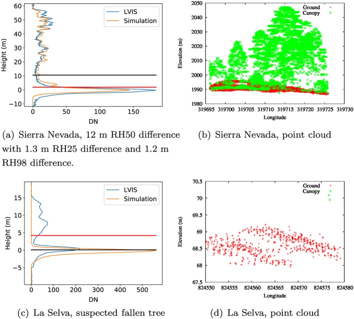
Examples of simulated and observed LVIS waveforms with large RH50 differences. Examples are shown for Sierra Nevada (waveforms (a) and point cloud (b)) and La Selva (waveforms (c) and point cloud (d)). LVIS = Land, Vegetation, and Ice Sensor; DN = digital number.

Figure 7.

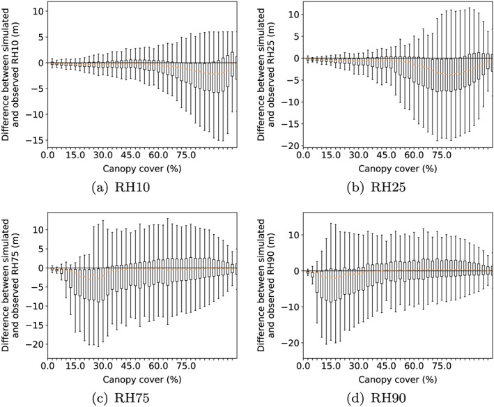
Difference between simulated and observed Land, Vegetation, and Ice Sensor RH metrics against canopy cover over Mabounie, showing a ripple of uncertainty at a canopy cover equal to one minus that RH metric. RH = relative height. Examples are shown for RH10 (a), RH25 (b), RH75 (c), and RH90 (d).

Figure 8.

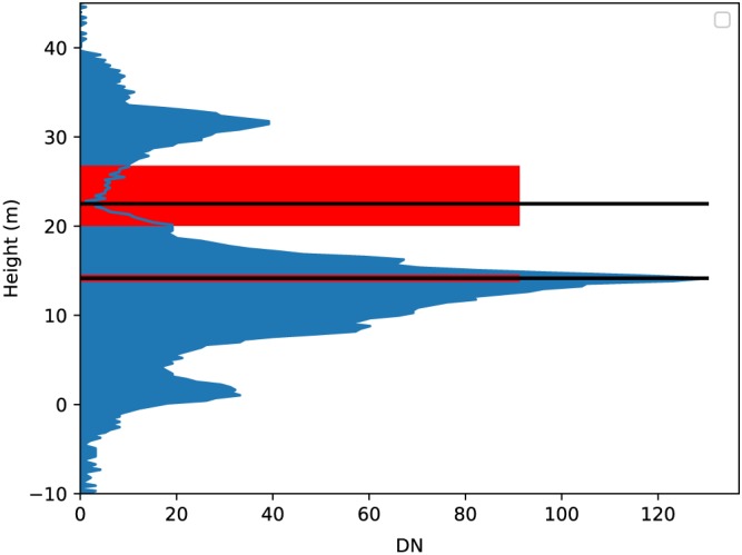
Illustration of distance a 2% change in energy can cause for relative height metrics at points of high and low waveform intensity. Black lines mark RH50 and RH80. Red boxes indicate a shift that would result with a ±2% energy change.

This is a general property of RH metrics and any model using RH metrics will need to take this uncertainty in areas of relatively low intensity into account, as a small change in canopy cover (whether due to leaf wilting, branch dropping or green‐up, etc.) will cause the RH metric around 1‐canopy cover to shift by a large amount without an appreciable change in AGBD (e.g., RH75 for 25% canopy cover and RH25 for 75% canopy cover). A model that uses two or more RH metrics may avoid this issue. Others were clearly due to fallen trees (Figure 6c), but these were too rare to affect the final statistics.

In order to compare the simulator accuracy at all sites and for all RH metrics, histograms of the difference between simulated and observed LVIS RH metrics are shown in Figure 9. For all simulation methods, the mean RH metric difference is submeter with RMSEs around 4.7–5.7 m and correlations around 0.91 (Table 4). All methods had similar RMSEs and correlations, but the lowest bias was achieved with the count method and normalizing for ALS sampling density. This method will be used for the rest of this paper and for GEDI's calibration. Large differences (>5 m) were rare and always explained by one of the cases illustrated in Figure 6.

Figure 9.

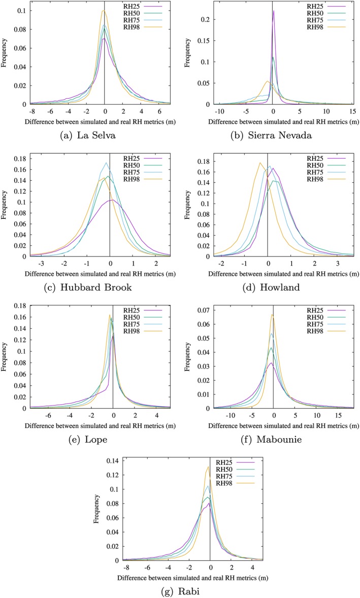
Histograms of difference between observed and simulated Land, Vegetation, and Ice Sensor RH metrics for the count method with airborne laser scanning pulse density normalization. Examples are shown for La Selva (a), Sierra Nevada (b), Hubbard Brook (c), Howland (d), Lope (e), Mabounie (f), and Rabi (g) RH = relative height.

Table 4.

Difference Between RH Metrics From Simulated and Observed Land, Vegetation, and Ice Sensor Waveforms Across All Sites for The Six Possible Simulation Methods

Point	Normalize	Bias			RMSE
weight	ALS density	RH25 (m)	RH50 (m)	RH98 (m)	RH25 (m)	RH50 (m)	RH98 (m)	Correlation
count	Yes	0.06	0.18	0.22	5.61	5.26	4.78	0.909
int	Yes	0.52	0.21	0.21	5.65	5.30	4.75	0.906
frac	Yes	0.54	0.26	0.23	5.60	5.29	4.73	0.909
count	No	0.25	0.54	0.43	5.66	5.30	4.81	0.910
int	No	0.74	0.60	0.44	5.66	5.27	4.78	0.906
frac	No	0.78	0.65	0.45	5.63	5.24	4.76	0.908

Note. RH = relative height; ALS = airborne laser scanning; RMSE = root‐mean‐square error.

That metrics from waveforms simulated from data collected by the 1,550 nm RIEGL VQ480U showed no bias compared to those from the observed 1,064 nm LVIS data, despite the RIEGL having a much lower canopy (green vegetation) reflectance, shows that the SNR of the ALS was sufficient to ensure that the lower reflectance did not place the return intensity beneath the triggering threshold so that the returns were still representative of the foliage profile. The wavelength of discrete‐return ALS does not seem to affect simulation results.

4.2. Simulator Consistency Results

The difference in RH metrics from simulations with ALS at different altitudes, laser pulse rates, and pulse densities were most strongly correlated to pulse density. Figure 10 shows a boxplot of the differences between simulated RH50 from all data sets and the lowest altitude, highest laser pulse rate data set (RIEGL Q680). Results for the lower pulse rate benchmark (RIEGL Q560i) were identical and all other RH metrics showed the same relationship. This shows that there can be large differences at less than 3 pulses per square meter, the same threshold selected for the RIEGL VQ480i in section 4.1. After removing all simulated waveforms with less than 3 pulses per square meter, no trend in RH metric difference was found with pulse density, scan angle, altitude, or laser pulse rate. That there was not an underestimate of RH metrics for the high altitude, high laser pulse rate scans show that even in this sparse canopy, the ALS had sufficient SNR to detect weak canopy returns. Mean RH metric differences were less than 10 cm and RMSEs less than 50 cm. Outliers (greater than 5‐m RH difference) were examined and were explained by either rare data registration issues or else were for RH metrics in areas of relatively low intensity, where a small change in waveform shape can cause a large shift in RH metric position, as in Figure 8. It is concluded that the simulated RH metrics are robust to ALS survey characteristics as long as there is sufficient pulse density, and that the pulse density is an adequate metric of simulator accuracy.

Figure 10.

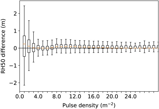
Boxplots of difference between RH50 derived from simulated Land, Vegetation, and Ice Sensor waveforms from airborne laser scanning data sets with different survey configurations over the same site, using the highest laser pulse rate (RIEGL Q680), lowest altitude data set as the baseline.

4.3. Noise Accuracy Results

The noise accuracy analysis included all LVIS beam sensitivities, though low ALS pulse densities and LVIS zenith angles >8° were still excluded. Figure 11 shows a noised waveform with both observed and simulated waveforms showing similar ground‐finding errors. Note that errors this large, in observed or simulated LVIS, are rare cases, as shown by Figure 12. In this case, knowledge of the ground elevation provided by the independent ALS estimate indicates that there was no discernible energy above noise at the expected height (0 m). In both cases a canopy return has been incorrectly selected as the ground, leading to a 20 m inaccuracy for both. This waveform had a beam sensitivity of 66.1%, while the canopy had a cover of 99.7%, so this is not an unexpected results (as shown in Figure 3). In the GEDI products, waveforms that are likely to be unable to see the ground will be flagged as potentially inaccurate and left out of the final gridded products to avoid errors.

Figure 11.

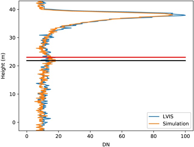
Comparison of ground elevation estimates from observed and simulated LVIS waveforms over Lope. The red line shows the estimate of ground elevation from observed LVIS and the black the estimate from simulated LVIS. This waveform had a canopy cover of 99.7% and a beam sensitivity of 96.1%. LVIS = Land, Vegetation, and Ice Sensor.

Figure 12.

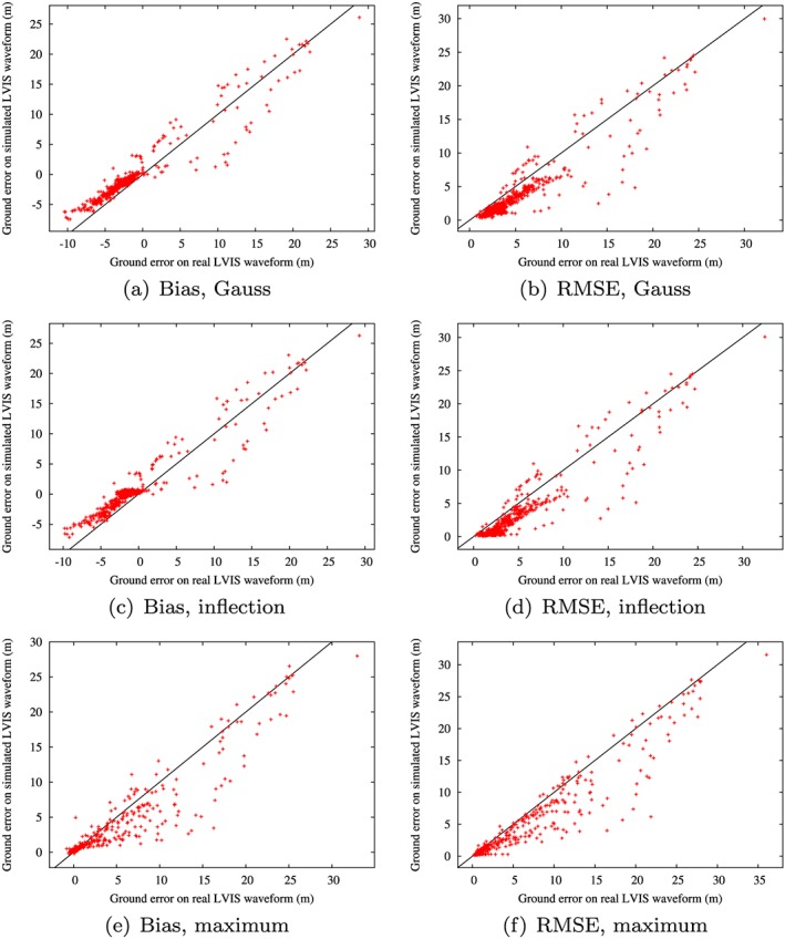
Scatterplots of ground‐finding error on observed and simulated noisy LVIS data, binned by canopy cover, slope, and beam sensitivity across all sites for three ground‐finding algorithms; Gauss (bias (a), RMSE (b)), inflection (bias (c), RMSE (d)), and maximum (bias (e), RMSE (f)). LVIS = Land, Vegetation, and Ice Sensor; RMSE = root‐mean‐square error.

Figure 12 shows scatterplots of the mean bias and RMSE from simulated noised waveforms against those from observed LVIS. Each point represents the mean error for all waveforms within a bin with a given canopy cover (2% intervals), slope (5° intervals), and beam sensitivity (2% intervals). Table 5 shows that the simulator predicted the ground‐finding errors within 2 m of reality and explained over 80% of the variance for the Gaussian and inflection ground‐finding methods, reduced to 67% for the maximum method. In all cases over 70% of the variance in RMSE is explained. The area of the greatest interest is waveforms with beam sensitivities just below the canopy cover, where there is a high chance of ground returns not being distinguishable in the waveforms. The analysis was repeated with just these waveforms and measurement errors from observed and simulated waveforms agreed. Note that the large errors in Figure 12 are for waveforms with beam sensitivities below the canopy cover.

Table 5.

Difference Between Ground‐Finding Error Estimates From Observed and Simulated Land, Vegetation, and Ice Sensor Waveforms in Terms of Mean Bias, RMSE, and as a Percentage of Variance Explained by the Simulations

Method	Bias diff (m)	RMSE diff (m)	Bias var (%)	RMSE var (%)
Gauss	1.37	−1.22	85	72
Inflection	1.59	−1.37	81	71
Maximum	−1.68	−1.96	67	78

Note. RMSE = root‐mean‐square error.

The simulator slightly overestimated the bias in ground elevation and underestimated the RMSE. Separating the scatterplots by canopy cover and slope and examining the raw waveforms revealed that this was because the ground‐finding algorithm triggered on the subterranean tail on observed LVIS (discussed in section 4.1), causing a negative ground elevation error, more often than on simulated LVIS. This was infrequent but occurred often enough to slightly reduce the mean bias from observed LVIS and increase the RMSE. Care should be taken if using the simulated waveforms to assess ground‐finding algorithms and results should be tested against observed large‐footprint lidar data where they overlap.

5. Conclusions

A simulator for generating GEDI measurements, including noise, from any ALS data has been presented. Comparison with observed large‐footprint, full‐waveform data shows the simulator to be accurate for the three most common ALS instrument manufacturers across a wide range of forest types. RH metrics from simulated LVIS waveforms showed less than 0.22 m bias and 5.7 m RMSE compared to observed LVIS waveforms, as long as the ALS data were of sufficient pulse density. Measurement errors due to instrument noise were predicted by the simulator within 1.5 m of those retrieved from observed LVIS waveforms. The uncertainty in simulated metrics is larger for RH metrics in areas of relatively low waveform intensity, but this is a property of RH metrics rather than a limitation of the simulator. The uncertainty has been quantified and will be used as a measure of the simulator accuracy.

Simulations were performed over a single site with a range of ALS survey characteristics, varying flying altitude, laser pulse rate, and flight‐line overlap. This had no significant impact on simulated metrics as long as the ALS pulse density was above the thresholds identified. This suggests that ALS pulse density can be used to quantify simulator accuracy and that simulations with ALS densities above the given thresholds will be accurate.

The simulator code is freely available through bitbucket under a Gnu Public License (Hancock, 2018). It can read any ASPRS las format data and outputs simulated waveforms as ASCII or HDF5 files.

Supporting information

Supporting Information S1

Hancock, S. , Armston, J. , Hofton, M. , Sun, X. , Tang, H. , Duncanson, L. , et al. (2019). The GEDI simulator: A large‐footprint waveform lidar simulator for calibration and validation of spaceborne missions. Earth and Space Science, 6, 294–310. 10.1029/2018EA000506

References

- Anderson, K. , Hancock, S. , Disney, M. , & Gaston, K. J. (2016). Is waveform worth it? A comparison of lidar approaches for vegetation and landscape characterization. Remote Sensing in Ecology and Conservation, 2(1), 5–15. [Google Scholar]
- Armston, J. , Disney, M. , Lewis, P. , Scarth, P. , Phinn, S. , Lucas, R. , Bunting, P. , & Goodwin, N. (2013). Direct retrieval of canopy gap probability using airborne waveform lidar. Remote Sensing of Environment, 134, 24–38. [Google Scholar]
- Blair, J. B. , & Hofton, M. A. (1999). Modeling laser altimeter return waveforms over complex vegetation using high‐resolution elevation data. Geophysical Research Letters, 26(16), 2509–2512. [Google Scholar]
- Davidson, F. M. , & Sun, X. (1988). Gaussian approximation versus nearly exact performance analysis of optical communication systems with PPM signaling and APD receivers. Communications, IEEE Transactions On, 36(11), 1185–1192. [Google Scholar]
- Disney, M. I. , Kalogirou, V. , Lewis, P. , Prieto‐Blanco, A. , Hancock, S. , & Pfeifer, M. (2010). Simulating the impact of discrete‐return lidar system and survey characteristics over young conifer and broadleaf forests. Remote Sensing of Environment, 114, 1546–1560. [Google Scholar]
- Drake, J. B. , Dubayah, R. O. , Clark, D. B. , Knox, R. G. , Blair, J. B. , Hofton, M. A. , Chazdon, R. L. , Weishampel, J. F. , & Prince, S. D. (2002). Estimation of tropical forest structural characteristics using large‐footprint lidar. Remote Sensing of Environment, 79, 305–319. [Google Scholar]
- Dubayah, R. , Goetz, S. , Blair, J. , Fatoyinbo, T. , Hansen, M. , Healey, S. , Hofton, M. , Hurtt, G. , Kellner, J. , Luthcke, S. , & Swatantran, A. (2014). The global ecosystem dynamics investigation . AGU Fall Meeting Abstracts, MD, United States. [Google Scholar]
- Gastellu‐Etchegorry, J.‐P. , Yin, T. , Lauret, N. , Cajgfinger, T. , Gregoire, T. , Grau, E. , Feret, J.‐B. , Lopes, M. , Guilleux, J. , Dedieu, G. , Malenovský, Z. , Cook, B. D. , Morton, D. , Rubio, J. , Durrieu, S. , Cazanave, G. , Martin, E. , & Ristorcelli, T. (2015). Discrete anisotropic radiative transfer (DART 5) for modeling airborne and satellite spectroradiometer and LIDAR acquisitions of natural and urban landscapes. Remote Sensing, 7(2), 1667. [Google Scholar]
- Geng, S. , Liu, D. , Li, Y. , Zhuo, H. , Rhee, W. , & Wang, Z. (2015). A 13.3 mW 500 Mb/s IR‐UWB transceiver with link margin enhancement technique for meter‐range communications. IEEE Journal of Solid‐State Circuits, 50(3), 669–678. [Google Scholar]
- Hancock, S. (2018). GEDI simulator. https://bitbucket.org/StevenHancock/gedisimulator
- Hancock, S. , Anderson, K. , Disney, M. , & Gaston, K. J. (2017). Measurement of fine‐spatial‐resolution 3D vegetation structure with airborne waveform lidar: Calibration and validation with voxelised terrestrial lidar. Remote Sensing of Environment, 188, 37–50. [Google Scholar]
- Hancock, S. , Armston, J. , Li, Z. , Gaulton, R. , Lewis, P. , Disney, M. , Danson, F. M. , Strahler, A. , Schaaf, C. , Anderson, K. , & Gaston, K. J. (2015). Waveform lidar over vegetation: An evaluation of inversion methods for estimating return energy. Remote Sensing of Environment, 164, 208–224. [Google Scholar]
- Hancock, S. , Disney, M. , Muller, J.‐P. , Lewis, P. , & Foster, M. (2011). A threshold insensitive method for locating the forest canopy top with waveform lidar. Remote Sensing of Environment, 115(12), 3286–3297. [Google Scholar]
- Hancock, S. , Lewis, P. , Foster, M. , Disney, M. , & Muller, J.‐P. (2012). Measuring forests with dual wavelength lidar: A simulation study over topography. Agricultural and Forest Meteorology, 161, 123–133. [Google Scholar]
- Hofton, M. A. , Minster, J. B. , & Blair, J. B. (2000). Decomposition of laser altimeter waveforms. IEEE Transactions on Geoscience and Remote Sensing, 38, 1989–1996. [Google Scholar]
- Isenburg, M. (2011). LAStools: Converting, filtering, viewing, gridding, and compressing LIDAR data. http://rapidlasso.com/lastools/
- Kellner, J. R. , Clark, D. B. , & Hofton, M. A. (2009). Canopy height and ground elevation in a mixed‐land‐use lowland neotropical rain forest landscape. Ecology, 90(11), 3274–3274. [Google Scholar]
- Leitold, V. , Keller, M. , Morton, D. C. , Cook, B. D. , & Shimabukuro, Y. E. (2015). Airborne lidar‐based estimates of tropical forest structure in complex terrain: Opportunities and trade‐offs for REDD+. Carbon Balance and Management, 10(1), 3. [DOI] [PMC free article] [PubMed] [Google Scholar]
- Los, S. , Rosette, J. , Kljun, N. , North, P. , Chasmer, L. , Suárez, J. , Hopkinson, C. , Hill, R. , Gorsel, Evan , Mahoney, C. , & Berni, J. A. J. (2012). Vegetation height and cover fraction between 60 S and 60 N from ICESat GLAS data. Geoscientific Model Development, 5(2), 413–432. [Google Scholar]
- Mahoney, C. , Kljun, N. , Los, S. O. , Chasmer, L. , Hacker, J. M. , Hopkinson, C. , North, P. R. , Rosette, J. A. , & van Gorsel, E. (2014). Slope estimation from ICESat/GLAS. Remote Sensing, 6(10), 10,051–10,069. [Google Scholar]
- Milenković, M. , Schnell, S. , Holmgren, J. , Ressl, C. , Lindberg, E. , Hollaus, M. , Pfeifer, N. , & Olsson, H. (2017). Influence of footprint size and geolocation error on the precision of forest biomass estimates from space‐borne waveform lidar. Remote Sensing of Environment, 200, 74–88. [Google Scholar]
- Morsdorf, F. , Frey, O. , Meier, E. , Itten, I. , & Allgöwer, B (2008). Assessment of the influence of flying altitude and scan angle on biophysical vegetation products derived from airborne laser scanning. International Journal of Remote Sensing, 29, 1387–1406. [Google Scholar]
- Ni‐Meister, W. , Yang, W. , Lee, S. , Strahler, A. H. , & Zhao, F. (2017). Validating modeled lidar waveforms in forest canopies with airborne laser scanning data. Remote Sensing of Environment 204, 229–243. [Google Scholar]
- Press, W. H. , Tuekolsky, S. A. , Vetterling, W. T. , & Flannery, B. R. (1994). Numerical recipes in C (2nd ed.) Cambridge: Cambridge University Press. [Google Scholar]
- Stysley, P. R. , Coyle, DB. , Clarke, G. B. , Frese, E. , Blalock, G. , Morey, P. , Kay, R. B. , Poulios, D. , & Hersh, M. (2016). Laser production for NASA's global ecosystem dynamics investigation (GEDI) lidar, Spie defense+ security pp. United States):Laser Radar Technology and Applications XXI (Vol. 9832, p. 983207). [Google Scholar]
- Tang, H. , & Dubayah, R. (2017). Light‐driven growth in Amazon evergreen forests explained by seasonal variations of vertical canopy structure. Proceedings of the National Academy of Sciences, 114(10), 2640–2644. [DOI] [PMC free article] [PubMed] [Google Scholar]
- Wagner, W. , Ullrich, A. , Melzer, T. , Briese, C. , & Kraus, K. (2004). From single‐pulse to full‐waveform airborne laser scanners: Potential and practical challenges. International Archives of Photogrammetry and Remote Sensing, 35(B3), 201–206. [Google Scholar]
- Zimble, D. A. , Evans, D. L. , Carlson, G. C. , Parker, R. C. , Grado, S. C. , & Gerard, P. D. (2003). Characterizing vertical forest structure using small‐footprint airborne lidar. Remote sensing of Environment, 87(2‐3), 171–182. [Google Scholar]
Associated Data
This section collects any data citations, data availability statements, or supplementary materials included in this article.
Supplementary Materials