A Theory of Fairness in Labour Markets

Abstract

I study a gift-exchange game, in which a profit-maximizing firm offers a wage to a fair-minded worker, who then chooses how much effort to exert. The worker judges a transaction fairer to the extent that his own gain is more nearly equal to the firm’s gain. The worker calculates both players’ gains relative to what they would have gained from the “reference transaction,” which is the transaction that the worker most recently personally experienced. The model explains several empirical regularities: rent sharing, persistence of a worker’s entry wage at a firm, insensitivity of an incumbent worker’s wage to market conditions, and—if the worker is loss averse and the reference wage is nominal—downward nominal wage rigidity. The model also makes a number of novel predictions. Whether the equilibrium is efficient depends on which notion of efficiency is used in the presence of the worker’s fairness concern, and which is appropriate to use partly depends on whether loss aversion is treated as legitimate for normative purposes.

1. Introduction

There is much evidence that workers’ concern for “fair” transactions influences their labor market behavior. For example, Kahneman, Knetsch, and Thaler (1986) suggest that fairness explains rent sharing and “internal labor markets,” the facts that workers’ wages are relatively more sensitive to a firm’s profits and relatively less sensitive to current labor market conditions than neoclassical theory might suggest. Bewley (1999) concludes that workers’ feelings about fairness could explain why firms typically lay off workers rather than reduce wages: still-employed workers would consider wage cuts unfair and become less productive. Fehr, Goette, and Zehnder (2009) review these and other empirical findings and make the case that fairness concerns play an important role in labor markets.

This paper makes three contributions. First, building on existing models of fairness concerns (Fehr and Schmidt 1999, Charness and Rabin 2002), I develop a model of a worker’s concern for fairness when interacting with a firm. A crucial element of the model is that the worker judges fairness by contrasting the current transaction with a “reference transaction,” which is determined by the worker’s recent personal experience. Second, I apply the model in a simple gift-exchange game and show that it can explain several labor market regularities: rent sharing, persistence of a worker’s entry wage at a firm, insensitivity of an incumbent worker’s wage to market conditions, and—with the additional assumptions that the worker is loss averse and evaluates losses with respect to his nominal wage—downward nominal wage rigidity. While many of these phenomena have explanations based on repetition or reputation, the model predicts they would continue to be observed in settings where repetition and reputation forces are weak. The model also makes some novel predictions, such as that effort will be upward rigid. Third, I analyze the efficiency of the equilibrium under alternative assumptions about whether fairness concerns and loss aversion are part of the worker’s “true” preferences that are relevant for normative analysis.

Section 2 introduces the game that I study throughout the paper. The firm, which aims to maximize profit, offers a wage to each worker. Each worker then chooses how much effort to exert. To focus on the implications of the workers’ fairness preferences, I assume that contracting is infeasible and the exchange is one-shot. Thus, if a worker were purely self-regarding, then the worker would exert minimal effort regardless of the wage, so in equilibrium the firm would not hire the worker.

Section 2 also develops the model of fairness concerns. It is an extension of commonly used specifications of preferences used to explain behavior in laboratory experiments (Fehr and Schmidt 1999, Charness and Rabin 2002). To allow the model to be applied to the transaction between a worker and a firm, I generalize the specification of preferences in two ways. First, I assume that the worker judges the fairness of a transaction not only with regard to the monetary transfer (i.e., the wage) but also with regard to the amount of effort exerted by the worker. That is, the worker judges the fairness of the transaction by comparing the gain in profit to the firm with the overall gain to the worker net of effort costs. Second, the actual transaction is contrasted with the reference transaction, a benchmark terms of exchange against which the worker views alternative transactions. The worker calculates his own and the firm’s “surplus payoff” as the deviation of the player’s actual payoff from the payoff he or she would have earned from the reference transaction. If the firm’s surplus payoff and the worker’s surplus payoff are equal, then the transaction is considered maximally fair. In contrast, the transaction is judged particularly unfair if one party’s surplus payoff is much larger than the other’s. The model captures the essential features of Kahneman, Knetsch, and Thaler’s (1986) “dual entitlement theory.” Consistent with some of Kahneman, Knetsch, and Thaler’s (1986) survey data and with the experimental evidence in Herz and Taubinsky (2013), I assume that the worker’s reference transaction (the wage and effort combination that determines the reference payoff) is determined by what the worker himself has recently personally experienced.

In Section 3, I study the equilibrium of this game, assuming that the worker has a strong concern for fairness. Because the worker is motivated by fairness, he chooses effort to equate the two players’ surplus payoffs. Consequently, the worker is willing to exert more effort in response to a higher wage: a higher wage increases the worker’s surplus payoff and reduces profit, so equating the surplus payoffs requires the worker to increase effort. In equilibrium, the firm offers the wage that induces the worker to exert the efficient level of effort. The reason is that, since the worker’s effort choice will ensure that the players’ surplus payoffs are equal, the firm maximizes its own surplus payoff by maximizing the sum of the surpluses.

The main empirical implication of the model in Section 3 is rent sharing: firms that are more profitable for a given level of the worker’s effort—due to a higher output price or greater productivity—offer higher wages. In equilibrium a more profitable firm will offer a higher wage in order to induce the now-higher efficient level of effort. This implication is consistent with much evidence that more profitable firms pay higher wages to apparently identical workers (e.g., Abowd, Kramarz, and Margolis 1999) and more profitable industries pay higher wages to all occupations (e.g., Dickens and Katz 1987).

In Section 4, I examine a two-period, repeated version of the game in order to investigate the dynamic implications of the worker’s fairness concerns. In this analysis, a key role is played by the assumption that the transaction that takes place in period 1 becomes the worker’s reference transaction for period 2.

Two main implications come out of the two-period model. First, workers who are paid more in period 1 (because they entered period 1 with a more favorable reference transaction) also end up getting paid more in period 2. That is because the higher pay in period 1 means that they enter period 2 with a more favorable reference transaction. Since the worker’s effort choice equates the players’ surpluses (relative to the reference transaction), the firm needs to offer a higher wage in order to induce the efficient level of effort. It is indeed an important empirical regularity that cohorts of workers who experience high entry wages continue to earn relatively high wages throughout their tenure at the firm (e.g., Baker, Gibbs, and Holmstrom 1994, Kahn 2010).

Second, the wage of the worker who remains employed by the firm in period 2 is insensitive to small variations in the worker’s outside-option payoff. That is because the wage is entirely pinned down by the worker’s reference transaction and the efficient level of effort. Both of these are independent of the worker’s contemporaneous outside-option payoff. The empirical observation that incumbent workers’ wages are determined in an “internal labor market” (internal to the firm) and largely shielded by fluctuations in external labor market conditions has been an important theme in the personnel economics literature (Doeringer and Piore 1971, Baker, Gibbs, and Holmstrom 1994, Seltzer and Merrett 2000).

Sections 5 and 6 extend the model to discuss downward nominal wage rigidity (DNWR), the fact that firms often avoid nominal wage cuts—choosing to freeze wages instead—but do not avoid nominal wage increases (e.g., Dickens et al 2007). Section 5 extends the model by assuming that the worker’s fairness concerns exhibit “loss aversion”: the worker judges a transaction as especially unfair if, relative to the reference transaction, the worker receives a lower wage or exerts higher effort. Given this assumption, the worker’s effort is more responsive to wage cuts than wage increases. As a result, when faced with a range of shocks to its output price, the firm optimally freezes the wage rather than cutting it. Sections 6 adds the additional assumption that the monetary amounts in the worker’s reference transaction are nominal quantities, rather than real quantities. Besides providing a formal model of DNWR, the analysis makes a variety of novel predictions regarding how wage and effort respond to shocks to the firm’s output price and how these effects vary depending on whether the economic environment is characterized by generally increasing, decreasing, or stable prices.

Section 7 addresses the effciency of the equilibrium transaction. There are several possible generalizations of Pareto effciency that can be applied, depending on whether effciency is judged in terms of the purely self-regarding component of the worker’s payoff or in terms of the utility function that represents the worker’s behavior, which includes fair-mindedness and possibly also loss aversion. Which notion is normatively appropriate depends on what the worker’s “true” preferences are, by which I mean what the worker would choose with accurate beliefs and after deliberation. If the worker is fair-minded but not loss averse, then it does not matter which efficiency criterion is used because the equilibrium transaction is efficient according to both notions. However, if the worker is both fair-minded and loss averse, then the equilibrium may not be efficient in terms of utility and generally is not efficient in terms of the purely self-regarding component of preferences.

Section 8 mentions other contexts outside the labor market for which the fairness model developed in this paper may yield useful insights. The focus of the section, however, is on directions in which the model might be extended to be more realistic. Two directions merit discussion here (rather than in Section 8) because there has already been much closely related work in the behavioral economics literature.

One direction is to explore alternatives to my assumption that the worker’s reference transaction is wholly determined by the worker’s recent personal experience. This assumption plays a key role in enabling the model to capture empirical regularities regarding wage changes. However, there are also other plausible reference transactions that may matter in some settings. As in other contexts of reference-dependent preferences, the reference point is likely to be at least partly influenced by expectations (Köszegi and Rabin 2006); see Esteves-Sorenson, Macera, and Broce (2014) and Eliaz and Spiegler (2014) for models of fairness with an expectation-based reference point. Moreover, in labor market contexts, much work has emphasized workers judging fairness by comparing their own wage and effort with that of other workers. Akerlof and Yellen (1990) argue that such social comparisons may explain jealousy between workers, wage compression within firms, wage secrecy norms, and the negative correlation between occupational skill and unemployment. While the most direct tests from laboratory experiments find little evidence that workers’ behavior is sensitive to how much other workers are paid (Maximiano, Sloof, and Sonnemans 2007, Charness and Kuhn 2007), field evidence indicates that such social comparisons influence job satisfaction and may affect turnover (Card, Mas, Moretti, and Saez 2012). Finally, if firms have some ability to shape their workers’ reference transactions, then they would have an incentive to do so.

The second direction is to incorporate important aspects of fairness preferences that are omitted from the model, such as reciprocity (e.g., Rabin 1993) or social-image or self-image concerns (e.g., Andreoni and Bernheim 2009).

The most closely related paper is Benjamin (2014), a companion paper that studies the same basic setup with a more general class of preferences. The present paper focuses on drawing out implications of workers’ fairness concerns for empirical labor market regularities. To that end, here I formally incorporate the reference transaction into the model, which is important for studying the implications of fairness concerns in a two-period model, and I incorporate loss aversion, which is important for studying wage rigidity. Benjamin (2014) and the present paper jointly supplant my earlier working paper, Benjamin (2005). Fehr, Goette, and Zehnder (2009) provide an overview of how workers’fairness concerns relate to empirical evidence from labor markets and provide intuition very much in line with the formal model I develop here. Eliaz and Spiegler (2014) develop a formal model that addresses some of the same empirical evidence. Their approach is complementary with the present paper’s since they embed the firm-worker relationship into a matching model of labor market equilibrium but model the worker’s fairness concerns in a more reduced-form way.

2. Model Setup

2.1. The gift-exchange game

To focus on the basic workings of the model, I begin by analyzing a single-period game. There is a firm and a large number N of identical workers. The firm simultaneously chooses each worker i’s salary, w_i $\in ℝ,$ which I refer to as the “wage.” (In principle, the firm could make the wage contingent on other variables, but as I explain at the beginning of Section 3 below, the firm will not be able to do better than an uncontingent wage.) Then each worker simultaneously chooses his level of effort, e_i $\in ℝ.$ I assume that effort is observable but not verifiable.

Before the game begins, the firm could choose not to hire a given worker, or the worker could choose not to work. In that case, the firm gets zero effort from that worker and pays zero wage to him, and the worker earns outside-option utility zero. As a tie-breaker, I assume that the firm and worker choose employment if indifferent with the outside option.

For simplicity, I assume that the firm’s production function is linear in effort, and effort is the only input. Thus, the firm’s total profit is $\Pi \equiv p{\sum }_{i=1}^N{e}_i-{\sum }_{i=1}^N{w}_i.$ I refer to the exogenous parameter p as the price of the firm’s output, but it can also represent the productivity of the firm or workers. The firm’s total profit is verifiable, but since no individual worker’s effort is verifiable, the firm’s profit from worker i, π_i (w_i, e_i; p) = pe_i − w_i, is not verifiable.

Each worker i’s material payoff is u_i (w_i, e_i) = w_i − c (e_i), where c (e_i) is the worker’s cost-of-effort function satisfying c (0) = 0, c′ > 0, c″ > 0, c′ (0) < 1, and ${\lim }_{{}_{e_i\to \infty }}{c}^{\prime }\left(e_i\right)=\infty .$ Note that since the material payoff function is quasi-linear in the wage, the cost of effort and the material payoff are denominated in monetary units.

The firm’s objective is to maximize profit. In contrast, a worker’s material payoff represents the purely self-regarding component of his outcome from the transaction but not necessarily the utility function that his behavior maximizes. A worker’s utility when employed, denoted $U_i^E,$ may depend on both his material payoff u_i and the firm’s profit from interacting with him π_i the worker’s utility function is discussed below.

Everything is common knowledge.¹ The equilibrium concept is subgame-perfect Nash equilibrium.

Since workers are identical and their bilateral interactions with the firm are independent, the equilibrium for each bilateral interaction will be identical. Therefore hereafter, I refer to π_i as simply “profit,” and I drop the i subscripts from all variables to reduce notational clutter. I call the outcome of the game, (w, e), a transaction.

The efficient level of effort, denoted e_eff (p), is defined by p = c′ (e_eff). In Section 7, I discuss efficiency in greater detail; here I merely remark that e_eff (p) is the effort that maximizes the “material gains from trade” from the transaction, defined as the sum of the firm’s profit π (w, e; p) and the worker’s material payoff u (w, e). Since the wage is merely a transfer between the firm and the worker, the material gains from trade does not depend on it. I denote the material gains from trade at the efficient effort e_eff (p) by M(p) = π (w, e_eff (p); p) + u (w, e_eff (p)) = pe_eff(p) − c(e_eff(p)). In the analysis below, I assume that p > 1 so that both e_eff (p) and M(p) are positive.

2.2. The reference transaction and concern for fairness

Several models of fairness concerns have been proposed—such as those by Fehr and Schmidt (1999) and Charness and Rabin (2002)—to describe how people trade off their own material payoff against others’ material payoffs. However, these models cannot be used naively as the specification for the worker’s utility because they are tailored to behavior in laboratory settings. In particular, the models specify utility over the domain of the experimental participants’ monetary gains or losses from the experiment. To apply these models to study a labor market interaction, two generalizations are needed.

First, in order to capture the players’ overall gains or losses from the labor market transaction, the utility function must take into account not only money but also effort. Therefore, in the formulation that follows, the worker’s utility will depend on the firm’s profit (from interacting with that worker) and the worker’s material payoff, which are functions of both monetary payment and effort. This formulation specializes to the existing models in a laboratory environment, in which effort e is a number chosen by an experimental participant (instead of being real effort) and the payoffs π and u are monetary amounts paid to the participants.

Second, the utility function must take into account that fairness is judged relative to a “reference transaction.” This phenomenon is clearly illustrated in Kahneman, Knetsch, and Thaler’s (1986) evidence. Their data indicate that survey respondents consider transactions that adhere to recently experienced terms of exchange to be fair, even though the transactions do not equalize the agents’ gains. For example, they find that people consider it unfair for a landlord to raise rents on existing tenants, yet fair to charge a new tenant a higher price when the old tenant leaves. Most relevantly to the current setting, when the market wage falls, respondents consider it unfair for a firm to reduce a current worker’s wage to the going wage but fair to hire a new worker at that rate. Based on evidence from these and other scenarios, Kahneman, Knetsch, and Thaler proposed that an individual perceives a transaction as unfair if it deviates from the “reference transaction,” which they describe as recent past experience, aspirations, or the going market terms of employment. The laboratory-based models can be viewed as a special case in which the reference transaction is that all participants in the experiment have zero earnings.

I formalize the reference transaction, (w₀,e₀;p₀), as a particular transaction (wage and effort) occurring at a particular value of the output price. I refer to the payoff a player would get from the reference transaction as the player’s reference payoff: the firm’s reference profit ${\pi }_0\equiv \pi \left(w_0,e_0;p_0\right),$ and the worker’s reference material payoff is u₀ = u (w₀, e₀).

The perceived fairness of a transaction depends on how players’ payoffs, relative to their reference payoffs, compare to each other. To capture this idea, I define the firm’s surplus from transaction (w, e) occurring at price p as $\tilde{\pi }(w,e;p)\equiv \pi (w,e;p)-{\pi }_0$ and the worker’s surplus as $\tilde{u}(w,e)\equiv u(w,e)-u_0.$ (For the functions $\tilde{\pi }\text{and}\tilde{u}$ and some others below, I suppress dependence on the reference transaction for notational compactness.) The fairness function $f(\tilde{u},\tilde{\pi })$ describes the worker’s judgment about the fairness of his own transaction with the firm and is discussed further below.

The worker’s utility function is

$$U=\{\begin{array}{ll}{U}^E\equiv \sigma u+(1-\sigma )f(\tilde{u},\tilde{\pi })\hfill & \text{if the worker is employed}\hfill \\ 0\hfill & \text{if the worker is not employed}\hfill \end{array}.$$ (1)

The worker’s utility when employed is the weighted sum of a self-interested component and a fairness component, where 0 < σ < 1 is a preference parameter describing how much the worker cares about himself relative to fairness. The classical model of pure self-interest is the case σ = 1.

2.3. The fairness function

I assume that the fairness function is piecewise linear:

$$f(\tilde{u},\tilde{\pi })=\{\begin{array}{ll}{\rho }_A\tilde{u}+\left(1-{\rho }_A\right)\tilde{\pi }\hfill & \text{if}\tilde{u}>\tilde{\pi }\hfill \\ {\rho }_D\tilde{u}+\left(1-{\rho }_D\right)\tilde{\pi }\hfill & \text{if}\tilde{u}\le \tilde{\pi }\hfill \end{array},$$ (2)

where $1>{\rho }_A\ge 0$ is the relative weight on the worker’s surplus in the case of advantageous unfairness, which is when the worker’s surplus exceeds the firm’s, and ${\rho }_D>{\rho }_A$ is the relative weight on the worker’s surplus in the case of disadvantageous unfairness, when the firm’s surplus exceeds the worker’s.²

Given fairness function (2), the worker’s utility when employed can be re-parameterized and written as:

$$U^E=\{\begin{array}{ll}{\mu }_A\tilde{u}+\left(1-{\mu }_A\right)\tilde{\pi }+\sigma u_0\hfill & \text{if}\tilde{u}>\tilde{\pi }\hfill \\ {\mu }_D\tilde{u}+\left(1-{\mu }_D\right)\tilde{\pi }+\sigma u_0\hfill & \text{if}\tilde{u}\le \tilde{\pi }\hfill \end{array},$$ (3)

where ${\mu }_A\equiv \sigma +{\rho }_A(1-\sigma )\text{and}{\mu }_D\equiv \sigma +{\rho }_D(1-\sigma )>{\mu }_A$ a are composite parameters describing the overall weight on the worker’s surplus. The utility function (3) generalizes common specifications in the literature. When the surpluses are incremental monetary payoffs from an experiment (in which case u₀ = π₀ = 0), parameter values satisfying ${\mu }_D>1>{\mu }_A>0$ corresponds to Fehr and Schmidt’s (1999) inequity-aversion model, while Charness and Rabin (2002) argue that $1>{\mu }_D>{\mu }_A>0.$

3. The Single-Period Game

In this section, I analyze the model laid out in the previous section. First note that the setup of the game rules out motivating the worker with a contract. Because effort is unverifiable, the firm cannot make the wage contingent on effort. Since total profit $\Pi$ is verifiable, the firm could make each worker’s wage an increasing function of $\Pi .$ But as is well known in such settings (Prendergast 1999, pp. 41–42), as long as the number of workers employed by the firm is large, the incentive effects would be negligible. For example, if the firm set each worker’s wage equal to $\frac{\Pi }{N},$ then the worker’s gain from increasing profit by $1 would be only $\mathrm{\$}\frac{1}{N}.$ Also note that because the worker’s cost-of-effort function is convex, it is strictly better for the firm to pay a certain wage than a wage that is contingent on a random variable. Thus, without loss of generality, we can consider the firm’s strategy to be the choice of an uncontingent wage level.

If the worker were purely self-interested, then the players would not transact. To discuss this case, suppose that w_i, and e_i, are bounded below by finite values $\underset{\_}{\underset{\_}{w}}<0\text{and}\underset{\_}{\underset{\_}{e}}<0,$ respectively. Regardless of the wage, the worker would choose the lowest possible effort $\underset{\_}{\underset{\_}{e}}$ because doing so maximizes his material payoff. Knowing this, the firm would offer the lowest possible wage $\underset{\_}{\underset{\_}{w}}.$ Thus, at least one of the players would prefer his outside option. In contrast, as is well known, if the worker has fairness concerns, then it may be possible to realize gains from trade (e.g., Fehr and Schmidt 1999).

3.1. The worker’s effort choice

The reason trade can occur is that the worker’s fairness concerns make his effort choice an increasing function of the wage, as long as the worker’s fairness concerns are strong enough. The following assumption provides suffcient conditions on the parameter values:

Assumption A.

$$(i){\mu }_D\ge 1,and(ii){\mu }_A\le \frac{1}{2}.$$

In words, A(i) states that when the transaction is advantageously unfair, the worker puts negative weight on the firm’s payoff and positive weight on his own. As noted above, such “behindness aversion” is one of the assumptions underlying Fehr and Schmidt’s (1999) inequity-aversion model. There is debate over whether behindness aversion is a reasonable assumption, and most evidence from dictator-game experiments is inconsistent with it (for discussion, see Benjamin’s (2014) footnote 6 and accompanying text). A(ii) states that the worker puts greater weight on the firm’s payoff than on his own when the transaction is advantageously unfair. The estimates from Fehr and Schmidt (1999) and Charness and Rabin (2002) are both consistent with a sizeable minority of experimental participants having ${\mu }_A\le \frac{1}{2}.$ The role of each part of Assumption A and the scope for relaxing each part are discussed below after Lemma 1 and Proposition 1.

Let the worker’s utility-maximizing effort when employed be denoted e (w, p). Let $\tilde{e}(w,p),$ defined by $\tilde{\pi }(w,\tilde{e};p)=\tilde{u}(w,\tilde{e}),$ denote the level of effort that equates the players’ surpluses.

Lemma 1.

Under Assumption A, for any p > 1, there exists $\overline{w}(p)$ such that:

1. If $w\le \overline{w}(p),thene(w,p)\equiv \tilde{e}(w,p).$ Moreover, $\tilde{e}(w,p)$ is increasing in w and decreasing in p.

2. If $w>\overline{w}(p),$ then $e(w,p)\in [e_{\text{eff}}(p),\tilde{e}(w,p)),$ and e(w,p) is constant in w and increasing in p.

All proofs are relegated to the appendix.

Part 1 of Lemma 1 states that as long as the wage is below some threshold $\overline{w},$ the worker chooses effort so as to equate the players’ surpluses from the transaction. To understand why, note that whenever e < e_eff, a marginal increase in effort increases the firm’s profit more than it reduces the worker’s material payoff. Due to Assumption A(ii) $\left({\mu }_A\le \frac{1}{2}\right),$ the worker when getting the majority of the surplus puts at least as much weight on the firm as himself. Due to Assumption A(i) $\left({\mu }_D\ge 1\right),$ the worker when earning less than half the surplus puts non-positive weight on the firm. Consequently, for any wage at which the worker ends up exerting less than the efficient level of effort, the worker would increase his effort exactly up to (and not beyond) the level that equates the surpluses.

Part 2 of the lemma states that there is a maximum level of effort that the worker is willing to exert, and this maximum level of effort is above the efficient level. At wages higher than the threshold $\overline{w},$ the worker’s effort (equal to the maximum) would be lower than the equal-surplus level. However, Part 2 of the lemma will not be relevant for the equilibrium (discussed below) because the firm will never want to offer a wage higher than necessary for inducing the eff cient level of effort.

If Assumption A(ii) were violated, then the threshold $\overline{w}$ would be low enough that the maximum level of effort that the worker is willing to exert would be below the efficient level. If Assumption A(i) were violated, then there would also be a minimum level of effort that the worker is willing to exert, and at wages below some threshold, the worker’s effort (equal to the minimum) would be higher than the equal-surplus level. We discuss these assumptions further below in the context of the equilibrium.

Part 1 of Lemma 1 (the relevant part for the equilibrium) also states that effort is increasing in the wage, holding price constant. That is because a higher wage transfers surplus from the firm to the worker, so equating the surpluses requires higher effort. There is evidence from police (Mas 2006) and airline pilots (Lee and Rupp 2007) that plausibly exogenous changes in the wage cause corresponding changes in performance. In laboratory labor markets with one-shot, anonymous interactions, experimental economists have consistently found that higher wage offers induce greater effort (e.g., Fehr, Kirchsteiger, and Riedl 1993, Fehr, Kirchsteiger, and Riedl 1998, Fehr and Falk 1999). There is an increasing number of experiments that study the effect of wage increases when subjects have been hired into a realistic job setting (for an early study along these lines, see Pritchard, Dunnette, and Jorgenson 1972). One study finds that effort increases when the wage increases (Cohn, Fehr, and Goette 2014), while several others find no effect (Hennig-Schmidt, Rockenbach, and Sadrieh 2010, Kube, Maréchal, and Puppe 2013, Esteves-Sorenson and Macera 2013). Gneezy and List (2006) find a positive effect that fades over the course of a few hours.

The final statement in Part 1 of Lemma 1 is that effort is decreasing in the price, holding the wage constant. That is because, all else equal, an increase in price increases the firm’s surplus, so equating the surpluses requires decreasing effort. I am not aware of evidence regarding this prediction.

3.2. The equilibrium

Given the worker’s effort function, the firm’s choice of wage pins down the equilibrium transaction. The following assumption provides sufficient conditions on the reference payoffs u₀ and π₀ for the worker to be employed in equilibrium:

Assumption B.

(i) 0 ≤ u₀, π₀ ≤ M(p), and (ii) (1 − 2σ) u₀ + π₀ ≤ M(p).

B(i) requires that neither player’s reference payoff is too low or too high, and B(ii) requires that their weighted sum is not too high. Note that if the worker puts more weight on his material payoff than on fairness $\left(\sigma \ge \frac{1}{2}\right),$ then B(ii) is redundant with B(i). I return to Assumption B and discuss it in more detail below.

Proposition 1 states that at the equilibrium transaction, the surpluses are equal and effort is efficient.

Proposition 1.

Under Assumptions A and B, for any p > 1, there is a unique equilibrium in which the firm hires the worker, and the equilibrium transaction (w*, e*) satisfies $\pi \left(w^{*},e^{*};p\right)-{\pi }_0=u\left(w^{*},e^{*}\right)-u_{0}and{e}^{*}=e_{\text{eff}}(p).$

Benjamin’s (2014) Proposition 2 is a closely related result (slightly less general in assuming ${\pi }_0=u_{\text{0}}=0$ but slightly more general in allowing some values of ${\mu }_D$ less than 1). The logic of the equilibrium is straightforward. Lemma 1 showed that, faced with a given wage below the threshold $\overline{w},$ the worker chooses effort so as to equate the players’ surpluses. Knowing this, the firm maximizes profit by offering the wage level that induces the worker to choose the efficient level of effort. Lemma 1 implies that the required wage for efficient effort is in fact below $\overline{w}.$

The role of Assumption B is to ensure that both the worker and the firm prefer the equilibrium to their outside options. For example, if the worker cares at least as much about himself as about fairness $\left(\sigma \ge \frac{1}{2}\right),$ then even if $u_0=M\text{and}{\pi }_0=M-\text{so}$ that the worker will judge any transaction as unfair to at least one of the players—both players will still choose to transact at a wage that gives all the gains to trade to the worker: the firm earns zero profit, and $U^E\ge 0$ because the worker’s gain in material payoff outweighs the disutility from unfairness. If the worker cares mostly about fairness $\left(\sigma <\frac{1}{2}\right),$ Assumption B imposes an additional restriction on the reference payoffs because the scope for unfairness to be offset by a gain in the worker’s material payoff is more limited. For example, in the extreme case in which the worker cares exclusively about fairness (σ = 0), Assumption B imposes the additional restriction that $u_0+{\pi }_0\le M;$ if this restriction is violated, then any transaction will be unfair to at least one of the players, and thus the worker will prefer his outside option.

The result that the worker’s fairness concerns enable fully efficient exchange is perhaps surprising. In a more general model, Benjamin’s (2014) Theorems 2 and 4 provide necessary and sufficient conditions, respectively, for this to occur. In the present context, Assumption A(ii) $\left({\mu }_A\le \frac{1}{2}\right)$ plays a key role in enabling the equilibrium to be efficient. As noted after Lemma 1, if Assumption A(ii) were violated, then there would be a maximum level of effort that the worker were willing to exert that would be lower than the efficient level. However, as long as ${\mu }_A$ were not too much smaller than $\frac{1}{2},$ the equilibrium for this set of parameter values would—aside from not being efficient—nonetheless be qualitatively similar to the equilibrium in Proposition 1: for wages below the lowest level $\overline{w}$ that induces maximal effort, the worker would exert effort that ensures equal surpluses, and the firm would therefore maximize profit by offering wage $\overline{w}.$ The comparative statics at this ineffcient equilibrium would be the same as those described below in Proposition 2 and later throughout the paper. In contrast, if ${\mu }_A$ were too small, then the worker would be almost wholly self-interested, and the equilibrium outcome would be no trade.

Assumption A(i) $\left({\mu }_D\ge 1\right)$ could be relaxed somewhat without affecting the equilibrium. As noted after Lemma 1, if ${\mu }_D<1,$ the worker would be willing to exert effort higher than the equal-surplus level at low enough wages. However, as long as ${\mu }_D$ were close enough to 1, the firm would still maximize profit by offering the higher wage w*. In contrast, if ${\mu }_D$ were too small, then the worker would exert relatively high effort at a relatively low wage, and the firm could earn higher profit by exploiting the worker’s generosity with a low wage.

At the equilibrium from Proposition 1, Proposition 2 outlines the comparative statics.

Proposition 2.

At the equilibrium described in Proposition 1:

1. w* and e* are both increasing in p.

2. e* does not depend on u₀ nor π₀.

3. w* is increasing in u₀ and decreasing in π₀.

Part 1 states that the equilibrium wage and effort are increasing in the firm’s output price p. When the price goes up, equilibrium effort is higher because the efficient level of effort is now higher. Lemma 1 states that effort would be reduced if the price increased with the wage held constant, but since the firm wants the worker to exert more effort, the firm must offer a higher wage in equilibrium.

Part 1 implies that the firm and worker share the rents when the firm becomes more profitable or productive. Such rent sharing is consistent with much evidence that more profitable firms pay higher wages to apparently identical workers (e.g., Abowd, Kramarz, and Margolis 1999) and more profitable industries pay higher wages to all occupations (e.g., Dickens and Katz 1987). Relatedly, many firms institutionalize the positive relationship between profit and wages by paying workers through profit-sharing plans, gain-sharing plans, or stock options (Kruse et al 2003). Seventy percent of firms with profit-sharing plans believe they improve productivity (Ehrenberg and Milkovich 1987), and there is evidence that this is true (Weitzman and Kruse 1990, Kruse 1993). The positive effect of profit-sharing on worker performance is a puzzle for standard incentive theory with self-interested workers because, as noted at the beginning of this section, free riding by workers makes the potential positive incentive effects negligible (Prendergast 1999).³

While more profitable firms may pay higher wages for a number of reasons—for example, to attract higher-ability workers—several sources of evidence indicate that rent sharing may be at least partly due to workers’ fairness concerns. For one thing, managers themselves say that fairness perceptions play a primary motivational role in real-world wage policies (e.g., Blinder and Choi 1990, Levine 1993, Agell and Lundborg 1995, Campbell and Kamlani 1997, Bewley 1999). In addition, rent sharing arises in anonymous, one-shot laboratory labor markets that rule out alternative mechanisms (Fehr, Kirchsteiger, and Reidl 1993, Fehr, Kirchsteiger, and Reidl 1998, Falk and Fehr 1999, Brown, Falk, and Fehr 2004).

In labor economics, rent sharing is often modeled as the outcome of Nash bargaining between a firm and a worker. While Nash bargaining also leads to the worker exerting efficient effort and the two players splitting the surplus, there is an important difference. In a bargaining model, the surpluses are calculated relative to the firm’s and worker’s outside options, whereas in the fairness model, the surpluses are calculated relative to the worker’s reference transaction. Thus, the fairness model predicts that a worker with a more favorable reference transaction (say, due to having had a better deal in his last job) should be paid more than a worker with an identical outside option but who has a less favorable reference transaction.

Returning to Proposition 2, Parts 2 and 3 provide comparative statics with respect to changes in the reference transaction. The eff cient level of effort does not depend on the reference transaction, and hence the equilibrium effort is independent of u₀ and π₀. However, at the efficient level of effort, when the reference transaction is more favorable to the worker (u₀ is greater) or less favorable to the firm π₀ is smaller), equating the surpluses requires giving the worker a higher material payoff and the firm a lower profit. Therefore the equilibrium wage is higher.

4. The Two-Period Game

In the previous section, the reference transaction was treated as an exogenous constant. The key difference in the dynamic version of the model in this section is that the reference transaction evolves over time. I show that if the reference transaction is shaped by the worker’s recent personal experience, then the model can explain two important empirical regularities about wage dynamics (1) workers paid more at time of hire earn higher wages subsequently, and (2) the wage of a worker who remains at a firm is largely unaffected by variation in external labor market conditions.

To address these stylized facts in as simple a model as possible, I study a two-period setting. In period t = 1, the worker is “new” at the firm. The firm makes a take-it-or-leave-it wage offer w₁ to the worker. If the worker refuses, the game ends, and the players get their outside-option profit/utility of 0 in both periods. If the worker accepts, then the worker chooses effort e₁, and the game continues into period 2. The firm makes a take-it-or-leave-it wage offer w₂ to the “incumbent” worker. The worker can refuse, in which case both players get their outside-option profit/utility of 0 for that period, or accept and choose effort e₂. Profit and the worker’s material payoff in each period are the same as in the single-period game from the previous section. In period 1, the firm maximizes the expected sum of its profit in each period, π₁ + E₁π₂, and the worker maximizes U₁ + E₁U₂. The expectation appears because p_t is a random variable, which I assume is drawn i.i.d. from an atomless distribution that has full support on (1,∞). In both periods, as a tie-breaker, I assume that the players choose to transact if indifferent. In the pre-game “period 0,” the worker was employed in the external labor market, not at the firm.

To complete the model, I assume that the reference transaction is the worker’s recent personal experience: the period-1 reference transaction reflects the worker’s experience prior to employment with the firm (in “period 0”) and is taken as exogenous, and the period-2 reference transaction equals the transaction that occurred in period 1. The reference transaction thus links the two periods. The “recent-experience assumption” is consistent with some experimental evidence (Herz and Taubinsky 2013) as well as much survey evidence such as Kahneman, Knetsch, and Thaler’s (1986) mentioned in Section 2.2 (see also Thaler 1985 and Bolton, Warlop, and Alba 2003).

For the two-period game, Assumptions A and B need to be modified as follows:

Assumption A′.

$$(i){\mu }_D\ge 1and(ii){\mu }_A\le \frac{1-\sigma }{2}.$$

Assumption B′.

$$(i)0\le u_0,{\pi }_0\le \frac{M\left(p_1\right)+EM\left(p_2\right)}{2},and(ii)\left(\frac{1-3\sigma }{\sigma +1}\right)u_0+{\pi }_0\le \frac{\sigma M\left(p_1\right)+EM\left(p_2\right)}{\sigma +1}.$$

A′(i) is identical to A(i), but A′(ii) imposes a tighter bound than A(ii). I discuss the role of A′( ii) after presenting the proposition below. Assumption B′ is analogous to Assumption B but differs because when deciding whether or not to transact in period 1, the players take into account the anticipated period-2 equilibrium payoffs. Relative to B′(i), B′(ii) imposes a non-redundant restriction whenever σ < 1.

The game is straightforward to solve using backward induction. Since period 2 is the singleperiod game, period-2 behavior is as described in the previous section. The period-1 transaction affects period 2 by becoming the worker’s reference transaction. If the worker were purely self-interested, then the players would not transact in either period.

Proposition 3 characterizes the subgame-perfect equilibrium of the two-period game.

Proposition 3.

Under Assumptions A′ and B′, with positive probability there is a unique equilibrium in which the firm hires the worker in both periods. The equilibrium transactions, $\left(w_t^{*},e_t^{*}\right)$ for t = 1, 2, satisfy $\pi \left(w_t^{*},e_t^{*};p_t\right)-{\pi }_{t-1}=u\left(w_t^{*},e_t^{*}\right)-u_{t-1}and{e}_t=e_{\text{eff}}\left(p_t\right).$

As in Proposition 1, Assumption B′—that u₀ and π₀ are neither too low nor too high—helps ensure that the firm hires the worker in period 1. If the period-2 price realization is much lower than the period-1 price realization, however, then π₁ and u₁ may be so high that the worker prefers his outside option in period 2.

Assuming the price realizations make it profit-maximizing for the firm to hire the worker in both periods, Assumption A(ii) $\left({\mu }_A\le \frac{1}{2}\right)$ is sufficient to imply that the worker chooses effort so as to equate the surpluses in period 2. In period 1, however, the worker anticipates that higher effort will lead to a less favorable reference transaction for period 2 and therefore a lower equilibrium period-2 material payoff. Since higher effort in period 1 reduces not only the worker’s period-1 material payoff but also his period-2 material payoff, the maximum level of effort the worker is willing to exert is lower in period 1 than in period 2. The role of A′(ii) $\left({\mu }_A\le \frac{1-\sigma }{2}\right)$ is to ensure that the period-1 maximum effort is nonetheless higher than the eff cient level, and thus the equilibrium effort in period 1 is also efficient.⁴

Proposition 4 outlines the comparative statics.

Proposition 4.

At the equilibrium described in Proposition 3: for t = 1, 2,

1. $w_t^{*}and{e}_t^{*}$ are both increasing in p_t.

2. $e_t^{*}$ does not depend on u₀ nor π₀.

3. $w_t^{*}$ is increasing in u₀ and decreasing in π₀.

Part 1 says that each period’s wage and effort is higher if the firm’s output price in that period is higher. This is the same rent sharing as in Proposition 2. Just as in the single-period model, in each period the firm maximizes profit by inducing the efficient level of effort. Because the worker chooses effort to equate the surpluses, inducing higher effort when the output price is higher requires paying a higher wage. This result for the two-period model predicts that rent sharing should be observed not only in the cross section across firms but also in the time series within a firm.

Part 2 states that the worker’s effort does not depend on his period-0 transaction. As in the single-period model, this result follows directly from the worker choosing the efficient level of effort in both periods.

Part 3 of the proposition states that the worker’s wage in both periods is increasing in the period-0 material payoff and decreasing in the period-0 profit. The logic hinges on the reference transaction being determined by the previous period’s transaction. When the worker’s reference payoff is higher and the firm’s reference payoff is lower going in to period 1, the firm must pay a higher wage in period 1 to induce the efficient level of effort. Consequently, the worker’s period-1 material payoff is higher, and the firm’s period-1 profit is lower. Since this means that the worker’s reference payoff is higher and the firm’s reference payoff is lower going in to period 2, the firm must also pay a higher wage in period 2.⁵

Part 3 of the proposition implies the first motivating fact for this section: workers paid more in period 1 will also tend to be paid more in period 2. Evidence from administrative records indicates that, indeed, cohorts of workers who experience high entry wages continue to earn relatively high wages throughout their tenure at the firm (Baker, Gibbs, and Holmstrom 1994). Beaudry and DiNardo (1991) similarly find that market conditions at the time a worker begins working for a firm has a persistent effect on subsequent earnings (see also Grant 2003, Kahn 2010, and Devereux 2002).

The second motivating fact is that labor market conditions external to the firm do not affect the worker’s wage. This is indeed true in the model: the worker’s wage path would be unaffected by small variations in the worker’s outside-option payoff because as long as the worker is employed, the wage is fully determined by the current output price and the previous period’s transaction. The empirical observation that incumbent workers’ wages are largely shielded by fluctuations in labormarket supply and demand conditions has been an important theme in the personnel economics literature (Doeringer and Piore 1971, Baker, Gibbs, and Holmstrom 1994, Seltzer and Merrett 2000).⁶

In labor economics, the two empirical regularities highlighted in this section are often attributed to long-term implicit contracts (e.g., Beaudry and DiNardo 1991). According to the implicit contract interpretation, there is a mutual understanding between the worker and the firm at time of hire about the state-contingent wage path. Labor market conditions at time of hire determine the level of the worker’s initial wage, and subsequent labor market conditions are irrelevant because the wage evolves according to the tacitly agreed contract. The implicit contract is often modeled as a reputational equilibrium of a repeated game (e.g., MacLeod and Malcomson 1989). A potentially unsatisfactory aspect of this approach is that such games generally have many equilibria and can flexibly fit a wide variety of possible compensation patterns.

The analysis in this section has shown that worker’s fairness concerns can provide an alternative microfoundation for implicit contracts. The empirical regularities arise as the unique equilibrium of the dynamic version of the fairness model. The fairness theory also makes the testable prediction that entry wage persistence and shielding of wages from external labor markets should be observed even in settings where repetition and reputation forces are weak.

5. Loss Aversion and Downward Real Wage Rigidity

While in many countries including the U.S., the predominant pattern of wage stickiness is downward nominal wage rigidity, there is also strong evidence for downward real wage rigidity, especially in countries with greater union density (Dickens et al 2007). This section explores how workers’ concern for fairness—when combined with loss aversion—could provide a plausible account of downward wage rigidity and what additional predictions emerge from such an explanation. Since I defer explicitly modeling the distinction between real and nominal quantities until Section 6, the analysis in this section is best interpreted as relating to downward real wage rigidity.

To keep the analysis as simple as possible, I return to the single-period framework from Section 3,except that (like in Section 4) I assume that p is a random variable drawn from an atomless distribution that has full support on (1,∞). Moreover, I interpret “period 0” as a time in which the worker was employed at the same firm.

I add to the model “loss aversion,” the assumption that losses are weighted more heavily than equivalently-sized gains. Loss aversion is an important feature of preferences in individual decision-making, in both riskless and risky choices (Kahneman and Tversky 1979, Köszegi and Rabin 2006).

While loss aversion has been formalized primarily in models of individual decision-making, available evidence suggests that it also matters for fairness judgments. For example, Kahneman, Knetsch, and Thaler (1986) find that only 20% of respondents consider it unfair for a company to eliminate a ten-percent annual bonus, whereas 61% consider it unfair to reduce wages by ten percent (holding constant total compensation across the two scenarios).⁷

To capture such loss aversion, I assume that the worker weights losses more heavily than gains when calculating his own surplus from the transaction. The evidence for loss aversion in individual decision-making implies that it would also enter into the worker’s non-fairness-related utility, but to conserve notation, I incorporate loss aversion only into fairness judgments; in the gift-exchange game I study here, loss aversion in the selfish component of the worker’s preferences would affect his willingness to accept employment, but it would not affect his effort choice conditional on employment (and thus would not generate downward wage rigidity) since the worker’s effort choice is entirely driven by his fairness concerns.⁸

Formally, I generalize the specification of the worker’s surplus payoff as follows: given reference-transaction wage w₀ and effort e₀,

$$\tilde{u}(w,e)\equiv \mathrm{\Lambda }\left(w-w_0\right)+\mathrm{\Lambda }\left(-c(e)+c\left(e_0\right)\right),$$

where

$$\mathrm{\Lambda }(x)\equiv \{\begin{array}{ll}x\hfill & x\ge 0\hfill \\ \lambda x\hfill & x<0\hfill \end{array}$$

and λ ≥ 1 is a parameter capturing the degree of loss aversion. The model specializes to the case considered in Section 3 if λ = 1, but if λ > 1, the worker weights losses relative to the reference transaction more heavily than gains. I follow Koszegi and Rabin (2006) in assuming that loss aversion matters separately for the two dimensions that affect the worker’s material payoff, in this context wage and effort. Thus, the specification implies that a worker dislikes a wage cut more than he likes a same-sized raise, and the worker also dislikes increasing his effort more than he likes a same-sized reduction in effort.

Partly to avoid substantially complicating the model but mostly because I suspect it is approximately true, I assume that the worker does not weight losses more than gains when calculating the firm’s surplus. That is, the firm’s surplus profit is the same as in Section 3: $\tilde{\pi }(w,e;p)\equiv \left[pe-p_0{e}_0\right]+\left[-w+w_0\right].$⁹ As in Section 3, $f(\tilde{u},\tilde{\pi })$ is given by equation (2).

5.1. The worker’s effort choice

As in the analysis in Section 3, given the output price p, there is a maximum level of effort that the worker is willing to exert. But for a wage w below the threshold that induces maximum effort, the worker’s optimal effort e (w, p) equates the worker’s surplus and the firm’s surplus. Thus, as before, effort is increasing in the wage and the output price. Due to loss aversion, however, a wage cut reduces the worker’s surplus more than a wage increase raises it. Consequently, effort is more responsive to the wage when the worker is experiencing a wage cut. Similarly, because the worker’s surplus is affected more strongly by an increase in effort than by a decrease in effort, effort is more responsive to the wage when the worker is reducing effort.¹⁰

Lemma 2.

Under Assumption A, if λ > 1, then for any p > 1, there exists a $\overline{w}(p)$ such that $w_0<\overline{w}(p):$

1. Effort responds more to wage cuts than to wage increases $\frac{{\lim }_{w\uparrow w_0}\frac{\partial e(w,p)}{\partial w}}{{\lim }_{w\downarrow w_0}\frac{\partial e(w,p)}{\partial w}}>1.$

2. Effort is more responsive to wage changes when effort is below the reference level of effort than when effort is below it: $\frac{{\lim }_{e\uparrow e_0}\frac{\partial e(w,p)}{\partial w}}{{\lim }_{e\downarrow e_0}\frac{\partial e(w,p)}{\partial w}}>1.$

If $w_0\ge \overline{w}(p),$ then e(w,p) is constant in w.

Part 1 of Lemma 2 shows that the model provides a microfoundation for Akerlof and Yellen’s (1990) “fair wage-effort hypothesis,” which postulates that effort is more sensitive to the wage when the wage is below a reference wage (which Akerlof and Yellen call the “fair wage” ) than when the wage is above it.¹¹ Thus, the large body of evidence discussed by Akerlof and Yellen (1990) is supportive of Part 1. This includes evidence from surveys that managers believe that effort responds more to wage cuts than to raises (e.g., Campbell and Kamlani 1997), from psychology experiments that effort is less responsive to wage increases than to wage decreases (e.g., Walster, Walster, and Berscheid 1977), and from sociological observations of work restrictions in response to wages perceived as too low (e.g., Mathewson 1969). More recently, in economics experiments, Kube, Maréchal, and Puppe (2013) find no effect on effort in response to a wage increase, but they find a decrease in effort in response to a wage cut. I am not aware of any evidence regarding Part 2 of Lemma 2.

5.2. The equilibrium with loss aversion

The basic logic of equilibrium is similar to that from Section 3: the worker chooses effort so as to equate the surpluses, and the firm chooses the wage to maximize the sum of the surpluses. The difference is that the worker’s surplus now incorporates loss aversion. Because the sum of the surpluses is maximized, the firm’s and worker’s marginal rates of substitution (MRSs) between effort and wage calculated from the surpluses are equal in equilibrium. The firm’s MRS is $\frac{p}{1}.$ If the worker is not experiencing a loss in either wage or effort, then the worker’s MRS is $\frac{c^{\prime }(e)}{1},$ and thus the equilibrium effort will satisfy p = c′ (e)—the same as equating the MRSs calculated from profit and material payoff. If the worker is experiencing a loss in both, then the worker’s MRS as calculated from his surplus is $\frac{\lambda c^{\prime }(e)}{\lambda },$ and thus the equilibrium effort will similarly satisfy p = c′ (e). However, if the worker suffers a loss in effort but not wage, then the worker’s MRS is $\frac{\lambda c^{\prime }(e)}{1},$ and the equilibrium effort satisfies $p=\lambda c^{\prime }(e).$ And if the worker suffers a loss in wage but not effort, then the worker’s MRS is $\frac{c^{\prime }(e)}{\lambda },$ and the equilibrium effort satisfies $p=\frac{c^{\prime }(e)}{\lambda }.$ Note that effort is not efficient in the latter two cases.

In Section 3, the reference transaction was allowed to be arbitrary. In this section, however, my aim is to study changes in wage and effort that are due to shocks to the firm’s output price. If the previous period’s transaction were arbitrary, then wage or effort changes could instead be the result of non-optimal choices in the previous period. For example, if the period-0 wage were extremely high, then the firm would cut the wage in period 1, regardless of the output price. While such situations may sometimes be of interest, here I impose the restriction on the period-0 transaction that it was an equilibrium of the same game played in period 0.

The reference transaction must therefore fall into one of the cases above: (i) $p_0=c^{\prime }\left(e_0\right),(\text{ii})p_0=\lambda c^{\prime }\left(e_0\right),\text{or}\text{(iii)}{p}_0=\frac{c^{\prime }\left(e_0\right)}{\lambda }.$ I refer to (i) as the steady-state case because in this case, if the output price remained constant (p = p₀), then the period-0 equilibrium transaction would also be the period-1 equilibrium transaction. Even though the model is static, I use the language “steady state” because a steady-state equilibrium would be a convergence point in a repeated version of the model absent price changes.

I call (ii) the recent-increase case because it corresponds to a situation in which both wage and effort increased in the previous period. It could describe a setting in which the firm is becoming more productive or industry demand is increasing. It is not a “steady state” because if the output price remained constant (p = p₀), then the period-0 equilibrium transaction (w₀, e₀) could not be the period-1 equilibrium. If the firm set the same wage w = w₀, then the worker’s optimal effort choice e (w,p) would equate the period-1 surpluses—but this would differ from the effort choice e₀ that equated the period-0 surpluses because the worker would not be experiencing a loss in period 1.

Analogously, I call (iii) the recent-decrease case because it occurs when both wage and effort decreased in the previous period. It would be most frequent when the output price is trending downward (e.g., because demand is declining) or the firm is becoming less productive. Like the recent-increase case, it is not a “steady state.”

Proposition 5, the main result of this section, outlines the implications of the model for wage and effort as a function of the price realization and whether the reference transaction is in the steady-state, recent-increase, or recent-decrease case. To sidestep defining an analog of Assumption B (which would be more complex), the proposition focuses on equilibria in which the players transact. To facilitate stating the result, define

$$({\underset{\_}{p}}_{\text{W}-\text{rigid}},{\overline{p}}_{\text{W}-\text{rigid}})\equiv p_0.\{\begin{array}{ll}\left(\frac{1}{{\lambda }^2},\frac{1}{\lambda }\right)\hfill & \text{in the recent-increase case}\hfill \\ \left(\frac{1}{\lambda },1\right)\hfill & \text{in the steady-state case}\hfill \\ (1,\lambda )\hfill & \text{in the recent-decrease case}\hfill \end{array}$$

and

$$({\underset{\_}{p}}_{\text{e}-\text{rigid}},{\overline{p}}_{\text{e}-\text{rigid}})\equiv p_0.\{\begin{array}{ll}\left(\frac{1}{\lambda },1\right)\hfill & \text{in the recent-increase case}\hfill \\ (1,\lambda )\hfill & \text{in the steady-state case}\hfill \\ \left(\lambda ,{\lambda }^2\right)\hfill & \text{in the recent-decrease case}\hfill \end{array}.$$

Proposition 5.

Under Assumption A, if the firm hires the worker in equilibrium, then the equilibrium (w*,e*) is unique almost surely. Moreover:

1. If $p\in ({\underset{\_}{p}}_{\text{W}-\text{rigid}},{\overline{p}}_{\text{W}-\text{rigid}}),$ then w* = w₀, e* > e₀, and e* is strictly decreasing in p.

2. If $p\in ({\underset{\_}{p}}_{\text{e}-\text{rigid}},{\overline{p}}_{\text{e}-\text{rigid}}),$ then e* = e₀, w* > w₀, and w* is strictly increasing in p.

3. If p is outside the above ranges, then w* and e* are both strictly increasing in p.

Part 3 of the proposition implies that for a large enough positive shock, the firm increases the wage and the worker increases effort, and for a large enough negative shock, the firm cuts the wage and the worker reduces effort. The qualitatively distinctive implications of loss aversion arise for relatively small negative or positive shocks, as described in Parts 1 and 2 of the proposition.

Part 1 states that the wage is rigid when the price realization occurs within the interval $({\underset{\_}{p}}_{\text{W}-\text{rigid}},{\overline{p}}_{\text{W}-\text{rigid}}).$ Recall from Lemma 2 that effort is more responsive to the wage when w < w₀ than when w ≥ w₀. The value ${\overline{p}}_{\text{W}-\text{rigid}},$ is the price at which the worker chooses effort e₀ when the firm sets the wage w₀. For a price realization just below ${\overline{p}}_{\text{W}-\text{rigid}},$ the profit-maximizing wage is the corner solution w₀. Intuitively, starting from the wage w₀, since the price has fallen, the worker chooses inefficiently high effort (e (w₀,p) > e_eff (p)) to keep the surpluses equal. Thus, the firm would like to reduce the wage slightly, but if it did so, then effort would discontinuously become more responsive to the wage, making the optimal wage higher. The value ${\underset{\_}{p}}_{\text{W}-\text{rigid}}$ is the price at which the firm is just indifferent between setting the wage w₀ thereby inducing ineffciently high effort and cutting the wage with the consequent sharp reduction in effort. (It is because of this indifference when $p={\underset{\_}{p}}_{\text{W}-\text{rigid}}$ that the proposition states that the equilibrium is unique “almost surely.”)

The model makes two novel predictions regarding effort in the region of wage rigidity. First, the level of effort will be higher than in the previous period. That is because effort is e₀ when the price realization is exactly ${\overline{p}}_{\text{w}-\text{rigid}},$ and for lower price realizations, with the wage held fixed, effort needs to be higher to keep the surpluses equal. Second, effort is decreasing in the output price— the opposite comparative static from when the price shock causes a wage adjustment—because the lower the price, the higher the equal-surplus effort level. In principle, both of these predictions could provide a way of distinguishing the fairness theory from alternative explanations of downward wage rigidity. In practice, however, it may be diffcult to find a clean natural experiment because complications that are omitted from the model may have implications in the opposite direction. For example, in real-world settings there is typically asymmetric information, and workers might reduce effort if they believe management is misrepresenting the firm’s profitability. And due to negative reciprocity, if workers perceive management to be responsible for the problems, they may want to punish the firm. Indeed, in one manufacturing company that cut wages studied by Greenberg (1990), apologizing and informing workers that a pay cut was necessitated by financial pressures led to a smaller increase in employee theft. This finding may suggest that blaming the company and not appreciating the severity of the financial problems are forces that cause workers to withdraw effort.

I am aware of a bit of evidence, albeit somewhat indirect, related to the second of these predictions: managers that find it necessary to reduce wages do not seem to suffer consequences as drastic as predicted by other managers who describe what would happen if they cut wages (Bewley 1999). In the equilibrium of the model, if the realized price is just low enough to make it optimal to cut wages, the worker’s effort is actually higher than if the realized price were the same as the period-0 price.

Another set of distinguishing predictions comes from Part 2 of Proposition 5, which states that the effort is rigid when the price realization occurs within the interval $({\underset{\_}{p}}_{\text{e}-\text{rigid}},{\overline{p}}_{\text{e}-\text{rigid}}).$ This prediction follows from the result in Lemma 2 that effort is more responsive to the wage when e ≤ e₀ than when e > e₀. The intuition underlying effort rigidity is similar to that for wage rigidity: for any price realization between ${\underset{\_}{p}}_{\text{e}-\text{rigid}}and{\overline{p}}_{\text{e}-\text{rigid}},$ starting from whatever wage is needed to induce effort level e₀, effort is inefficiently low (e₀ < e_eff (p)) and thus the firm would like to increase the wage, but then effort would become discontinuously less responsive to the wage, making the optimal wage lower. The profit-maximizing wage is a corner solution, the wage level that induces exactly e₀. This wage is higher than in the previous period—even if the price shock is negative—and is increasing in the price. I am not aware of any evidence regarding effort rigidity.

A final set of novel predictions relates to when wage and effort rigidity are predicted to occur. The steady-state case is predicted to exhibit downward wage rigidity in response to a small negative shock and upward effort rigidity in response to a small positive shock. In contrast, in the recent-increase case, there are no rigidities in response to a positive shock because the worker will remain in the domain of a gain in wage (w ≥ w₀) and a loss in effort (e > e₀); thus when the firm increases the wage, there are no discontinuous changes in the responsiveness of effort. For the price realization p = p₀, the firm optimally sets the wage that induces effort e₀, but this wage is higher than w₀ because effort is relatively unresponsive to the wage (since the worker is in the domain of a loss in effort). For a small negative shock, the firm reduces the wage toward w₀, and the equilibrium occurs in the region of effort rigidity. For a somewhat larger negative shock, the equilibrium instead occurs in the region of wage rigidity. The recent-decrease case is analogous to the recent-increase case: there are no rigidities in response to a negative shock, a small positive shock generates wage rigidity, and a somewhat larger positive shock generates effort rigidity. While I am not aware of much evidence regarding this rich set of predictions, I discuss some related evidence in the next section.

6. Money Illusion and Downward Nominal Wage Rigidity

While there is evidence for downward real wage rigidity, the evidence is more widespread for downward nominal wage rigidity (DNWR), which extends across union and non-union firms in a range of countries and inflationary environments (Dickens et al 2007). Figure 1, taken from Fehr and Goette (2005), shows the distribution of wage changes in Switzerland in 1994, a year in which inflation was 1.6%. As is typical, there are more wage increases than decreases, and there is a pile-up of observations at zero wage change. DNWR is a puzzle that may have important consequences for understanding business cycles (Elsby 2004, Collard and de la Croix 2000) and for optimal inflation-targeting (Tobin 1972, Akerlof, Dickens, and Perry 1996).

Figure 1.

The distribution of log-wage changes in Switzerland during 1994, a year when the CPI inflation rate was 1.6%. The width of each bin is 0.0083.

Source: Fehr and Goette (2005, Fig. 3), as calculated from the Swiss Social Insurance Files.

Fairness plays a prominent role in informal explanations of DNWR.¹² Managers say they avoid wage cuts because workers would perceive them as unfair (Blinder and Choi 1990, Kaufman 1984, Agell and Lundborg 1995) and respond with worse performance (e.g., Bewley 1999, Campbell and Kamlani 1997).

To study DNWR, I make one crucial modification to the model from the previous section: I assume that the monetary amounts in the worker’s reference transaction are nominal quantities, rather than real quantities. This “money illusion” assumption is consistent with survey evidence on how people make a variety of judgments (Shafir, Diamond, and Tversky 1997), including fairness judgments. For example, survey respondents consider it much less fair for a company to reduce salaries by 7% when inflation is 0% than to increase salaries by only 5% when inflation is 12%, even though the two are equivalent in real terms (Kahneman, Knetsch, and Thaler 1986).

If some workers are not subject to money illusion (perhaps because union leaders explain to workers that they should adjust for inflation) and some workers are, then the analysis from the previous section would apply to the first type of worker, and the analysis from this section would apply to the second type. The evidence that actual wage distributions exhibit both downward real wage rigidity and DNWR would be explained by the population of workers being a mixture of these types.

To formally model fairness concerns with money illusion, I denote the current price level by the exogenous constant P > 0. The nominal wage is Pw, and the nominal price of the firm’s output is Pp. The reference transaction, (w₀,e₀;p₀,P₀), now includes the period-0 price level P₀ > 0. I interpret the worker’s material payoff as reflecting the utility he gets from consuming the goods he purchases (and his disutility of effort), so it continues to depend only on real quantities: u (w,e) = w — c (e). The worker’s fairness function is the same as before, but now the surpluses are nominal. The firm’s surplus payoff is the firm’s nominal profit relative to its period-0 nominal profit:

$$\tilde{\pi }(w,e;p,P)\equiv \left[Ppe-P_0{p}_0{e}_0\right]+\left[-Pw+P_0{w}_0\right].$$

The worker’s surplus payoff is

$$\tilde{u}(w,e;P)\equiv \mathrm{\Lambda }\left(Pw-P_0{w}_0\right)+P\mathrm{\Lambda }\left(-c(e)+c\left(e_0\right)\right).$$

The firm term means that the worker evaluates his gain or loss in the nominal wage. The second term has a different form than the first term because effort is not a monetary amount and is therefore not subject to money illusion: if e = e₀, then the second term is zero regardless of how the price level changes. However, the second term needs to be multiplied by the price level because the worker’s surplus is measured in nominal units. Because the worker’s utility when employed is measured in real units, its fairness component (which is now measured in nominal units) needs to be normalized by the price level: $U^E=\sigma u+(1-\sigma )\frac{f(\tilde{u},\tilde{\pi })}{P}.$ When the price level is constant (P = P₀), it cancels out of the worker’s utility function, and the model specializes to that from the previous section.

As before, the worker’s optimal effort e (wP, pP) equates the worker’s surplus and the firm’s surplus, but now it depends on the nominal wage and output price. Therefore a nominal analog of Lemma 2 applies: effort is more responsive to nominal wage cuts than nominal wage increases, and it is more responsive to the nominal wage when effort is above its reference level than when it is below.

Assuming that the period-0 transaction was an equilibrium in period 0, the reference transaction can again be put into one of three cases: (i) the steady-state case (p₀ = c′ (e₀)), (ii), the recent-increase case (p₀ = λc′ (e₀)), or (iii) the recent-decrease case $\left(p_0=\frac{c^{\prime }\left(e_0\right)}{\lambda }\right).$ Now, however, “recent increase,” and “recent decrease” refer to what recently happened to effort and the nominal wage. Relatedly, the interpretation of “steady state” is different. In order for the period-1 equilibrium transaction (w*,e*) to equal the period-0 equilibrium transaction (w₀,e₀), not only the output price needs to remain constant (p = p₀) but also the price level needs to remain constant (P = P₀).

The model predicts DNWR because Proposition 5 carries over but with the nominal price and nominal wage replacing the real price and real wage everywhere in the proposition. To illustrate the model’s predictions about the cross section of wage changes for this case, Figure 2 shows, for a particular specification of the model’s parameters, simulation results for how a smooth (log-normal) distribution of price changes translates into the distribution of wage changes.¹³ Panels A and B show cases of no loss aversion (λ = 1) and loss aversion (λ > 1), respectively. The reference transaction is in the steady-state case, and to parallel the data in Figure 1, the inflation rate is set to 1.6%. While the model is highly stylized, the predicted distribution of wage changes under loss aversion replicates two of the qualitative features of the empirical distribution shown in Figure 1: a spike at zero, and an apparent shift of mass away from the negative-wage-change part of the distribution (into the spike at zero). However, given a population of identical firms and workers, the model cannot explain why there are some slightly negative wage changes. As noted after Proposition 5, at the lowest price in the wage-rigidity range, the firm switches from w₀ to a discretely lower wage, and for lower price realizations, the equilibrium wage is even lower. Thus, the model generates a gap in the distribution of wage changes between zero and a slightly negative wage change.¹⁴ With plausible heterogeneity in firms and workers, however, the gap would occur in different places for different firm-worker pairs, and the data averaged over many workers would have no gap.

Figure 2.

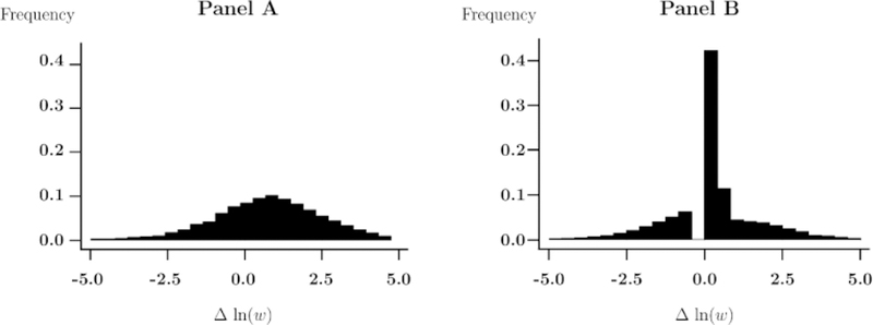
A simulated distribution of log-wage changes from the model for cases of no loss aversion (Panel A: λ = 1) and loss aversion (Panel B: λ = 2, a typical value in the literature) with the reference transaction in the steady-state case. Inflation is set equal to 1.6%: P/P₀ = 1.016. Real prices, wages, and the price level at the beginning of the year are normalized to 1: p₀ = w₀ = P₀ = 1. Model parameters are: ln(p) ~ N(0,1), c(e) = e²/4, σ = 0.8, μ_D = 1, and μ_A = 0.5. The firm and worker are assumed to always transact, regardless of the price realization, as long as the wage is positive. The number of simulation runs (including those dropped due to a negative wage) is 10,000. The width of each bin is 0.43.

Source: Author’s calculations.

It is sometimes argued that inflation “greases the wheels” of the labor market by enabling downward real wage adjustments to occur when it is eff cient for them to occur. In terms of the model, the nominal analog of Proposition 5 indeed implies that the real wage is downward flexible as long as the nominal wage does not need to be cut. However, the model also implies that inflation causes redistribution from workers to firms: because effort responds to the nominal wage, whenever the price level increases, the firm can induce its desired level of effort with a lower real wage.¹⁵ However, since a fall in the real wage reduces the worker’s material payoff, this redistribution will ultimately be limited by the firm’s need to beat the worker’s outside option. The model similarly predicts that deflation causes redistribution from firms to workers because when the price level falls, firms need to pay a higher real wage to induce any given level of effort.

The model also has implications for how the frequency distribution of wage changes depends on the average rate of increase of nominal prices Pp across firms. Starting from an average rate of increase close to zero, a higher rate—corresponding to an economy with a higher rate of inflation or productivity growth, or an industry experiencing growing demand—is predicted to generate a lower frequency of zero wage changes. A lower fraction of firms will be in the recent-decrease case, and hence a greater fraction of firms need to be hit by a negative shock in order to exhibit DNWR. Moreover, fewer firms will be hit by negative shocks. Consequently, fewer firms will be in the region of wage rigidity. Consistent with this prediction, Fehr and Goette’s (2005) evidence from Switzerland during 1991–1997 indicates that the frequency of zero nominal wage changes was lower in the early period of substantially higher inflation.

If most firms are experiencing sustained declines in Pp—as would occur in an economic environment of deflation or productivity decline, or an industry with contracting demand—then there will be very few zero wage changes because most firms will be in the recent-decrease case and thus wages will not be rigid when Pp falls. Consistent with this prediction, Kuroda and Yamamoto’s (2005) examination of wage changes in Japan suggests that there was DWNR during 1996–1997 at the beginning of the deflation, but wages have been downward flexible since 1998.

7. Efficiency of the Employment Transaction

Whereas the previous sections of this paper were primarily concerned with positive implications of the fairness model, this section discusses some normative implications. Because the wage is set in order to influence the worker’s effort rather than to clear the labor market, the model is an “efficiency wage” model. It therefore raises the same normative issues for the labor market as a whole regarding unemployment as other efficiency-wage models. In this section, I focus attention on normative questions regarding the efficiency of the bilateral transaction between the firm and the worker. To minimize notation, the formal analysis is restricted to the single-period version of the game from Section 5 (i.e., without money illusion).

Following Benjamin (2014), I distinguish between two notions of efficiency for studying interactions when agents have other-regarding preferences. “Material Pareto efficiency” is Pareto efficiency with respect to the purely self-regarding component of preferences (the worker’s material payoff and the firm’s profit), whereas “utility Pareto efficiency” is Pareto efficiency with respect to the overall objective function that the players maximize. In the present context, a transaction (w, e) is called material Pareto efficient (MPE) if there is no alternative transaction (w′,e′) such that u (w′,e′) ≥ u (w, e) and π (w′,e′) ≥ π (w,e), at least one inequality strict. A transaction (w,e) is called utility Pareto efficient (UPE) if there is no alternative transaction (w′,e′) such that U (w′, e′) ≥ U (w, e) and π (w′, e′) ≥ π (w, e), at least one inequality strict. I defer until later in this section a discussion of whether MPE or UPE may be the right social welfare criterion. I focus first on characterizing under what conditions the equilibria described in previous sections are MPE or UPE.

A transaction is MPE if and only if $\frac{\partial u(w,e)/\partial w}{\partial u(w,e)/\partial e}=\frac{\partial \pi (w,e)/\partial w}{\partial \pi (w,e)/\partial e}.$ Because the worker’s material payoff function and the firm’s profit are quasi-linear in the wage, this equality is equivalent to the worker exerting the efficient level of effort, e_eff (p); the wage does not matter for material efficiency because it is merely a transfer between profit and the worker’s material payoff. Thus, Proposition 1 immediately implies that in the absence of loss aversion, the equilibrium is MPE.

Proposition 6 shows that, in the absence of loss aversion, the equilibrium is also UPE.

Proposition 6.

Under Assumptions A and B, if the worker is not loss averse (λ = 1), then for any p > 1, the equilibrium transaction is UPE and MPE.

Proposition 6 follows immediately from Proposition 1 and Benjamin’s (2014) Theorem 1. To understand why the equilibrium is UPE, first notice that any UPE transaction must maximize the sum of surpluses because otherwise it would be utility-Pareto-dominated by an alternative transaction that maximized the sum of surpluses, had a higher wage and higher effort, and were at least as fair. Among the transactions that maximize the sum of surpluses, relative to the equilibrium, the firm would clearly be worse off if the wage were higher, and the worker would be worse off if the wage were lower since his material payoff would be lower and the transaction would be less fair.

The conclusion that the equilibrium is both MPE and UPE can be extended straightforwardly to apply also to the equilibrium of the dynamic game described in Proposition 3. Thus, in the absence of loss aversion, gift exchange that is sustained by fairness concerns can be eff cient regardless of which eff ciency notion is used.

This conclusion no longer holds if the worker is loss averse (λ > 1). The equilibrium is still UPE outside the ranges of wage and effort rigidity—and is MPE only when wage and effort remain unchanged from the previous period.

Proposition 7.

Under Assumption A, if the worker is loss averse (λ > 1) and the firm hires the worker in equilibrium, then the equilibrium transaction is UPE if and only if $p\notin ({\underset{\_}{p}}_{\text{W}-\text{rigid}},{\overline{p}}_{\text{W}-\text{rigid}})\cup ({\underset{\_}{p}}_{\text{e}-\text{rigid}},{\overline{p}}_{\text{e}-\text{rigid}}).$ The equilibrium transaction is also MPE if and only if $p={\overline{p}}_{\text{W}-\text{rigid}},$ or equivalently, if and only if the equilibrium transaction (w*,e*) satisfies w* = w₀ and e* = e₀.

Outside the ranges of wage and effort rigidity, the logic for why the equilibrium is UPE is similar to the non-loss-averse case. However, if the price realization occurs in $({\underset{\_}{p}}_{\text{W}-\text{rigid}},{\overline{p}}_{\text{W}-\text{rigid}}),$ then there is a utility-Pareto improvement: a small reduction in wage and effort that keeps profit constant. Because effort is inefficiently high (e* > e_eff (p)) in the region of wage rigidity, the joint reduction in wage and effort would increase the worker’s material payoff and (since profit is held constant) therefore also utility. Similarly, if the price realization occurs in $({\underset{\_}{p}}_{\text{e}-\text{rigid}},{\overline{p}}_{\text{e}-\text{rigid}}),$ then there is a utility-Pareto improvement. In this case, because effort is inefficiently low (e* < e_eff (p)), a joint, small increase in wage and effort that keeps profit constant would increase utility.

Turning to MPE, as noted at the beginning of Section 5.2, the equilibrium level of effort may not be e_eff (p)—and thus the equilibrium transaction may not be MPE. In fact, Proposition 5 implies that the equilibrium effort is the effcient level of effort only for the unique price realization at which w* = w₀ and e* = e₀. In the region of wage rigidity, effort is above the efficient level, and in the region of effort rigidity, effort is below it. For any other price realization, either (a) w* > w₀ and e* > e₀, or (b) w* < w₀ and e* < e₀. In case (a), the worker suffers a loss in effort but not wage, and therefore as noted at the beginning of Section 5.2, the equilibrium effort satisfies p = λc′ (e*) and hence is below the efficient level. In case (b), the worker suffers a loss in wage but not effort, and therefore the equilibrium effort satisfies $p=\frac{c^{\prime }\left(e^{*}\right)}{\lambda }$ and is above the efficient level.

Is UPE or MPE the more appropriate generalization of Pareto eff ciency to use as a welfare criterion? UPE is the appropriate generalization if the worker’s utility represents his “true” preferences, by which I mean what he would choose given correct beliefs and after deliberation. But there are a number of reasons why the worker’s behavior—as represented by his utility function—may deviate from his true preferences (for related discussion, see Benjamin 2014, Köszegi and Rabin 2008, and Sen 1973).

In the gift-exchange game studied here, one key question is whether the worker’s fair-minded behavior reflects his true preferences, or whether it reflects social norms or reliance on a heuristic (modeled in a reduced-form way via the utility specification) that he would reject upon further deliberation. For example, aiming to share total surplus equally may be a heuristic that he would endorse upon deliberation when interacting with another person but not when interacting with a firm. If the worker’s true preference when interacting with a firm coincided with his material payoff, then MPE would be the appropriate generalization of Pareto eff ciency.

Even if the worker’s fair-minded behavior is a true preference, his loss aversion may be at least partially a mistake. For example, loss aversion might reflect an immediate emotional reaction that would fade with deliberation. Even if the worker, upon deliberation, would choose to avoid current feelings of loss aversion, he might excessively choose to avoid losses under the mistaken belief that his current feelings of loss will persist (Loewenstein, O’Donoghue, and Rabin 2003). If loss aversion in this context is entirely an error, then the appropriate notion of effciency is UPE but with the worker’s utility calculated without loss aversion.¹⁶ (Money illusion is surely an error, even for a worker who truly has loss-averse preferences.)

In my view, theoretical reasoning alone cannot resolve the question of what are the worker’s “true” preferences—and indeed the answer may differ from one worker to another. The purpose of the analysis here is to highlight when and how the answer matters. To shed light on which preferences should be used for normative purposes, I believe that empirical evidence must also come into play (for related discussion, see Beshears et al 2008). For example, experimental research could examine whether and to what extent information or deliberation weaken loss aversion and fair-minded behavior. The conclusions from such research could be useful far beyond the specific analysis of the firm-worker interaction studied in this paper.

8. Concluding Remarks

The model of fairness concerns explored in this paper—a desire to equalize surplus payoffs judged relative to a reference transaction, which is determined by recent personal experience—also may explain a wide variety of observations about non-labor markets. For example, consumers may wish to punish firms that they believe are trying to extract more surplus from them than usual. Consistent with this hypothesis, during temporary periods of high demand, firms often voluntarily maintain prices below the market-clearing level, leading to long lines or stockouts (e.g., Rotemberg 2005, Olmstead and Rhode 1985, Dacy and Kunreuther 1969). Similarly, when costs increase, firms typically postpone raising prices. If it becomes clear that the cost increase is permanent and firms eventually raise their prices, firms often expend resources to inform customers that their profits have taken a hit. In housing markets, rent increases on new tenants are much more common than rent increases on existing tenants (Genesove 1999, Kahneman, Knetsch, and Thaler 1986).

The model explored in this paper is purposefully kept as simple as possible in order to make transparent the link between the worker’s fairness concerns and the model’s empirical implications. However, it is also important to examine more realistic models to investigate to what extent the conclusions from the simple model can be generalized.

Throughout the analysis, I have assumed that only workers have a concern for fairness. Results would be similar if firms have an analogous concern for fairness (see Benjamin 2014)—at least if the worker and the firm share the same reference transaction. In fact, however, disagreements about the reference transaction can be important in real-world interactions (indeed, Hart and Moore (2008) argue that the potential for such disagreements is a major motivation for contracting). For example, when there are several reasonable precedents, negotiators seem able to convince themselves that the one most favorable to themselves is the most relevant. This self-serving bias can often cause negotiations to break down (Babcock and Loewenstein 1997). Similar problems could arise if only one party has fairness preferences, but the selfish party does not know what the fair-minded party considers to be the reference transaction.

It would be useful to relax some of the restrictions from Assumption A. As noted in Section 3, if the worker is allowed to have a weaker dislike of advantageous unfairness, then results in the one-period model would be qualitatively similar, except that the equilibrium transaction would not be MPE. Allowing the worker to have a weaker dislike of disadvantageous unfairness can lead to a qualitatively different outcome, in which the firm exploits the worker’s willingness to altruistically provide effort.

Another valuable extension would be to embed the interaction between the firm and the worker in a labor market, in which the players’ outside options are determined by the prospects of finding another match. Such a model would make it possible to study how aggregate shocks affect aggregate wages and unemployment when workers’ loss aversion generates DNWR. Eliaz and Spiegler (2014) make progress in this direction.

Other important extensions include allowing the firm to be uncertain about the workers’ preferences (see footnote 1) and making the worker’s effort partially contractible. There has been some progress on both of these fronts in closely related models (e.g., Fehr, Klein, and Schmidt 2007).

References

- [1].Abowd John M. and Card David. Intertemporal labor supply and long-term employment contracts. American Economic Review, 77(1):50–68, March 1987. [Google Scholar]
- [2].Abowd John M., Kramarz Francis, and Margolis David N. High wage workers and high wage firms. Econometrica, 67(2):251–333, March 1999. [Google Scholar]
- [3].Agell Jonas and Lundborg Per. Theories of pay and unemployment: Survey evidence from swedish manufacturing firms. Scandinavian Journal of Economics, 97:295–307, 1995. [Google Scholar]
- [4].Akerlof George A., Dickens William T., and Perry George L. The macroeconomcis of low inflation. Brookings Papers on Economic Activity, (1):1–76, 1996. [Google Scholar]
- [5].Akerlof George A. and Yellen Janet L. The fair wage-effort hypothesis and unemployment. Quarterly Journal of Economics, 105(2):255–283, May 1990. [Google Scholar]
- [6].Andreoni James and B. Douglas Bernheim. Social image and the 50–50 norm: A theoretical and experimental analysis of audience effects. Econometrica, 77(5):1607–1636, 2009. [Google Scholar]
- [7].Babcock Linda and Loewenstein George. Explaining bargaining impasse: The role of self-serving biases. Journal of Economic Perspectives, 11(1):109–126, 1997. [Google Scholar]
- [8].Baker George, Gibbs Michael, and Holmstrom Bengt. The internal economics of the firm: Evidence from personnel data. Quarterly Journal of Economics, 109(4):881–919, November 1994. [Google Scholar]
- [9].Baker George, Gibbs Michael, and Holmstrom Bengt. The wage policy of a firm. Quarterly Journal of Economics, 109(4):921–955, November 1994. [Google Scholar]
- [10].Ball Laurence and N. Gregory Mankiw. Asymmetric price adjustment and economic fluctuations. Economic Journal, 104(423):247–261, March 1994. [Google Scholar]
- [11].Beaudry Paul and DiNardo John. The effect of implicit contracts on the movement of wages over the business cycle: Evidence from micro data. Journal of Political Economy, 99(4):665–688, August 1991. [Google Scholar]
- [12].Benjamin Daniel J. A theory of fairness in labor markets. Harvard University mimeo, November 2005. [Google Scholar]
- [13].Benjamin Daniel J. Distributional preferences, reciprocity-like behavior, and efficiency in bilateral exchange. American Economic Journal: Microeconomics, Forthcoming. [DOI] [PMC free article] [PubMed] [Google Scholar]
- [14].Beshears John, Choi James J., Laibson David, and Madrian Brigitte C. How are preferences revealed? Journal of Public Economics, 92(8–9):1787–1794, 2005. [DOI] [PMC free article] [PubMed] [Google Scholar]
- [15].Bewley Truman F. Why Wages Don’t Fall During a Recession. Harvard University Press, Cambridge, MA, 1999. [Google Scholar]
- [16].Bils Mark J. Real wages over the business cycle: Evidence from panel data. Journal of Political Economy, 93:666–689, 1985. [Google Scholar]
- [17].Blinder Alan S. and Choi Don H. A shred of evidence on theories of wage stickiness. Quarterly Journal of Economics, 105(4):1003–1015, November 1990. [Google Scholar]
- [18].Bolton Lisa E., Warlop Luk, and Alba Joseph W. Explorations in price (un)fairness. Journal of Consumer Research, 29:474–91, March 2003. [Google Scholar]
- [19].Brown Martin, Falk Armin, and Fehr Ernst. Relational contracts and the nature of market interactions. Econometrica, 72(3):747–780, May 2004. [Google Scholar]
- [20].Campbell Carl M. III and Kamlani Kunal S. The reasons for wage rigidity: Evidence from a survey of firms. Quarterly Journal of Economics, 112(3):759–789, August 1997. [Google Scholar]
- [21].Card David, Mas Alexandre, Moretti Enrico, and Saez Emmanuel. Inequality at work: The effect of peer salaries on job satisfaction. American Economic Review, 102(6):2981–3003, 2012. [Google Scholar]
- [22].Charness Gary and Kuhn Peter. Does pay inequality affect worker effort? experimental evidence. Journal of Labor Economics, 25(4):693–723, 2007. [Google Scholar]
- [23].Charness Gary and Rabin Matthew. Understanding social preferences with simple tests. Quarterly Journal of Economics, 117(3):817–869, August 2002. [Google Scholar]
- [24].Cohn Alain, Fehr Ernst, and Goette Lorenz. Fair wages and effort provision: Combining evidence from the lab and the field. 2013. University of Zurich Department of Economics Working Paper Series No. 107. [Google Scholar]
- [25].Collard Fabrice and la Croix David de. Gift exchange and the business cycle: The fair wage strikes back. Review of Economic Dynamics, 3:166–193, 2000. [Google Scholar]
- [26].Dacy DC and Kunreuther H The economics of natural disasters. Free Press, New York, 1969. [Google Scholar]
- [27].Devereux Paul J. The importance of obtaining a high paying job. 2002. UCLA Working Paper. [Google Scholar]
- [28].Dickens William T., Goette Lorenz, Groshen Erica L., Holden Steinar, Messina Julian, Schweitzer Mark E., Turunen Jarkko, and Ward Melanie E. How wages change: Micro evidence from the international wage flexibility project. Journal of Economic Perspectives, 21(2):195–214, 2007. [Google Scholar]
- [29].Dickens William T. and Katz Lawrence F. Inter-industry wage differences and theories of wage determination. NBER Working Paper No. 2271, June 1987. [Google Scholar]
- [30].Doeringer Peter B. and Piore Michael J. Internal Labor Markets and Manpower Analysis. D.C. Heath and Company, Lexington, MA, 1971. [Google Scholar]
- [31].Ehrenberg Ronald G. and Milkovich George T. Compensation and firm performance. NBER Working Paper No. 2145, February 1987. [Google Scholar]
- [32].Eliaz Kfir and Spiegler Ran. Reference dependence and labor market fluctuations In Parker Jonathan A. and Woodford Michael, editors, NBER Macroeconomics Annual 2013, pages 159–200. University of Chicago Press, 2014. [Google Scholar]
- [33].Elsby Michael W. L. Evaluating the economic significance of downward nominal wage rigidity. August 2004. Working paper. [Google Scholar]
- [34].Elsby Michael W. L. Evaluating the economic significance of downward nominal wage rigidity. Journal of Monetary Economics, 56(2):154–169, 2009. [Google Scholar]
- [35].Constanca Esteves-Sorenson and Rosario Macera. Revisiting gift exchange: Theoretical considerations and a field test. 2013. Yale University Working Paper. [Google Scholar]
- [36].Constanca Esteves-Sorenson, Rosario Macera, and Robert Broce. Do monetary incentives crowd out intrinsic motivation? a field test in the workplace. August 2014. Yale University Working Paper. [Google Scholar]
- [37].Fehr Ernst and Falk Armin. Wage rigidity in a competitive incomplete contract market. Journal of Political Economy, 107:106–134, 1999. [Google Scholar]
- [38].Fehr Ernst and Goette Lorenz. Robustness and real consequences of nominal wage rigidity. Journal of Monetary Economics, 52:779–804, 2005. [Google Scholar]
- [39].Fehr Ernst, Goette Lorenz, and Zehnder Christian. A behavioral account of the labor market: The role of fairness concerns. Annual Review of Economics, 1:355–84, 2009. [Google Scholar]
- [40].Fehr Ernst, Kirchsteiger Georg, and Riedl Arno. Does fairness prevent market clearing? an experimental investigation. Quarterly Journal of Economics, 108(2):437–459, 1993. [Google Scholar]
- [41].Fehr Ernst, Kirchsteiger Georg, and Riedl Arno. Gift exchange and reciprocity in competitive experimental markets. European Economic Review, 42:1–34, 1998.12321972 [Google Scholar]
- [42].Fehr Ernst, Klein Alexander, and Schmidt Klaus M. Fairness and contract design. Econometrica, 75(1):121–154, 2007. [Google Scholar]
- [43].Fehr Ernst and Schmidt Klaus M. A theory of fairness, competition, and cooperation. Quarterly Journal of Economics, 114(3):817–868, August 1999. [Google Scholar]
- [44].Friedman Milton. The role of monetary policy. American Economic Review, 68:1–17, March 1968. [Google Scholar]
- [45].Genesove David. The nominal rigidity of apartment rents. NBER Working Paper No. 7137, May 1999. [Google Scholar]
- [46].Gneezy Uri and List John. Putting behavioral economics to work: Field evidence on gift exchange. Econometrica, 74(5):1365–1384, 2006. [Google Scholar]
- [47].Grant Darren. The effect of implicit contracts on the movement of wages over the business cycle: Evidence from the national longitudinal surveys. Industrial and Labor Relations Review, 56(3):393–408, April 2003. [Google Scholar]
- [48].Greenberg Jerald. Employee theft as a reaction to underpayment inequity: The hidden cost of pay cuts. Journal of Applied Psychology, 75(5):561–568, 1990. [Google Scholar]
- [49].Gregory Gregory N Macroeconomics. Worth Publishers, New York, NY, 1994. [Google Scholar]
- [50].Harris Milton and Holmstrom Bengt. A theory of wage dynamics. Review of Economic Studies, 49(3):315–333, July 1982. [Google Scholar]
- [51].Hart Oliver and Moore John. Contracts as reference points. Quarterly Journal of Economics, 123(1):1–48, February 2008. [Google Scholar]
- [52].Heike Hennig-Schmidt Abdolkarim Sadrieh, and Rockenbach Bettina. In search of workers’ real effort reciprocity–a field and a laboratory experiment. Journal of the European Economic Association, 8(4):817–837, 2010. [Google Scholar]
- [53].Herz Holger and Taubinsky Dmitry. Market experience is a reference point in judgments of fairness. 2013. University of Zurich, Department of Economics Working Paper No. 128. [Google Scholar]
- [54].Kahn Lisa. The long-term labor market consequences of graduating from college in a bad economy. Labour Economics, 17(2):303–316, 2010. [Google Scholar]
- [55].Kahneman Daniel, Knetsch Jack L., and Thaler Richard H. Fairness as a constraint on profit seeking entitlements in the market. American Economic Review, 76(4):728–41, 1986. [Google Scholar]
- [56].Kahneman Daniel and Tversky Amos. Prospect theory: An analysis of decision under risk. Econometrica, 47(2):263–91, 1979. [Google Scholar]
- [57].Kaufman Roger T. On wage stickiness in britain’s competitive sector. British Journal of Industrial Relations, 22:101–12, 1984. [Google Scholar]
- [58].Koszegi Botond and Rabin Matthew. A model of reference-dependent preferences. Quarterly Journal of Economics, 121(4):1133–1166, 2006. [Google Scholar]
- [59].Koszegi Botond and Rabin Matthew. Choices, situations, and happiness. Journal of Public Economics, 92:1821–1832, 2008. [Google Scholar]
- [60].Kruse David. Does profit sharing affect productivity? NBER Working Paper No. 4–54-2, November 1993. [Google Scholar]
- [61].Kruse Douglas, Freeman Richard, Blasi Joseph, Buchele Robert, Scharf Adrin, Rodgers Loren, and Mackin Chris. Motivating employee-owners in esop firms: Human resource policies and company performance. NBER Working Paper No. 10177, December 2003. [Google Scholar]
- [62].Kube Sebastian, Puppe Clemens, and Mar’e9chal Michel. Do wage cuts damage work morale? evidence from a natural field experiment. Journal of the European Economic Association, 11:853–870, 2013. [Google Scholar]
- [63].Kuroda Sachiko and Yamamoto Isamu. Wage fluctuations in japan after the bursting of the bubble economy: Downward nominal wage rigidity, payroll, and the unemployment rate. Monetary and Economic Studies, 23(2):1–30, 2005. [Google Scholar]
- [64].Lee Darin and Rupp Nicholas G. Retracting a gift: How does employee effort respond to wage reductions? Journal of Labor Economics, 25(4):725–761, 2007. [Google Scholar]
- [65].Levine David I. Fairness, markets, and ability to pay: Evidence from compensation executives. American Economic Review, 83(5):1241–1259, December 1993. [Google Scholar]
- [66].Loewenstein George, Ted O’Donoghue, and Matthew Rabin. Projection bias in predicting future utility. Quarterly Journal of Economics, 118(4):1209–1248, 2003. [Google Scholar]
- [67].MacLeod B and Malcolmson JM Implicit contracts, incentive compatibility, and involuntary unemployment. Econometrica, 57:312–22, 1989. [Google Scholar]
- [68].Mas Alexandre. Pay, reference points, and police performance. Quarterly Journal of Economics, 121, 2006. [Google Scholar]
- [69].Mathewson Stanley B. Restriction of Output Among Unorganized Workers. Southern Illinois University Press, Carbondale, IL, 2nd edition, 1969. [Google Scholar]
- [70].Maximiano Sandra, Sloof Randolph, and Sonnemans Joep. Gift exchange in a multi-worker firm. Economic Journal, 117:1025–1050, 2007. [Google Scholar]
- [71].Olmstead AL and Rhode P Rationing without government: The west coast gas famine of 1920. American Economic Review, 75:1044–55, 1985. [Google Scholar]
- [72].Prendergast Canice. The provision of incentives in firms. Journal of Economic Literature, 37(1):7–63, March 1999. [Google Scholar]
- [73].Pritchard Robert D., Dunnette Marvin D., and Jorgenson Dale O. Effects of perceptions of equity and inequity on worker performance and satisfaction. Journal of Applied Psychology, 56(1):75–94, 1972. [Google Scholar]
- [74].Rabin Matthew. Incorporating fairness into game theory and economics. American Economic Review, 83(5):1281–1302, December 1993. [Google Scholar]
- [75].Rees-Jones Alex. Loss aversion motivates tax sheltering: Evidence from u.s. tax returns. December 2014. Wharton Working Paper. [Google Scholar]
- [76].Rotemberg Julio J. Fair pricing. March 2005. Harvard Business School mimeo. [Google Scholar]
- [77].Seltzer Andrew and Merrett David. Personnel policies at the union bank of australia: Evidence from the 1888–1900 entry cohorts. Journal of Labor Economics, 18(4):573–613, October 2000. [Google Scholar]
- [78].Sen Amartya. Behaviour and the concept of preference. Economica, 40(159):241–259, 1973. [Google Scholar]
- [79].Shafir Eldar, Diamond Peter, and Tversky Amos. Money illusion. Quarterly Journal of Economics, 112(2):341–74, 1997. [Google Scholar]
- [80].Solon Gary, Barsky Robert, and Parker Jonathan A. Measuring the cyclicality of real wages: How important is composition bias? Quarterly Journal of Economics, 109(1):1–25, 1994. [Google Scholar]
- [81].Thaler Richard. Mental accounting and consumer choice. Marketing Science, 4(3):199–214, 1985. [Google Scholar]
- [82].Tobin James. Inflation and unemployment. American Economic Review, 62(½):1–18, March 1972. [Google Scholar]
- [83].Elaine Walster G William Walster, and Ellen Berscheid Equity: Theory and Research. Allyn and Bacon, Boston, 1977. [Google Scholar]
- [84].Weitzman Martin L. and Kruse Douglas. Profit sharing and productivity In Blinder Alan, editor, Paying for Productivity. Brookings Institution, Washington, D.C., 1990. [Google Scholar]