

Abstract
While tomographic imaging of cardiac structure and kinetics has improved substantially, electrophysiological mapping of the heart is still restricted to the surface with little or no depth information beneath. The progress in reconstructing 3-D action potential from surface voltage data has been hindered by the intrinsic ill-posedness of the problem and the lack of a unique solution in the absence of prior assumptions. In this work, we propose a novel adaption of the total-variation (TV) prior to exploit the unique spatial property of transmural action potential of being piecewise smooth with a steep boundary (gradient) separating depolarized and repolarized regions. We present a variational TV-prior instead of a common discrete TV-prior for improved robustness to mesh resolution, and solve the TV-minimization by a sequence of weighted, first-order L2-norm minimization. In a large set of phantom experiments, the proposed method is shown to outperform existing quadratic methods in preserving the steep gradient of action potential along the border of infarcts, as well as in capturing the disruption to the normal path of electrical wavefronts. Real-data experiments also further demonstrate the potential of the proposed method in revealing the location and shape of infarcts when quadratic methods fail to do so.
Keywords: Inverse problem of electrocardiography, myocardial ischemia and infarction, noninvasive transmural electrophysiological imaging, total-variation minimization
I. Introduction
HEART disease is one of the leading causes of death worldwide since the 1970s [1]. Because the heart is an electromechanically coupled organ, its efficient contraction must be preceded by coordinated and steady electrical excitation spreading three-dimensionally throughout the myocardium. Disruptions to this electrical propagation can directly predispose the heart to mechanical catastrophe and lead to sudden cardiac death. However, while methods for noninvasive imaging and analysis of 3-D structure [2], kinetics [3], and mechanics [4] of an individual’s heart have substantially improved in recent years, methods for assessing the electrophysiological (EP) aspects have not. In practice, common observations of cardiac electrical activity are voltage data either sensed on the body-surface as noninvasive electrocardiograms (ECG) or mapped on the heart surface by catheters introduced into the cavity in an invasive manner. Other limitations aside (e.g., the complexity and cost of an invasive procedure), both types of data only provide a surface surrogate for intramural electrical activity that occurs deep beneath the surface of the heart [5]. This lack of information has not only limited our understanding of electrical and electromechanical mechanism of many heart diseases, but also prevented the development of diagnostic and therapeutic tools to their full potential.
The critical gap in experimental methods has motivated many computational methods for noninvasive EP imaging that, analogous to tomographic imaging, solve an inverse problem to quantitatively reconstruct transmural action potential from body-surface voltage data. The forward relationship between the current source in the heart and the bioelectric field (most commonly measured in the body surface by ECG) is governed by the quasi-static equation of electromagnetism theory [6]. Unfortunately, this inverse problem is plagued by two types of ill-posedness: 1) the mathematical ill-posedness caused by the limited number of measurements, i.e., the dimension of measurements is typically much smaller than the dimension of unknown variables; and 2) the physical ill-posedness decided by the Helmholtz’s equivalent double-layer principle of electromagnetic field, i.e., an infinite number of intramural solutions fit the same electrical field on the surface [6].
In exchange for a unique solution, a common assumption in existing approaches to electrophysiological imaging restricts the solutions to the surface of the heart, represented by the reconstruction of epicardial potential [7], [8] and the reconstruction of activation/recovery time on both the epicardium and endocardium [9], [10]. Various regularization methods have been applied to reduce the mathematical ill-posedness of electrophysiological inverse problem. For instance, the commonly used Tikhonov regularization (zero-order, first-order, second-order) [11], truncated-SVD [12], [13], and state-space filtering framework (Kalman filter) [14] have been used to reconstruct the heart surface potential with minimum overall energy while producing body-surface potential field consistent with the measurements. Although these regularization methods lead to an efficient linear inverse operator, the solutions are often smooth. Recently, L1-norm-based regularization was proposed to improve the resolution of the reconstructed heart surface potential [15], [16].
Over the past decades, transition to intramural EP imaging has been limited due to the challenge of nonunique solutions associated with the intramural solution. Existing approaches can be generally divided into two classes. One is to directly regularize the intramural EP reconstruction with a different order of smoothness constraints imposed on the spatial and/or temporal properties of the solution [17]–[19]. As the solution space increases and the physically-induced nonuniqueness appears with a transmural solution, additional constraints may be needed in order to guarantee unique, meaningful solutions for these approaches. Alternatively, a 3-D computational model of whole-heart excitation can be introduced to guide the inverse problem either in a deterministic optimization [20] or statistical inference [5]. While allowing the inclusion of additional prior knowledge about the electrophysiology and biophysics of the heart, these approaches may be subject to the influence of these a priori physiological assumptions when they differ substantially from real individual conditions.
The proposed work is based on the fundamental hypothesis that, while L2-based quadratic regularization is suitable for alleviating the mathematical ill-posedness of the problem caused by limited data, L1-based sparse regularization is further needed for resolving the nonuniqueness of the solution. In particular, we propose to view the transmural action potential u(t) as a time-varying 3-D image. As illustrated in Fig. 1, the edge of this image [i.e., spatial gradient ∇u(t)] is always localized and steep in space. During the depolarization and repolarization, it represents the steep wavefront between active and resting regions [Fig. 1(a)], revealing alterations in the normal electrical excitation in diseased hearts. Between the two phases (the ST and UP segment of an ECG cycle), ∇u(t) is expected to be close to zero everywhere in a normal heart, and an appearance of high gradient would indicate underlying pathology, such as the border of a region of ischemic tissue [Fig. 1(b)]. Thus, it is important to preserve the unique spatial feature of ∇u(t) during the reconstruction of u(t), and this can be accomplished by total-variation (TV) minimization, which promotes a solution with sharp boundaries/gradients between piecewise smooth regions [21].
Fig. 1.

Illustration of the 3-D action potential and its spatial gradient in (a) a normal heart and (b) an infarcted heart.
Since its original development, TV-minimization has been applied to preserve the sharp edge of an image in a variety of image-processing and computer-vision applications such as image de-noising [22], blind de-convolution [23], and inpainting [24]. Most of these existing applications deal exclusively with regular grids of pixels or voxels and, correspondingly, the discrete TV prior is commonly defined as the L1-norm of the gradient field of the grid. In comparison, the biophysical application targeted in this paper involves a complex volumetric mesh of heart geometry, which is discretized with an unstructured grid. It therefore faces the following unique challenges: 1) the commonly used discrete definition of TV-prior—based on the gradient field of the discrete mesh—is highly affected by the resolution of the discrete mesh; and 2) the gradient of the discrete mesh—given its complex shape and unstructured node distribution—is much more difficult and error-prone to calculate than that of a digital image.
In this paper we propose a novel adaptation of the spatial TV-prior into transmural EP imaging that will overcome the challenge associated with TV-minimization on a complex, unstructured mesh. First, to ensure the accuracy of TV calculation on an irregular cardiac mesh and to improve its robustness to the resolution of this discrete mesh, we introduce a variational TV-prior to approximate the continuous TV-prior by a numerical integration. Second, adapting the concept from iteratively reweighted least-square approximation of L1-minimization [25], an iterative algorithm is developed to solve the TV-minimization by a sequence of weighted, first-order L2-minimizations where the weight changes in each iteration. Finally, we consider the combination of the TV-prior with a L2-based (minimum-square-error in data fitting) and a L1-based data-fidelity terms (minimum-absolute-error in data fitting) and compare their performance in terms of robustness to measurement noises and computational cost. In the complete form of the algorithm, a simple quadratic regularization is first used to overcome the mathematical ill-posedness of the reconstruction problem and to initialize the proposed TV-minimization. The proposed iteratively reweighted method then prunes the initially diffused solution and overcomes the challenge of physically-induced nonunique solutions.
Evaluation of the presented method is carried out in two different application settings. Primarily, to systematically evaluate the potential of the presented method in detecting and preserving the steep gradient of action potential distributed along the border of an ischemic or infarcted region (during the ST-segment of an ECG cycle), a large set of phantom and real-data experiments is conducted. The former are simulated on four realistic heart–torso structures considering myocardial infarcted/ischemic regions of different locations and sizes within the left-ventricular (LV) wall. First, a comparison study involving 137 phantom experiments is done between the presented TV-minimization method and existing quadratic methods in intramural electrical reconstruction [18], [26]. The results show that the presented method delivers significantly higher accuracy (t-test) over quadratic approaches in localizing action potential gradient along ischemic regions. Second, a set of 60 experiments is carried out to show the higher accuracy, robustness, and computational efficiency of the proposed variational TV-prior in TV-minimization in comparison to a discrete TV-prior that is commonly used in image processing. Finally, a comparison study between L2-based and L1-based data-fidelity terms is conducted on 90 phantom experiments with six different levels of noises, showing that the use of an L1-based data fidelity is more robust and of faster convergence in the presence of high noise levels, while the L2-based data fidelity delivers higher accuracy at the presence of low to moderate measurement noises. Real-data experiments on two post-infarction patients further verify the potential of the proposed method in detecting the abnormally steep gradient along the infarct border. This ability to reveal the shape of the infarct is important for guiding interventional therapies such as catheter ablation [27].
In addition, initial phantom studies also are carried out to demonstrate the ability of the presented method in reconstructing and preserving the dynamic structure of excitation wavefronts during both normal and pathological conditions. It also is shown to outperform existing quadratic methods in preserving the structure of narrow wavefronts and in capturing the change of these wavefronts caused by the existence of infarct tissue. While TV-minimization has been adopted in recent works for improving the resolution of epicardium potential reconstruction [15], [16], the important difference and novelty here are that we are aiming at intramural reconstruction. The use of TV-minimization is not only motivated by the improvement of reconstruction resolution but, more importantly, is tied to the intrinsic spatial property of intramural action potential and the clinical significance of its gradient region (i.e., narrow wavefront, or abnormal value along ischemic/infarcted region).
II. Forward Problem of Electrocardiography
Cardiac electrical excitation produces time-varying voltage signals on the body surface; their generation can be described using quasi-static approximation of the electromagnetic theory. Within the myocardium volume Ωh, the bidomain theory [28] defines the distribution of the extracellular potential ϕte as a result of the gradients of action potential u, which is given
| (1) |
where r stands for the spatial coordinate, Di and De are the effective intracellular and extracellular conductivity tensors, and Dk = Di + De is bulk conductivity tensor.
In the region bounded between heart surface and the body surface, potentials ϕt are calculated assuming that no other active electrical source exists within the torso as
| (2) |
where Dt is the torso conductivity tensor and Ωt/h the entire thorax except Ωh.
Within the myocardium equation (1) applied, because the anisotropic ratio of Dk is a magnitude smaller than that of Di [28], we only retain the anisotropy of Di to reduce model complexity; therefore, Dk and Dt become scalars σk and σt. In the torso volume external to the heart equation (2), we assume homogeneous and isotropic conduction because it has been shown that torso conductivity modulates only the magnitude but not the pattern of body-surface signal [29]. Based on these assumptions, the forward relationship between cardiac action potential u(t) and body-surface voltage data ϕ(t) can be described in the following Poisson equation within the heart and Laplace equation external to the heart
| (3) |
| (4) |
In this study, (3) and (4) are solved with the coupled mesh-free and boundary element methods [29], [30]. The value of anisotropic intracellular conductivity tensor Di, bulk conductivity σk, and torso conductivity σt are adopted from [31]. This gives us a biophysical model on a subject-specific heart–torso model derived from tomographic images
| (5) |
where the transfer matrix H is specific to each individual’s torso anatomy and is typically considered time-invariant as the motion induced by heart contraction and relaxation process is disregarded. The condition number of H was shown to be typically at the order of 1016 [5].
III. Total-Variation Regularization for Transmural Electrophysiological Imaging
We propose to incorporate the TV-prior into the reconstruction of transmural action potential; at this stage, we exclude the temporal factor and focus on the reconstruction with a spatial TV-prior at separate time instants. Therefore, the estimation of transmural action potential from body-surface potential data can be formulated as
| (6) |
where g indicates L1 norm or L2 norm of data-fidelity term. TV(u) denotes the total-variation of u. For a continuous signal u, its total-variation is defined as [22]
| (7) |
The first challenge comes from defining a proper discretization of TV(u) that is close to its continuous definition in (7) regardless of the resolution of the unstructured volumetric mesh of the heart [Fig. 2(b)].
Fig. 2.

(a) Coupled heart-torso model with the torso represented by boundary elements. (b) Ventricular model represented by meshfree nodes. Surface mesh is provided for better visualization. (c) AHA 17-segment division of LV with three transmural layers.
A. Variational TV-Prior
In most image-processing applications, a discrete version of TV(u) is calculated as the L1-norm of the discrete gradient field of u
| (8) |
where n represents the total number of discrete points (usually pixels of an image).
With this definition, it is not possible to formulate an explicit gradient operator for the entire discrete field without separately employing directional gradient operator. One popular method is based on anisotropic separable approximation [32]
| (9) |
where horizontal-, vertical-, and depth-discrete derivative operators D are denoted by Dx, Dy, and Dz, respectively. Such approximation sacrifices accuracy for the simplicity of numerical maneuver and, more importantly, will introduce large matrix computation and storage during the optimization process a we will show in Section III-B. Individual elements in D, while straightforward to calculate in digital images because of the regular grid of pixels, are not trivial to calculate accurately when the nodes of the discrete mesh of u are distributed irregularly in space. Furthermore, this definition can differ substantially from the TV of the underlying continuous field in (7), depending on the resolution of u.
Therefore, we define an alternative approximation of the continuous form of TV as
| (10) |
where a numerical integration is performed over the 3-D myocardial field by N (at the order of 105) Gaussian quadrature points. Depending on the discretization method used (such as the finite element method or meshfree method [33] used in our study [29], [30]), ∇u on each Gauss point is approximated by a linear combination of its neighboring nodal points in the discrete field u based on the 3 × n spatial gradient of the shape function φi. Because each Gauss point has only a small set of support nodal points, φi and ∇φi are sparse with a small number of nonzero values. This definition of TV(u) does not directly rely on the discrete mesh of u; hence it is robust to the spatial resolution of u. Furthermore, it is also consistent with the data-fidelity term in (6), where the biophysical model H is also calculated from numerical approximations of integrals involved in the quasi-static Maxwell equations.
B. Iteratively Reweighted Minimization of TV (IRTV)
Once the L1-norm is applied to the constraint term, the corresponding term is difficult to be solve directly. In this study, we adopt the concept of iteratively re-weighted (IR) to handle this challenge. The general idea of IR is based on the following iterative approximation of each element x in vector x at iterate k [25]
| (11) |
namely, the L1-norm of x is approximated by the L2-norm of a weighted-x, where the weight is the square root value of the x obtained at the previous iteration. Because the value of x from the previous iteration is known, the L1 regularization problem can be approximated by a sequence of weighted L2 regularization with the weight changing at each iteration depending on the solution from the previous iteration.
Adopting the concept of IR, we can approximate the continuous form of TV as a sequence of L2-norm of weighted ∇u, each weight being the square root of ∇u at the previous (k–1)th iteration, i.e.,
| (12) |
Coupling this with our proposed variational approximation of TV using (10), (12) can be approximated again by variational approximation in weighted L2 form
| (13) |
where
| (14) |
In other words, at each iteration the proposed variational TV-prior is approximated by a weighted L2-norm of u, with the weight matrix WTW defined as above. It is important to note that, once a discrete mesh of the heart is constructed with Gaussian quadrature points established, shape functions used for calculating WTW remain fixed and the only change in WTW at each iteration comes from u(k–1). Therefore, at each iteration, computation of the weight matrix involves only weighting N pre-stored sparse matrices—one for each Gauss point—by a scalar ∣∇φiu∣ and adding them together.
For the sake of comparison, applying IR concept to (9), the L1-norm of the gradient field ∥∇u∥1 can also be approximated by weighted L2-norm. The weight matrix DTWdD is assembled from [25]
| (15) |
where the dimension of matrix D is 3n × n and the dimension ol Wd is 3n × 3n. It is evident that, by using the discrete TV form as defined in (9), the IRTV will involve a much larger weigh matrix that will substantially increase the computation of the iterative procedure. Comparison between these two approaches will be performed in phantom experiments [Section IV-A (2)].
C. IRTV-L2 Versus IRTV-L1
With the proper TV approximation determined, the next task is to determine the norm of the data-fidelity term in (6). Recent studies have shown that, when combined with an L1-norm regularization term, an L1-norm data fidelity shows higher robustness to measurement errors as well as faster convergence in comparison to an L2-based data-fidelity norm [8]. Recently renewed interest in sparse reconstruction also showed that L1-based error term is more suitable for handling outlines of salt-and-pepper-like errors where most of the measurements are correct with large errors in only a few locations [15]. In this study we will consider both IRTV-L2 and IRTV-L1 approaches in order to obtain a better understanding of their differences.
IRTV-L2:
First, we consider a common least-square data-fidelity term (setting q in (6) equal to 2). Based on the expanded IR concept in (13), the IRTV-L2 minimization can be solved by a set of weighted L2-minimizations
| (16) |
| (17) |
where λ(k) is the regularization parameter used at iteration k. is slightly modified from W in (14) so that a small positive value β is introduced to reduce numerical errors when ∣∇φiu(k–1)∣ at the ith Gauss point is close to zero.
In this way, by iteratively solving the L2 regularization, the local region with a small spatial gradient (being in the denominator) will generate a large penalty in the current iteration, while a large gradient will be promoted until the final solution exhibits a piecewise smooth pattern with steep gradient. The convergency of the solution of IR to the minimum of the original objective function was previously proved in [25].
IRTV-L1:
Second, we consider the alternative of a L1-norm data-fidelity term (setting q in (6) equal to 1). The concept of IR can be extended to this IRTV-L1 model by replacing the L1-norm data-fidelity term with a sequence of weighted L2-norm with the weight matrix at each iteration k defined by . Again, this IRTV-L1 problem can be solved as a sequence of weighted L2-minimizations
| (18) |
| (19) |
| Algorithm 1 Iteratively re-weighted minimization of Total-Variation (IRTV-Lq) | |
|
|
For both IRTV-L2 and IRTV-L1, matrix inversion is calculated by Conjugate Gradient method in this study.
D. Algorithm Summary
To put together the whole picture, we need to resolve two further issues.
Initialization:
The proposed TV method has to be initialized by a method that is able to overcome the mathematical illposedness using smoothness constraints. Here, the zeroth-order Tikhonov regularization is used for the initial solution of u(0).
Regularization Parameter:
For the initialization that uses Tikhonov regularization, λ(0) is calculated by the L-curve method [34]. After initialization, the iteration as described above (17) and (18) repeats until the convergence criterion, i.e., the difference between two successive gradients of solutions is smaller than a predefined tolerance. Unfortunately, there is currently no established method for objectively determining regularization parameter in L1-based problems, and most reports rely on an empirical and supervised procedure to select an optimal value of λ after a large set of experiments [35], [36]. In the proposed IRTV method, because the regularization term in the objective function changes in each iteration (as the weight of the L2-norm penalty changes), a less supervised approach for the selection of λ(k) is needed for a robust algorithm. Here, we adopt the method proposed in [37] to automatically update the magnitude of λ(k) at each iteration based on the infinity norm of the matrices involved in the data-fidelity and the regularization terms (see Algorithm 1 for the expression of λ(k)).
A complete summary of the algorithm for both the IRTV-L2 and IRTV-L1 is provided in Algorithm 1.
IV. Phantom Experiments
First, we evaluate the proposed method through phantom experiments conducted on four realistic human heart and torso models derived from axial 0.8–3.0 mm CT scans. Fig. 2(a) and (b) give one example where the homogeneous torso model is represented with boundary-element mesh and the 3-D ventricular model is represented with meshfree nodes [29], [30]. We focus on the ability of the proposed reconstruction method to: 1) outline the steep gradient of action potential Δu along the border of the infarcted or ischemic region that separates the region of necrotic/inactive and healthy/active tissue during the ST-segment of an ECG cycle, and 2) reconstruct the excitation wavefront in both normal and diseased hearts so as to reveal the underlying block (disease substrate) to the conduction path.
The accuracy of the proposed method is measured in two ways. Firstly, we define a consistency metric (CoM) to measure the accuracy of the region of detected steep gradients (10) by calculating the percentage of true positives in the sum of true positives, false positives, and true negatives
| (20) |
where S1 represents the region of steep gradients (in terms of the number of meshfree nodes) in the reconstructed action potentials and S2 is the region of steep gradients in the ground truth setting. In the current study, the region of steep gradients is outlined using a threshold value determined by mean(∇u) + 1/2* std(∇u), where mean(∇u) represents the mean of steep gradients of action potential and std(∇u) is standard deviation of steep gradients. Secondly, we also quantity the correlation coefficient (CC) between the true and reconstructed action potential
| (21) |
where the subscript “t” refers to the ground truth, “r” refers to the reconstructed action potential, and the bar “—” refers to the mean value.
A. Reconstruction Along Infarct Border
As explained in Section I, during the ST segment of an ECG cycle, the myocardium of healthy ventricles should all be depolarized and remaining at the plateau phase of an action potential cycle. Therefore, a minimal spatial gradient of action potential is expected. In the heart with myocardial infarction, however, the voltage difference between the region of depolarized healthy tissue and necrotic tissue produces a steep gradient bordering the 3-D region of infarct. Because the heterogeneity and morphology of infarct border zone has been recognized as one main substrate for lethal ventricular arrhythmias [27], the ability to preserve this gradient in the noninvasive reconstruction of action potential has the potential to help the pre-planning of interventional therapies such as catheter ablation of ventricular tachycardia.
In this set of phantom experiments, action potential during the ST-segment are set at 0 for the infarct core and 1 for the health region. Body-surface ECGs are simulated and Gaussian white noise with a signal-noise ratio (SNR) based on the signal energy, i.e., zero-mean Gaussian noise with a standard deviation calculated from SNR, is added as inputs for transmural reconstruction of action potential. Three groups of comparison studies are performed.
IRTV versus existing quadratic (L2) regularization-based methods for transmural EP reconstruction, including the first-order [18] and zeroth-order [26] Tikhonov regularization.
Variational TV-prior equation (13) versus discrete TV-prior equation (15) [25] as described in Section III-A.
IRTV-L1 versus IRTV-L2 as described in Section III-C.
1). IRTV Versus Existing Quadratic-Regularization:
In this set of phantom experiments, 370-lead body-surface ECG are simulated and corrupted with 20-dB white Gaussian noise as inputs. We consider infarcts of different sizes and locations according to 17-segment model of LV [Fig. 2(c)] defined by the American Heart Association (AHA) [38]. In total, we consider 137 cases of infarcts of different locations and with sizes ranging from 0.5% to 50% of LV. On average the IRTV takes 26 iterations to converge.
Fig. 3 shows two examples of ground truths where the steep spatial gradients of action potential are distributed along the border of infarcts located, respectively, at anterior (segment 13) and apical (segment 17) regions of the LV with 3158 meshfree nodes. This spatial structure of the steep gradient is well preserved in action potential reconstructed by the presented IRTV-L2 (q = 2) method. In comparison, gradient of the action potential reconstructed by the zeroth-order quadratic method is diffused and does not reveal the location or the shape of the underlying infarcts. The first-order quadratic regularization shows improved accuracy over its zeroth-order counterpart but the reconstructed gradient is still blurred and loses the structure/topology of the infarct border. Fig. 4 shows the COM and CC for results obtained on all 137 cases by the three methods, where nonparametric wilcoxon rank test of CoM shows that the accuracy of IRTV in outlining the steep action potential gradients is significantly higher than that of the other two methods based on quadratic regularization.
Fig. 3.
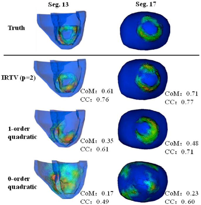
Two examples where the region of infarcts are located at anterior (Seg. 13) and apical (Seg. 17) regions of the LV, respectively.
Fig. 4.

Accuracy of (a) consistency metric and (b) correlation coefficient on 137 cases of infarcts with statistical analysis. Error bar shows the standard deviation of results.
Table I lists the COM and CC of all results with respect to the location and size of the infarct. wilcoxon rank tests and one-way ANOVA tests are used to compare how the results from IRTV differ, respectively, between all size groups and all location groups, except that of apical infarct due to the small sample size. As shown, it is more difficult to correctly capture the gradient of action potentials using IRTV when the infarct is located at the septal region of the LV (CoM: 0.34 ± 0.09; CC: 0.45 ± 0.16) compared to the anterior region (CoM: 0.52 ± 0.1, p < 0.01; CC: 0.62 ± 0.18, p < 0.01), or inferior region (CoM: 0.49 ± 0.07, p < 0.01; CC: 0.71 ± 0.09, p < 0.01), or lateral region (CoM: 0.54 ± 0.11, p < 0.01; CC: 0.73 ± 0.10, p < 0.01) of the LV (“±” interval represents the standard deviation). This is to be expected, because the septum is most hidden from body-surface observations and is consistent with some of our earlier observation in foci localization [39]. In comparison, there is no significant difference in the accuracy of IRTV (ANOVA p = 0.19) in outlining the gradient along infarcts of different sizes.
TABLE I.
Mean and Standard Deviation of Consistency Metric (CoM) and Correlation Coefficient (CC) Between the Reconstructed and True Regions of Steep Action Potential Gradients,With Respect to Infarct Locations (Top) and Sizes (Bottom)
| Segment | Anterior (n=26) | Inferior (n=21) | Lateral (n=40) | Septal (n=29) | Apex (n=4) | |||||
|---|---|---|---|---|---|---|---|---|---|---|
| CoM | CC | CoM | CC | CoM | CC | CoM | CC | CoM | CC | |
| IRTV(p =2) | 0.52 ± 0.10 | 0.62 ± 0.18 | 0.49 ± 0.07 | 0.71 ± 0.09 | 0.54 ± 0.11 | 0.73 ± 0.10 | 0.34 ± 0.09 | 0.45 ± 0.16 | 0.61 ± 0.13 | 0.67 ± 0.23 |
| 1-order | 0.36 ± 0.07 | 0.56 ± 0.17 | 0.32 ± 0.07 | 0.59 ± 0.13 | 0.40 ± 0.10 | 0.66 ± 0.11 | 0.27 ± 0.12 | 0.40 ± 0.17 | 0.47 ± 0.17 | 0.62 ± 0.29 |
| 0-order | 0.24 ± 0.06 | 0.37 ± 0.13 | 0.24 ± 0.05 | 0.39 ± 0.10 | 0.29 ± 0.08 | 0.38 ± 0.15 | 0.23 ± 0.07 | 0.32 ± 0.16 | 0.18 ± 0.09 | 0.28 ± 0.27 |
| Size | 0 ~ 5% (n=29) | 5% ~ 10% (n=31) | 10% ~ 20% (n=49) | ≥ 20% (n=28) | Total (n=137) | |||||
| CoM | CC | CoM | CC | CoM | CC | CoM | CC | CoM | CC | |
| IRTV (p=2) | 0.51 ± 0.10 | 0.64 ± 0.11 | 0.47 ± 0.14 | 0.61 ± 0.17 | 0.48 ± 0.13 | 0.65 ± 0.17 | 0.43 ± 0.11 | 0.65 ± 0.20 | 0.47 ± 0.13 | 0.64 ± 0.18 |
| 1-order | 0.33 ± 0.12 | 0.51 ± 0.15 | 0.34 ± 0.11 | 0.54 ± 0.16 | 0.35 ± 0.11 | 0.61 ± 0.16 | 0.35 ± 0.09 | 0.63 ± 0.20 | 0.34 ± 0.11 | 0.57 ± 0.17 |
| 0-order | 0.22 ± 0.07 | 0.34 ± 0.10 | 0.27 ± 0.09 | 0.41 ± 0.15 | 0.26 ± 0.07 | 0.34 ± 0.17 | 0.26 ± 0.04 | 0.34 ± 0.15 | 0.26 ± 0.07 | 0.36 ± 0.15 |
2). Variational TV-Prior Versus Discrete TV-Prior:
The chief motivation for the variational TV-prior, compared with L1-norm of discrete gradient field, is to 1) maintain robustness to different resolutions of the cardiac mesh, 2) reduce the computation cost of the regularization algorithm, and 3) simplify the calculation on an irregular mesh of heart. Here, we conduct a set of 72 studies to compare the performance of IRTV-L2 using the proposed variational definition in (13) versus traditional discrete definition of TV in (15). More specifically, the discrete gradient operator in discrete TV-form using (15) is constructed from the meshfree method. During the IR algorithm, the difference between these two TV definitions is exhibited as the way the re-weighting matrix is calculated in each iteration: WTW as defined in (14) for variational TV, versus DTWdD in (15) for discrete TV.
Fig. 5(a) and (b) shows the accuracy (consistency metric and correlation coefficient) of discrete TV and variational TV in preserving the steep gradient under different mesh resolutions (3–6 mm). As shown, variational TV delivers a more consistent accuracy among different resolutions than discrete TV, demonstrating a higher robustness to mesh resolutions as hypothesized. Similar observation is made in a recent study on quadratic regularization [40], where the optimal regularization parameter to balance between the data residual error and the regularization term is observed to vary less substantially when the regularization term is defined in a variational rather than discrete prior. Because the regularization parameter λ is automatically updated in our algorithm (see Algorithm 1), this type of phenomenon is not observed in our study.
Fig. 5.

Comparison study between discrete TV and variational TV: (a) CoM between the reconstructed and true regions of steep gradient; (b) CC between the reconstructed and true action potential; and (c) the time consumption of each iteration under the same operation system. Error bars in (a) and (b) show the standard deviation of results. (a) Consistency metric, (b) Correlation coefficient, (c) Time cost (s).
Fig. 5(c) shows the averaged computation cost per iteration for minimizing (6) using variational TV-prior and discrete TV-prior under different mesh resolutions (total number of iterations on average are similar). The computation time is reported using MATLAB with 2.66-GHz Intel Core 2 Duo. As the mesh resolution n increases, the discrete TV shows a substantially increasing demand in computation time as the dimension of the directional gradient operator D in (15) increases (3n × 3n). In comparison, the computation cost of variational TV remains stable, marginally affected by the mesh resolution and substantially lower than that of discrete TV for a dense mesh.
3). IRTV-L2 Versus IRTV-L1:
The comparison study between IRTV-L2 and IRTV-L1 is conducted with different levels of white Gaussian noises (6 dB, 10 dB, 15 dB, 20 dB, 25 dB, and 30 dB) added to the simulated 370-lead body-surface ECG as the input to reconstruct the 3-D action potential. We test 15 cases of infarct for each noise level and a total of 90 cases for each method.
Fig. 6(a) and (b) shows the accuracy of IRTV-L1 and IRTV-L2 in preserving the steep gradient of reconstructed action potential under different noise levels. As shown, IRTV-L1 is more robust to large measurement noises, while IRTV-L2 experiences a much faster deterioration of accuracy as the measurement noise increases. This result is consistent with other studies that compared L1-regularization with L2- versus L1-based data-fidelity term [15], [16], as would be expected because of the fundamental assumption behind a L1 data-fidelity term to handle measurement errors that are mostly small but occasionally large in space. For similar reasons, we expect that IRTV-L2 would deliver higher accuracy in the presence of low to moderate noises, as shown in our experimental results [Fig. 6(a) and (b)]. As an example, Fig. 7 compares the results of IRTV-L2 and IRTV-L1 in reconstructing the spatial distribution of action potential (a) and preserving its steep spatial gradient (b) along the border of an infarct located at anterior LV (segment 7, size 6.8%). With 25 dB measurement noise, the spatial structure of the steep gradient is well preserved by both IRTV-L2 and IRTV-L1, although IRTV-L2 shows a higher consistency with the ground truth (a sharper transition from necrotic to healthy tissue). When noise level is increased (e.g., 10 dB), the performance of IRTV-L2 drastically decreased while IRTV-L1 is still able to preserve the structure of the infarct border with reasonable accuracy.
Fig. 6.

Comparison of IRTV-L1 and IRTV-L2 methods at different noise levels: (a) consistency metric between the reconstructed and true regions of steep gradient; (b) correlation coefficient between the reconstructed and true action potential; and (c) number of iterations. The error bars in (a) and (b) show the standard deviation of results. (a) Consistency metric. (b) Correlation coefficient. (c) Average iterations.
Fig. 7.

Examples of IRTV-L1 and IRTV-L2 reconstruction of (a) action potential; and (b) steep action-potential gradient along infarct border at 25 dB noise and 10 dB noise. Color bars indicate the value of action potential and min-max gradient change, respectively.
Fig. 6(c) shows the averaged convergence speed (in terms of the number of iterations taken to convergence) of the two methods at different noise levels. As shown, IRTV-L1 takes a similar number of iterations to converge in the presence of different measurement noises, while IRTV-L2 takes much longer to converge as the noise level increases. As a result, with moderate-to-high level of measurement noise, IRTV-L1 shows faster convergence than IRTV-L2. Nevertheless, under the same computing environment, IRTV-L1 engages slightly more computation time (12.07 s) per iteration compared to IRTV-L2 (11.03 s). This is because, as shown in Algorithm 1 and Section III-C, IRTV-L1 involves two weight matrices in computation while IRTV-L2 has only one.
Given knowledge of measurement conditions, this set of experiments provides useful guidance on whether to use IRTV-L2 or IRTV-L1, given knowledge of measurement conditions. In the presence of low to moderate measurement noise, IRTV-L2 is preferred because of its higher accuracy and similar computation in comparison to IRTV-L1. In the presence of noisy measurements with high noise, IRTV-L1 should be used because of its robustness to measurement noise in both accuracy and computation time. In the rest of the phantom experiments (Section IV-C), we present results of IRTV-L2 with variational TV definition in comparison to quadratic regularization based methods.
B. Reconstruction Along Ischemic Regions
Myocardial ischemia is characterized by reduced blood supply to the heart muscle [41]. It is a precursor to myocardial infarction studied in Section IV-A. Physiologically, during induced ischemia such as the exercise test commonly used in clinical practice [42], the spatial pattern of action potential is similar to that of myocardial infarction: during the ST-segment of an ECG cycle, a localized gradient of action potential would be expected along the ischemic region. However, the magnitude of the gradient of action potential is expected to be smaller than that along an infarcted region as: [19], [43]
| (22) |
and
| (23) |
where t1 and t2 are, respectively, time instants during the plateau and resting state of the transmembrane action potential.
We carry out a set of initial studies to test the potential of IRTV in revealing the location of ischemic regions in the heart despite the lower value of gradient compared to that of an infarct. The location and extent of ischemic region are set in a similar manner to those of infarct as described above. The distribution of action potential values around the ischemic region is based on (22) and (23). In total, we test 30 cases of ischemic regions of different locations and sizes.
Across all 30 cases, the consistency metric obtained by IRTV-L2 versus the ground truth is 0.5416 ± 0.10 and the correlation coefficient is 0.71 ± 0.09. It shows no significant difference (p > 0.1) from the accuracy previously obtained in infarct experiments [Fig. 8(c)]. As an example, Fig. 8(a) and (b) compares the volumetric action potential estimated by IRTV-L2 with the ground truth, where the location of true ischemia region at lateral-basal LV (segment 5, size 4.1) is faithfully captured by IRTV-L2 both in the reconstructed action potential and its spatial gradient along the ischemic region.
Fig. 8.

Ischemia study results. Example of the action potential reconstruction of ischemia region in lateral region of heart: (a) ground truth setting; (b) IRTV-L2 the result from proposed method; and (c) the accuracy of reconstruction of 30 ischemic regions and statistical analysis.
This set of initial experiments shows the potential of IRTV-L2 to noninvasively detect the existence, location, and shape of ischemic region using only body-surface ECG data. With further investigations, IRTV-L2 has the potential to contribute to the unresolved issues of ischemia detection and diagnosis such as the low sensitivity and inability to locate ischemic lesions using the traditional 12-lead exercise testing [19].
C. Activation/Repolarization Wavefronts
We continue to extend IRTV to the reconstruction of action potential and its spatial gradient (localized excitation wavefront) during myocardial depolarization and repolarization, with a particular focus on its ability to capture disruption to electrical excitation wavefronts due to underlying conduction obstacles such as infarcted myocardial tissue. In this set of experiments, transmural propagation of ventricular action potential is simulated on 1230 meshfree nodes with the two-variable Aliev-Panfilov model [5] that has been widely used for forward simulations [5] as follows:
| (24) |
where v stands for recovery current and the matrix T is diffusion tensor and relies on the 3-D myocardial structure and its conductive anisotropy. T is considered anisotropic in this study, and its parameter values are adopted from [44]. Parameters e, k, and a determine individual action potential shape, where a represents tissue excitability of the myocardium. Here parameter a is set to be 0.5 for infarcts and 0.15 for healthy tissue [5]. Time sequences of 370-lead ECGs are simulated and corrupted with 20 dB white Gaussian noise. Selected time frames during activation or repolarization are used for IRTV reconstructions.
Depolarization:
Fig. 9 shows a sequence of snapshots of transmural action potential depolarization in a normal heart when the excitation propagates from the RV to LV and in comparison to the snapshots at the same time intervals on the same ventricles but with an infarct localized at the midbasal anterior region of the LV (labeled by purple line, size 8.5%). It is evident that the infarct works as a structural obstacle and reroutes the excitation of spatial action potential. The proposed IRTV-L2 captures the excitation wavefront in both normal and disrupted excitation, successfully revealing the underlying infarct that alters the excitation sequence. In comparison, the zeroth-order quadratic regularization fails to distinguish the depolarized region from the resting region in both cases. The first-order quadratic regularization partially captures the wavefront but not correctly on the endocardium; in particular, the excitation wavefront (spatial gradient of reconstructed action potential) appears to be much more diffused compared to IRTV results and the ground truth, and it fails to accurately capture the disruption to the wavefront caused by the infarct.
Fig. 9.

Examples of action potential mapping to show the change of propagation wavefronts in normal heart and infarct heart during depolarization. Left to right: 15, 22.5, 27.5, and 32.5 ms after the onset of ventricular activation. Border of an infarct region is outlined in purple.
Repolarization:
Fig. 10 shows a sequence of repolarization snapshots of the same normal and infarcted hearts where the infarct both disrupts the repolarization sequence and changes the action potential distribution along the infarct border in a way similar to that examined in previous sections. Again, the IRTV method is able to capture both the normal and disrupted action potential distribution, especially its spatial gradient that reveals the characteristics of the underlying infarct. In comparison, the other two quadratic-regularization methods fail to reveal the abnormal repolarization sequence related to the location or structure of the infarct.
Fig. 10.

Change of propagation wavefronts in normal heart and infarct heart during repolarization. Left to right: 80, 85, 95, and 105 ms after the onset of ventricular activation. Border of an infarct region is outlined in purple.
Fig. 11 shows another example of action potential sequence in healthy versus infarcted hearts where similar results can be observed. Both the spatial distribution of action potential and its spatial gradient (wavefront) are displayed to better illustrate the ability of IRTV to faithfully capture the change of transmural electrical excitation while the quadratic-regularization methods fail to do so.
Fig. 11.

Change of excitation wavefronts in normal and infarcted hearts. Depolarization stage shows the steep gradient of action potential. Repolarization stage is illustrated by action potential (AP) map and the corresponding gradient of action potential (gradient). Purple arrow shows the propagation direction and purple contour indicates the border of an infarct region.
V. Human Study
Real-data experiments are performed on two post-infarction patients with MRI and body-surface ECG data made available to this study by the 2007 PhysioNet/Computers in Cardiology Challenges [45]. Short-axis (SA) cardiac MRI of each patient contains ten slices from apex to base of the ventricles, with 8-mm inter-slice spacing and 1.33 mm/pixel in-plane resolution.
Body-surface ECG were recorded by the Dalhousie University protocol [46], [47] at 120 pre-specified torso positions plus three limb leads; each body-surface ECG recording [Fig. 12(a)] consists of a single QRST complex averaged from 15 s recordings sampled at 2 kHz. For each patient, a late gadolinium-enhanced (LGE) MRI was obtained for delineating the region of infarct. Because measurement data on cardiac electrical excitation is not available, here we focus on the performance of IRTV in reconstructing the action potential and its spatial gradient along the infarct border during the ST-segment of an ECG cycle.
Fig. 12.

Input ECG traces and the snapshot of body-surface-potential map at the time instant selected for experiment input in case 1 (labeled by the red line on the ECG trace). (a) An ECG cycle. (b) Body surface ECG at 573 ms.
Ventricular models for both patients were built from their MRI as described in [30]. A homogenous torso model of each patient was obtained by deforming the standard Dalhousie torso model given by the 2007 PhysioNet/Computers in Cardiology Challenges to limited whole-body MR scans of each patient via host mesh customization method [5]. From each patient’s body-surface mapping data, we select a time frame within the ST interval (for ventricular electrical activity) as input. Fig. 12 illustrates an ECG cycle and the selected input body-surface potential map at 573 ms for case 1. Gold standards of infarct quantification were obtained from LGE MRI by cardiologists blinded to this study. Unlike phantom experiments, the gold standards and existing results quantify the location and size of the infarct according to the standard AHA 17-segment model of LV, revealing core regions of the infarct as labelled by the red cycle in Figs. 13 and 14 and Table II. In order to compare with the gold standard, we also quantify the infarct region according to AHA 17-segment using segment overlap (SO) that measures the percentage of correctly identified segments [5], , where Segr refers to the segments of reconstruction and Segt refers to the segments defined in ground truth.
Fig. 13.
Results of case 1. Spatial gradients of transmural action potential reconstructed from IRTV-L2, IRTV-L1, and quadratic methods on one post-infarction human heart. Red cycle represents the core of the MRI-delineated infarcts. (a) IRTV-L2. (b) IRTV-L1. (c) First-order. (d) Zeroth-order.
Fig. 14.

Results of case 2. Spatial gradients of transmural action potential reconstructed from IRTV-L2, IRTV-L1, and quadratic methods on another post-infarction human heart. Red cycles represent the core of the MRI-delineated infarcts. (a) IRTV-L2. (b) IRTV-L1. (c) Zeroth-order.
TABLE II.
Infarct Quantification Results From IRTV-L2 Compared With Provided Gold Standard Which Quantifies the Location of Infarct According to the AHA 17-Segment Model of LV
| Center (CE) | Location | Segment overlap (SO) | ||
|---|---|---|---|---|
| Case 1 | Gold standard | 10/11 | 3,4,5,9,10,11,12,15,16 | NA |
| IRTV-L2 | 10/15 | 3,8,9,10,11,12,14,15,17 | 66.7% | |
| Case 2 | Gold standard | 15 | 1,9,10,11,15,17 | NA |
| IRTV-L2 | 15 | 1,7,9,10,11,15,17 | 75.0% |
The patient of case 1 has a single infarct with its core located at middle septal-inferior LV (segment 9 and segment 10). As shown in Fig. 13, spatial distribution of action potential reconstructed by IRTV-L2 exhibits a steep gradient that is localized and distributed along the MRI-delineated infarct core. A similar result is found with IRTV-L1. In comparison, the action potentials reconstructed from either of the other two quadratic methods do not provide any physiologically meaningful information regarding the existence, location, or structure of the infarct.
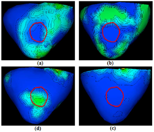
The patient of case 2 has two separated regions of infarct (Fig. 14), one at basal–anterior LV (segment 1) and the other at apical–inferior LV (segment 15). Previous attempts to resolve these two separate infarct regions have failed [5], [48]–[50]. As shown in Fig. 14, spatial gradients of action potential reconstructed by IRTV-L2 are correctly localized around both infarcts, revealing the location and extent of both infarct cores. IRTV-L1, in comparison, partially misses the localization of one infarcted region. Perhaps this is because that the 120-lead data did not have high measurement noise and thus the assumption behind IRTV-L1 does not hold as shown in Section IV-A3. The zeroth-order quadratic method only reveals certain information in the inferior ventricular wall (right) without revealing any physiologically meaningful structure along the infarct, and it loses all the information in the anterior wall (left). First-order quadratic method fails to detect the infarct regions under all possible parameters using the cvx software mentioned in [18], [51]. These observations in real-data study are consistent with the findings in our phantom experiments.
Table II lists quantification comparison with the gold standard. As shown, the ischemic centers are correctly identified in both patients and the accuracy is comparable to the best result available [5], [49], [50]. In particular, in case 2 our method shows much higher accuracy in localizing the two separated ischemic regions with segment overlap SO = 75.0%, while the best available SO reported in the literature was 33.33.
VI. Discussion
A. Initialization
The use of sparsity-based TV-minimization in the proposed method of IRTV focuses on overcoming the physical ill-posedness of this problem. Therefore, a proper initialization is needed to first overcome the mathematical ill-possedness, based on the best available low-resolution estimate of the sparse solution. In the current study, we use a simple zeroth-order Tikhonov regularization as initialization for IRTV. Our experiments show that smoothness-enforcing regularization methods (such as different orders of Tikhonov regularization) are in general suitable choices for IRTV initialization. For example, Fig. 15 shows a randomly selected data set of 28 quantitative analysis of IRTV results based on two different initialization methods: 0-order Tikhonov regularization versus weighted minimum norm [17]. The Wilcoxon rank test shows that the accuracies of IRTV have no significant difference (p > 0.3) when initialized by these two different methods. From our experience and experimental studies, we conclude that the final results of IRTV will not be significantly affected as long as the initialization methods satisfy the following requirements: 1) the results should be “blurred” with the smoothness assumption that overcomes the mathematical ill-posedness; 2) all the entries in the results should be nonzero so that potentially important components are not lost before being pruned by the sparsity-enforcing IRTV.
Fig. 15.

Comparison of the accuracy of IRTV in preserving the steep gradient based on two different initialization methods (zeroth-order Tikhonov regularization and weighted minimum norm) for randomly selected data sets. Wilcoxon rank test shows there is no significantly difference between these two sets of results.
B. Parameter Selection
One of the critical factors in the proposed IRTV is the regularization parameter λ, an improper high or low value of which will lead to a neglect of either the data fidelity or the TV-prior during the optimization. unlike the quadratic regularization where it is established that the value of λ could be determined by methods such as L-curve, there is not yet any established method for objective and optimal selection of a regularization parameter for L1-norm regularization. Consequently, most existing methods rely on an empirical procedure through a substantial amount of supervision to select an suboptimal value of λ after a large set of experiments [35], [36]. This trial-and-error procedure is not suitable for the proposed iterative reweighted methods because the optimal regularization parameter λ(k) is expected to change at each iteration k due to the change of the weight in the prior weighted L2-norm. Therefore, we adopt a more robust and objective method that sets the magnitude of λ basedon the infinity norm of the data-fidelity and TV terms to roughly balance their relative importance in the regularization. This parameter selection method also can reduce the method’s sensitivity to the value of the regularization parameter λ, which makes IRTV more stable.
The other parameter β in (17) is a control parameter to avoid numerical difficulty as ∣∇φiu(k–1) approaches 0 in the denominator of (17). The common practice is to set a smaller value of 10−7 for β.
C. Infarction or Ischemia Setting
Physiologically, during the plateau and resting state, the value of transmembrane action potential in the healthy versus ischemic tissue can be expressed in (22), (23). This setting has been commonly used in existing simulation studies on the detection of ischemic or infarcted regions [19]. Here we tested the proposed IRTV in ischemic/infarction detection based on this physiological setting versus the simplified setting where the action potential value is normalized within 0–1 from the physiological range of a −80–20 mV. Fig. 16 shows the results of IRTV on these two settings from 25 randomly selected data sets. As shown, changing between these two experimental settings does not cause significant difference (p > 0.2) in the accuracy of the gradient of reconstructed action potential in terms of its consistency measure with ground truth. However, the simplified setting with a 0–1 instead of −80–20 range significantly reduces the computational time of IRTV (27 versus 89 iterations on average). Considering the slight influence on IRTV accuracy and the substantial difference of computation time between the two experimental settings, the large set of simulation studies in this paper is mostly conducted on the simplified setting without loss of physiological plausibility.
Fig. 16.
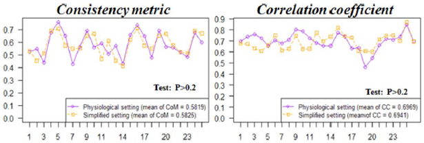
Comparison of the accuracy of IRTV in preserving the steep gradient based on two different experiment action potential setting (physiological setting and simplified 0–1 setting) for randomly selected data sets. Wilcoxon rank test shows there is no significant difference between two settings.
D. Effect of Geometrical Modeling Errors
In order to investigate the stability of the IRTV method, we perform a preliminary study to test how this method could be affected by small geometrical modeling errors reflected in H. We perturb the position and orientation of the heart model to add errors in the H matrix and use it for the inverse method. We test four different cases of infarcted hearts for each change, including two cases with the heart position moved into right direction with 1 mm distance and the other two cases with the heart orientation turned clockwise 5°. Fig. 17 shows the accuracy of the IRTV method under different modeling errors. As shown, the value of CoM and CC does not change significantly compared with the results where no geometrical errors are introduced. It seems that the IRTV method has potential to deal with moderate modeling errors. As the standard practice in the filed of EEG-based noninvasive EP imaging, H is considered time-invariant in our study to disregard cardiac deformation and motion. This assumption is expected to have little impact on electrical depolarization because of its short time span preceding the contraction of the heart muscle. However, it will affect the reconstruction during electrical repolarization phase, and future work will investigate the possibility to combine cardiac motion into noninvasive EP imaging. Additionally, in the current study we investigate the influence of the resolution of meshfree points on the proposed method. In the future, we will investigate the influences from not only the number but the distribution of meshfree points.
Fig. 17.

Comparison of the accuracy (CoM and CC) of proposed IRTV method in different geometrical modeling errors (position error and orientation error) for 4 test cases.
VII. Conclusion
This paper presents a novel approach to transmural electrophysiological imaging based on the introduction of spatial TV-prior. This approach is physiologically motivated by the unique spatial property of transmural action potential that is piecewise smooth with sharp boundaries in between. It is also closely tied to the boundary separating ischemic and nonischemic regions, which is one of the most important regions in the genesis of lethal arrhythmia. Through a large set of simulation studies as well as two initial clinical studies on post-infarction human subjects, we demonstrate the superiority of the proposed method over existing quadratic methods in revealing the location and shape of the underlying substrates for cardiac arrhythmia. In this study, IRTV is carried out at each separate time interval without considering any temporal constraints on the electrical excitation; our initial experiments (Section IV-C) show that it is able to reflect the temporal trace of electrical excitation in this manner. Nevertheless, temporal trace of action potential also contains rich physiological information that should be incorporated into the inverse problem. The next immediate step of our future work is to integrate the spatial TV-prior with temporal knowledge of action potential dynamics [52] to improve the accuracy and temporal consistency of the proposed method.
Acknowledgments
This work is supported by the National Science Foundation CAREER-Award ACI-1350374.
Contributor Information
Jingjia Xu, Computational Biomedicine Laboratory, Golisano College of Computing and Information Sciences, Rochester Institute of Technology, Rochester, NY 14623 USA (jxx2144@rit.edu)..
Azar Rahimi Dehaghani, Computational Biomedicine Laboratory, Golisano College of Computing and Information Sciences, Rochester Institute of Technology, Rochester, NY 14623 USA..
Fei Gao, Molecular Imaging Division, Siemens Medical Solutions, Knoxville, TN 37932 USA..
Linwei Wang, Computational Biomedicine Laboratory, Golisano College of Computing and Information Sciences, Rochester Institute of Technology, Rochester, NY 14623 USA..
References
- [1].Fuster V and Kelly EBB, Promoting Cardiovascular Health in the Developing World: A Critical Challenge to Achieve Global Health.. Washington DC: Nat. Acad. Press, 2010. [PubMed] [Google Scholar]
- [2].Frangi AF, Niessen WJ, and Viergever MA, ”Three-dimensional modeling for functional analysis of cardiac images, a review,” IEEE Trans. Med. Imag, vol. 20, no. 1, pp. 2–5, January 2001. [DOI] [PubMed] [Google Scholar]
- [3].Wong KC, Zhang H, Liu H, and Shi P, “Physiome-model-based state-space framework for cardiac deformation recovery, ” Acad. Radiol, vol. 14, no. 11, pp. 1341–1349, 2007. [DOI] [PubMed] [Google Scholar]
- [4].Sermesant M, Moireau P, Camara O, Sainte-Marie J, Andriantsimiavona R, Cimrman R, Hill DL, Chapelle D, and Razavi R, “Cardiac function estimation from MRI using a heart model and data assimilation: Advances and difficulties,” Med. Imag. Anal, vol. 10, no. 4, pp. 642–656, 2006. [DOI] [PubMed] [Google Scholar]
- [5].Wang L, Wong KC, Zhang H, Liu H, and Shi P, “Noninvasive computational imaging of cardiac electrophysiology for 3-D infarct,” IEEE Trans. Biomed. Eng, vol. 58, no. 4, pp. 1033–1043, April 2011. [DOI] [PubMed] [Google Scholar]
- [6].Plonsey R, Bioelectric Phenomena. New York: Wiley Online Library, 1999. [Google Scholar]
- [7].Rudy Y and Messinger-Rapport B, “The inverse problem in electrocardiography: Solutions in terms of epicardial potentials,” Crit. Rev. Biomed. Eng, vol.16, no.3, p.215, 1988. [PubMed] [Google Scholar]
- [8].Ramanathan C, Ghanem RN, Jia P, Ryu K, and Rudy Y, “Noninvasive electrocardiographic imaging for cardiac electrophysiology and arrhythmia,” Nat. Med, vol. 10, no. 4, pp. 422–28, 2004. [DOI] [PMC free article] [PubMed] [Google Scholar]
- [9].van Dam P, Oostendorp T, Linnenbank A, and van Oosterom A, “Noninvasive imaging of cardiac activation and recovery,” Ann. Biomed. Eng, vol. 37, no. 9, pp. 1739–1756, 2009. [DOI] [PMC free article] [PubMed] [Google Scholar]
- [10].Serinagaoglu Y, Brooks DH, and MacLeod RS, “Improved performance of Bayesian solutions for inverse electrocardiography using multiple information sources,” IEEE Trans. Biomed. Eng, vol. 53, no. 10, pp. 2024–2034, October 2006. [DOI] [PubMed] [Google Scholar]
- [11].Rudy Y and Oster H, “The electrocardiographic inverse problem,” Crit. Rev. Biomed. Eng, vol. 20, no. 1–2, p. 25, 1992. [PubMed] [Google Scholar]
- [12].Okamoto Y, Teramachi Y, and Musha T, “Limitation of the inverse problem in body surface potential mapping,” IEEE Trans. Biomed. Eng, no. 11, pp. 749–754, November 1983. [DOI] [PubMed] [Google Scholar]
- [13].Messnarz B, Tilg B, Modre R, Fischer G, and Hanser F, “A new spatiotemporal regularization approach for reconstruction of cardiac transmembrane potential patterns,” IEEE Trans. Biomed. Eng, vol. 51, no. 2, pp. 273–281, February 2004. [DOI] [PubMed] [Google Scholar]
- [14].Brooks DH, Ahmad GF, MacLeod RS, and Maratos GM, “Inverse electrocardiography by simultaneous imposition of multiple constraints,” IEEE Trans. Biomed. Eng, vol. 46, no. 1, pp. 3–18, January 1999. [DOI] [PubMed] [Google Scholar]
- [15].Ghosh S and Rudy Y, “Application of L1-norm regularization to epicardial potential solutions of the inverse electrocardiography problem,” Ann. Biomed. Eng, vol. 37, no. 5, pp. 902–912, 2009. [DOI] [PMC free article] [PubMed] [Google Scholar]
- [16].Shou G, Xia L, and Jiang M, “Total variation regularization in electrocardiographic mapping,” in Life System Modeling and Intelligent Computing. New York: Springer, 2010, vol. 6330, pp. 51–59. [Google Scholar]
- [17].He B and Wu D, “Imaging and visualization of 3-D cardiac electric activity,” IEEE Trans. Inf. Tech. Biomed, vol. 5, no. 3, pp. 181–186, September 2001. [DOI] [PubMed] [Google Scholar]
- [18].Wang D, Kirby RM, MacLeod RS, and Johnson CR, “Identifying myocardial ischemia by inversely computing transmembrane potentials from body-surface potential maps,” in Int. Conf. Bioelectromagn, Salt Lake, UT, 2011, pp. 121–125. [Google Scholar]
- [19].Nielsen BF, Lysaker M, and Grøttum P, “Computing ischemic regions in the heart with the bidomain model: First steps towards validation,” IEEE Trans. Med. Imag, vol. 32, no. 6, pp. 1085–1096, June 2013. [DOI] [PubMed] [Google Scholar]
- [20].He B, Li G, and Zhang X, “Noninvasive imaging of cardiac transmembrane potentials within three-dimensional myocardium by means of a realistic geometry anisotropic heart model,” IEEE Trans. Biomed. Eng, vol. 50, no. 10, pp. 1190–1202, October 2003. [DOI] [PubMed] [Google Scholar]
- [21].Chambolle A, “An algorithm for total variation minimization and applications,” J. Math. Imag. Vis, vol. 20, no. 1–2, pp. 89–97, 2004. [Google Scholar]
- [22].Rudin LI, Osher S, and Fatemi E, “Nonlinear total variation based noise removal algorithms,” Phys. D: Nonlinear Phenom, vol. 60, no. 1, pp. 259–268, 1992. [Google Scholar]
- [23].Chan T and Wong CK, “Total variation blind deconvolution,” IEEE Trans. Image Process, vol. 7, no. 3, pp. 370–375, March 1998. [DOI] [PubMed] [Google Scholar]
- [24].Chan T, Shen J, and Zhou H, “Total variation wavelet inpainting,” J. Math. Imag. Vis, vol. 25, no. 1, pp. 107–125, 2006. [Google Scholar]
- [25].Rodríguez P and Wohlberg B, “Efficient minimization method for a generalized total variation functional,” IEEE Trans. Image Process, vol. 18, no. 2, pp. 322–332, February 2009. [DOI] [PubMed] [Google Scholar]
- [26].Liu Z, Liu C, and He B, “Noninvasive reconstruction of three-dimensional ventricular activation sequence from the inverse solution of distributed equivalent current density,” IEEE Trans. Med. Imag, vol. 25, no. 10, pp. 1307–1318, October 2006. [DOI] [PubMed] [Google Scholar]
- [27].Schmidt A, Azevedo CF, Cheng A, Gupta SN, Bluemke DA, Foo TK, Gerstenblith G, Weiss RG, Marbán E, and Tomaselli GF, “Infarct tissue heterogeneity by magnetic resonance imaging identifies enhanced cardiac arrhythmia susceptibility in patients with left ventricular dysfunction,” Circulation, vol. 115, no. 15, pp. 2006–2014, 2007. [DOI] [PMC free article] [PubMed] [Google Scholar]
- [28].Hren R, Nenonen J, and Horáček BM, “Simulated epicardial potential maps during paced activation reflect myocardial fibrous structure,” Ann. Biomed. Eng, vol. 26, no. 6, pp. 1022–1035, 1998. [DOI] [PubMed] [Google Scholar]
- [29].Wang L, Zhang H, Wong KC, and Shi P, “Coupled meshfree-BEM platform for electrocardiographic simulation: Modeling and validations,” in Medical Imaging and Augmented Reality. New York: Springer, 2008, pp. 98–107. [Google Scholar]
- [30].Wang L, Zhang H, Wong KC, and Liu H, “Electrocardiographic simulation on personalised heart-torso structures using coupled meshfree-BEM platform,” Int. J. Funct. Inform. Personal. Med, vol. 2, no.2 pp. 175–200, 2009. [Google Scholar]
- [31].Fischer G, Tilg B, Modre R, Huiskamp G, Fetzer J, Rucker W, and Wach P, “A bidomain model based BEM-FEM coupling formulation for anisotropic cardiac tissue,”Ann. Biomed. Eng, vol. 28, no. 10, pp. 1229–1243, 2000. [DOI] [PubMed] [Google Scholar]
- [32].Li Y and Santosa F, “A computational algorithm for minimizing total variation in image restoration,” IEEE Trans. Image Process, vol. 5, no. 6, pp. 987–995, June 1996. [DOI] [PubMed] [Google Scholar]
- [33].Belytschko T, Krongauz Y, Organ D, Fleming M, and Krysl P, “Meshless methods: An overview and recent developments,” Comput. Methods Appl. Mech. Eng, vol. 139, no. 1, pp. 3–47, 1996. [Google Scholar]
- [34].Hansen P and O’Leary D, “The use of the L-curve in the regularization of discrete ill-posed problems,” SIAMJ. Sci. Comput, vol. 14, no. 6, pp. 1487–1503, 1993. [Google Scholar]
- [35].Candès EJ and Plan Y, “Near-ideal model selection by L1 minimization,” Ann. Stat, vol. 37, no. 5A, pp. 2145–2177, 2009. [Google Scholar]
- [36].Ou W, Hämäläinen MS, and Golland P, “A distributed spatio-temporal EEG/MEG inverse solver,” NeuroImage, vol. 44, no. 3, pp. 932–946, 2009. [DOI] [PMC free article] [PubMed] [Google Scholar]
- [37].Schmidt M, Fung G, and Rosales R, Optimization methods for L1-regularization Univ. British Columbia, Tech. Rep. TR-2009-19, 2009. [Google Scholar]
- [38].Cerqueira MD, Weissman NJ, Dilsizian V, Jacobs AK, Kaul S, Laskey WK, Pennell DJ, Rumberger JA, Ryan T, and Verani MS, “Standardized myocardial segmentation and nomenclature for tomographic imaging of the heart a statement for healthcare professionals from the Cardiac Imaging Committee of the Council on Clinical Cardiology of the American Heart Association,” Circulation, vol. 105, no. 4 pp. 539–542, 2002. [DOI] [PubMed] [Google Scholar]
- [39].Xu J, Dehaghani AR, Gao F, and Wang L, “Localization of sparse transmural excitation stimuli from surface mapping,” in Med. Image. Comput. Comput. Assist. Interv. (MICCAI). New York: Springer, 2012, pp. 675–682. [DOI] [PubMed] [Google Scholar]
- [40].Wang D, Kirby RM, and Johnson CR, “Finite-element-based discretization and regularization strategies for 3-D inverse electrocardiography,” IEEE Trans. Biomed. Eng, vol. 58, no. 6, pp. 1827–1838, June 2011. [DOI] [PMC free article] [PubMed] [Google Scholar]
- [41].Jennings R, Steenbergen C Jr., and Reimer K, “Myocardial ischemia and reperfusion,” Monogr. Pathol, vol. 37, pp. 47–80, 1994. [PubMed] [Google Scholar]
- [42].James DYS and Hansen E, Principles of Exercise Testing and Interpretation: Including Pathophysiology and Clinical Applications, Wasserman KSK, Ed. New York: Wolters Kluwer Health/Lippincott Williams & Wilkins, 2011. [Google Scholar]
- [43].Barrett TD, MacLeod BA, and Walker MJ, “A model of myocardial ischemia for the simultaneous assessment of electrophysiological changes and arrhythmias in intact rabbits,” J. Pharmacol. Toxicol. Methods, vol. 37, no. 1, pp. 27–36, 1997. [DOI] [PubMed] [Google Scholar]
- [44].Aliev RR and Panfilov AV, “A simple two-variable model of cardiac excitation,” Chaos, Solitons Fractals, vol. 7, no. 3, pp. 293–301, 1996. [Google Scholar]
- [45].Goldberger AL, Amaral LA, Glass L, Hausdorff JM, Ivanov PC, Mark RG, Mietus JE, Moody GB, Peng C-K, and Stanley HE, “Physiobank, physiotoolkit, and physionet: Components of a new research resource for complex physiologic signals,” Circulation, vol. 101, no. 23, pp. e215–e220, 2000. [DOI] [PubMed] [Google Scholar]
- [46].Warren JW, Penney CJ, MacLeod RS, Gardner MJ, and Feldman CL, “Optimal electrocardiographic leads for detecting acute myocardial ischemia,” J. Electrocardiol, vol. 34, no. 4, pp. 97–111, 2001. [DOI] [PubMed] [Google Scholar]
- [47].Title LM, Iles SE, Gardner MJ, Penney CJ, Clements JC, and Horáček BM, “Quantitative assessment of myocardial ischemia by electrocardiographic and scintigraphic imaging,” J. Electrocardiol, vol. 36, pp. 17–26, 2003. [DOI] [PubMed] [Google Scholar]
- [48].Dawoud F, Wagner GS, Moody G, and Horáček BM, “Using inverse electrocardiography to image myocardial infarction-reflecting on the 2007 physionet/computers in cardiology challenge,” J. Electrocardiol, vol. 41, no. 6, pp. 630–635, 2008. [DOI] [PubMed] [Google Scholar]
- [49].Farina D and Dossel O, “Model-based approach to the localization of infarction,” in IEEE Comput. Cardiol, September 2007, pp. 173–176. [Google Scholar]
- [50].Mneimneh M and Povinelli R, “RPS/GMM approach toward the localization of myocardial infarction,” in IEEE Comput. Cardiol, September 2007, pp. 185–188. [Google Scholar]
- [51].Grant M, Boyd S, and Ye Y, CVX: Matlab software for disciplined convex programming [Online]. Available: http://cvxr.com/tfocs/down-load/, 2008
- [52].Wang L, Dawoud F, Yeung S-K, Shi P, Wong K, and Lardo A, “Transmural imaging of ventricular action potentials and post-infarction scars in swine hearts,” IEEE Trans. Med. Imag, vol. 32, no. 4, pp. 731–747, April 2013. [DOI] [PubMed] [Google Scholar]