Variability of Betweenness Centrality and Its Effect on Identifying Essential Genes

Abstract

This paper begins to build a theoretical framework that would enable the pharmaceutical industry to use network complexity measures as a way to identify drug targets. The variability of a betweenness measure for a network node is examined through different methods of network perturbation. Our results indicate a robustness of betweenness centrality in the identification of target genes.

1. Introduction

Current technology provides the clinician with high-dimensional measurements that describe features of a particular tissue, or cellular environment. For example, we might have flow-cytometry data that quantify multiple markers in a given sample, or we might have gene expression data for samples of cells that can be divided into “healthy” and “diseased” groups. Figure 1 shows a heat map of gene expression data from thirty tissue samples, sixteen healthy samples and fourteen tumor samples.

Fig. 1.

A heat map showing gene expression data from 30 tissue samples. The 16 samples on the left are from healthy tissue; the 14 samples on the right are from tumor samples. Each horizontal row is one gene, and the columns are different samples. Colors show expression levels. In this study, we sought to define differences between neoplastic and non-neoplastic groups. Specifically, we were interested in answering this question in the context of changes in the network that represent the interactions between genes. In other words, how can we identify the genes that play important roles in these network changes? Data are from the publicly available NCBI GEO repository, GSE42656.

One question that we would like to answer using these data is: “What is the difference between the healthy and the diseased groups?” Standard t-tests are problematic in that they do not allow for the analysis to harness the global structure of the data, instead looking at each gene as a separate sample. Some differential expression analyses use pooled methods for estimating variability, but differential expression alone misses important structure between genes. One approach to addressing the comparative question of healthy versus diseased is motivated by advances in systems biology. The cell is first described as an interacting network of genes or proteins, and then the data are used to understand how the strengths of the connections in the given network change in comparing healthy and diseased tissues. The goal of many of these studies of biological networks is to identify “essential” or “hub” nodes in the network; see, for example, [1–3].

In this paper, we focus on the use of network centrality measures to identify nodes, i.e. genes that are highly associated with changes in the network. The use of an array of network centrality measures has been used in this context for a variety of applications [4–9]. In [10] we used betweenness, one such centrality measure, to identify ETV5 as a key regulator in the development of optic glioma. In this paper, we use the term essential in a precise way to identify genes that meet two threshold criteria based on a centrality measure.

Definition 1.

Let A and B be two networks with the same nodes and edges, but different edge weights, and let T1 and T2 be two threshold values. We define a node v to be essentially different if the ratio:

$$\frac{\mathit{betweenness\; of\; v\; in\; network\; A}}{\mathit{betweenness\; of\; v\; in\; network\; B}}>T_1,\mathit{and\; betweenness\; of\; node\; v}>T_2.$$

In [10], we found that ETV5 was essentially different when comparing a network from tumor samples to a network based on normal optic nerve samples. In that work, we were able to experimentally validate ETV5 as a central regulator. In general, however, we would like to have an analytic method to gauge the robustness of the betweenness centrality as a method for identifying key regulators. That desire is the motivation for the current work.

To put our work in context, we will consider the betweenness network centrality measure as a parameter describing a population network derived from the entire population of, for example, tumor patients of interest.

Definition 2.

A parameter is a numerical summary value of the population from which the data are obtained.

In our case, the topology, or structure of the network, is fixed: all of the networks work in the collection have the same number of nodes and the same edges connecting the nodes. The individual networks differ only in the weights assigned to each edge. We can characterize a particular weighted network in the collection by the centrality measures of its set of nodes. In other words, the centrality measure of each node is a parameter of this family of networks. Our theoretical assumption is that one weighted network represents “healthy” tissue, and one represents “diseased” tissue, for example tissue corresponding to a particular tumor. Thus, the value of the parameter representing the centrality of a particular node might allow us to distinguish between healthy tissue and a tumor. In our construction, the weights on the network edges are assigned by using correlations between expression levels of each gene represented as a node. The theoretical networks have edge-weights determined by the “true” correlations between the genes, i.e. the correlations are determined using all instances of “normal” or “tumor” tissue. In practice, the edge-weights are assigned using correlations between relatively few samples. Thus, we only get an estimate of the true centrality measure of each node; in mathematical terminology, we consider the estimated centrality a statistic that is our best estimate of the true parameter.

Definition 3.

A statistic is a numerical summary value of a sample from the population.

This interpretation suggests the following important question: how accurate is this estimate? How robust is the statistic to sampling variability? How meaningful is a specific difference between this same statistic obtained from two different groups of samples?

A variety of network centrality measures, some in combination with other biological information, has been used to identify genes that are important in the development of a disease; examples of such studies are [11–14]. The potential impact of this research, coupled with the questions that we ask in the preceding paragraph, point to a need for a theoretical framework to understand the variability of centrality measures as statistics of biological networks. Some work has been done in this direction. In [15], Segarra and Rubeiro provide formal definitions of stability and continuity for centrality measures in weighted networks. They show that betweenness centrality is neither stable nor continuous according to these definitions, and propose an alternative definition of betweenness that is stable. Epskamp et al. take a statistical approach, more similar to ours [16]. They discuss the stability of centrality rankings in terms of how these rankings might change with fewer observations. They also describe how to test whether differences in centrality measures between groups are significant by introducing a boot-strapped difference test for centrality indices. The methods are applied to a psychological network.

This paper adds to the theoretical framework by considering a collection of networks with fixed topology. We propose a methodology for producing confidence intervals for centrality statistics, and we illustrate the methodology by applying it to the network and data previously discussed in [10]. The methods can be generally applied to other situations where samples of high-dimensional data are used to identify targets for clinical intervention in the progression of a disease.

The paper is organized as follows. Relevant definitions are detailed in Section 2. The methodology to measure the variability of betweenness is presented in Section 3. In Section 4, the centrality variability procedures are applied to pediatric brain tumors relative to control brain tissue. Results and future work are discussed in Section 5.

2. Background

Nodes in biological networks can be characterized by a set of centrality measures. Therefore, as described above, these measures could be used to identify structural differences between biological networks representing two different states of a particular tissue. In this paper, we investigate how perturbations to the edge-weights given on a known network structure influence the variability of one centrality measure, betweenness. Although betweenness is, in general, not continuous, as defined in [15], we show that betweenness can be used to discriminate between networks based on healthy and tumor samples. Below we define terminology and concepts relevant to our analysis.

2.1. Network Definitions

Formally, we define a biological network as an abstract, undirected, and weighted graph G = (V; E) where V is the set of nodes representing biological molecules (i.e., genes and proteins), and E is the set of edges representing the functional, causal, or physical interactions between nodes that is associated with a weight function $w:E\to {ℝ}^n\ge 0.$ We denote the set of edges by $E=\left\{e_{i,j}|v_i,v_j\in V\right\}$ the set of connections between nodes v_i and v_j of strength $w\left(e_{i,j}\right)=w_{i,j}.$ Any two nodes connected by an edge are considered adjacent, and we define a path, P, as a sequence of edges that connect adjacent nodes:

$$P=\left\{e_{i_1,i_2},e_{i_2,i_3},\dots ,e_{i_k,i_{k+1}},\dots ,e_{i_{n-1},i_n}\right\}$$

where edge $e_{i_k,i_{k+1}}$ connects adjacent nodes $v_{i_k}$ and $v_{i_{k+1}}$ for $1\le k\le n.$ The length of a path P is the sum of the edge-weights of the edges in P. Finally, a shortest path between nodes v_i and v_j is a path of minimum length, which we will denote by P_s.

An example of a weighted network can be seen in Figure 2. While we may define a path from node 1 to node 4 as $P=\left\{e_{1,2},e_{2,3},e_{3,4}\right\},$ we see that a shortest path between these nodes as $P_s=\left\{e_{1,3},e_{3,4}\right\}$.

Fig. 2.

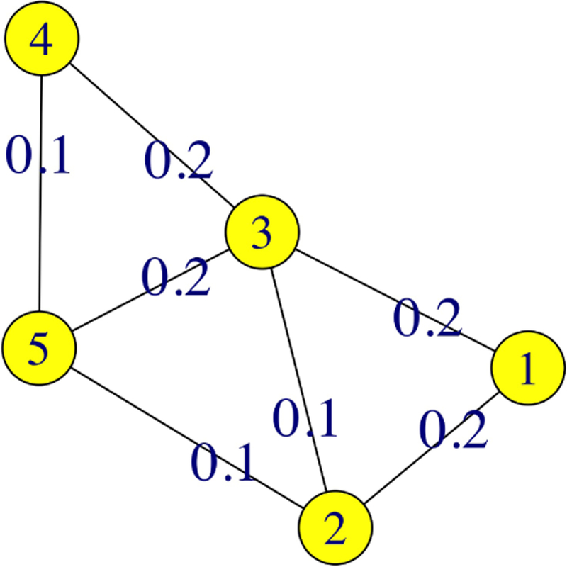
A weighted sample network with nodes V = {1, 2, 3, 4, 5} and edges E = {e_1,2, e_1,3, e_2,3, e_2,5, e_3,4, e_3,5, e_4,5} with corresponding edge-weights {0.2, 0.2, 0.1, 0.1, 0.2, 0.2, 0.1}.

2.2. Network Centrality Measures

Network nodes can be characterized by several centrality measures, all of which evaluate their importance through a partial ranking based upon the network’s topological features and edge-weights. Below we define the betweenness centrality measure, while a more complete treatment of centrality measures can be found elsewhere [17, 18].

2.2.1. Betweenness Centrality

Betweenness centrality quantifies the involvement of a node in the shortest paths of a network [5]. For every pair of nodes in a connected network, there exists at least one shortest path.

The betweenness centrality of node v_i in a network is computed as follows:

1. For each node pair $(v_j,v_k)$, calculate the shortest paths between them.

2. For the fixed node v_i, for each $j\ne k\ne i,$ determine the fraction of shortest paths between the node pair $(v_j,v_k)$ that pass through node v_i.

3. Sum these fractions over all node pairs $(v_j,v_k)$.

More formally:

Definition 4.

The betweenness centrality of node $v_i\in V$ is given by:

$$C_B(v_i)={\sum }_{j\ne k\ne i}\frac{{\sigma }_{v_j,v_k}(v_i)}{{\sigma }_{v_j,v_k}}$$ (1)

where $v_i,v_j\in V,{\sigma }_{v_j,v_k}$ is the total number of shortest paths from node v_j to node v_k, and ${\sigma }_{v_j,v_k}(v_j)$ is the number of those paths that pass through v_i.

As an example, Tables 1 and 2 detail the process to calculate the betweenness centrality for each node in the network from Figure 2. The shortest paths for each node pair are listed in Table 1, while the betweenness values for each node are listed in Table 2.

Table 1.

The shortest path calculated for each node pair in the weighted network given in Figure 2

Node pair (vj, vk)	Shortest Path(s)	Node vi on Shortest Path(s)
(1,2)	e1,2	None
(1,3)	e1,3	None
(1,4)	e1,3, e3,4 and e1,2, e2,5, e5,4	2, 3, 5
(1,5)	e1,2, e2,5	2
(2,3)	e2,3	None
(2,4)	e2,5, e5,4	5
(2,5)	e2,5	None
(3,4)	e3,4	None
(3,5)	e3,5	None
(4,5)	e4,5	None

Table 2.

The betweenness statistic of each node in the weighted sample network given in Figure 2.

Node vi	Node Pair (vj, vk)	Fraction of Shortest Paths through Node vi	Betweenness Values
1	(2,3), (2,4), (2,5), (3,4), (3,5), (4,5)	$\frac{0}{1},\frac{0}{1},\frac{0}{1},\frac{0}{1},\frac{0}{1},\frac{0}{1}$	0
2	(1,3), (1,4), (1,5) (3,4), (3,5), (4,5)	$\frac{0}{1},\frac{1}{2},\frac{1}{1},\frac{0}{1},\frac{0}{1},\frac{0}{1}$	1.5
3	(1,2), (1,4), (1,5) (2,4), (2,5), (4,5)	$\frac{0}{1},\frac{1}{2},\frac{0}{1},\frac{0}{1},\frac{0}{1},\frac{0}{1}$	0.5
4	(1,2), (1,3), (1,5) (2,3), (2,5), (3,5)	$\frac{0}{1},\frac{0}{1},\frac{0}{1},\frac{0}{1},\frac{0}{1},\frac{0}{1}$	0
5	(1, 2), (1,3), (1,4) (2,3), (2,4), (3,4)	$\frac{0}{1},\frac{0}{1},\frac{1}{2},\frac{0}{1},\frac{1}{1},\frac{0}{1}$	1.5

2.3. Correlation Measures

In an experiment, we may have multiple measurements of the interactions between genes or proteins that can be quantified through a measure similarity. In a biological network, the edge-weight w_j,k between nodes v_j and v_k can be constructed using correlation,

$$w_{j,k}=1-\left|r\left(v_j,v_k\right)\right|$$ (2)

where r(v_j, v_k) is the correlation between nodes v_j and v_k. Since r(v_j, v_k) is in [–1,1], the measure w_j,k is in [0,1]. When a pair of elements are perfectly correlated, their edge-weight will be 0. If two nodes are highly correlated, the weight on the edge between them will be small, increasing the chance of the edge lying on a shortest path.

The correlation coefficient describes the strength and direction of the association between two variables. Two commonly used correlation measures, Pearson and Spearman rank correlation, offer different correlation measures on biological data. Because Pearson correlation is sensitive to outliers, variants have been developed, such as Spearman-rank. By replacing the observations with their ranks, the effect of outliers is reduced, thereby classifying Spearman as a generally more robust measure than Pearson.

In our application, the network edge-weights are defined as in Equation (2), where r(v_j, v_k) is the minimum of the Pearson and Spearman-rank correlations between the RNA expression levels of gene v_j and gene v_k. Our analysis and results indicated the minimum of the two correlations as a measure is more robust to outliers than using either Pearson or Spearman on their own.

2.3.1. Pearson Correlation

The Pearson correlation measures the extent of the linear association between the data on two nodes v_j and v_k, and is defined as

$$r_P\left(v_j,v_k\right)=\frac{{\sum }_{i=1}^n\left(x_{ij}-{\overline{x}}_j\right)\left(x_{ik}-{\overline{x}}_k\right)}{\sqrt{{\sum }_{i=1}^n{\left(x_{ij}-{\overline{x}}_j\right)}^2}\sqrt{{\sum }_{i=1}^n{\left(x_{ik}-{\overline{x}}_k\right)}^2}}$$ (3)

where x_ij and x_ik are the i^th observation of the expression level on genes or nodes v_j and v_k, respectively.

2.3.2. Spearman-Rank Correlation

The Spearman rank correlation measures the extent of monotonicity between the data on two nodes v_j and v_k. Spearman correlation is defined as the Pearson correlation coefficient of the observations, separately ranked for each node.

2.4. Variability in Centrality Measures

Recall that an experiment is a sample of observations from the entire population. As such, the network constructed from the expression correlations is an estimate of the population network, defined as a theoretical construct given by correlations on all possible samples in a population of interest. Consider Figure 3 (left), which gives an example of the betweenness centrality values of a hypothetical population network. Using the partial ranking provided by the betweenness centrality, nodes 2 and 5 are identified as the most essential nodes in the network. Figure 3 (right) is a perturbation of the population network that represents the observed network based on sample data, and which is an incomplete representation of the entire set of population data used to construct the population network. While the structures of both networks are identical, their edge-weights differ, resulting in different betweenness centrality values. An incomplete understanding of the variability associated with the betweenness statistic, which is estimated from the observed network, could lead to the incorrect conclusion that node 3 plays a more essential role in the network than the other nodes.

Fig. 3.

Two structurally identical weighted networks, true (left) and observed (right), with nodes V = {1, 2, 3, 4, 5} and edges E = {e_1,2, e_1,3, e_2,3, e_2,5, e_3,4, e_3,5, e_4,5}, but differing edge-weights. The network on the left is identical to the one shown in Figure 2 and discussed in Tables 1 and 2.

3. Methods

Suppose we have two weighted networks, one constructed from a group of healthy samples (the “control” network), and one constructed from a group of tumor samples. We assume that these networks describe the interactions between genes or proteins, represented as nodes, and that they are constructed based upon knowledge of the particular tissue being sampled. Furthermore, while the networks in both cases are structurally the same, their edge-weights differ as they are determined by calculating correlations from data using the aforementioned process. After identifying genes whose role has substantially changed in the comparison of healthy and diseased states, and which are essential to the tumor network, we analyze the variability of their betweenness values by perturbing the edge-weights of the original networks, tumor (diseased) and control (healthy). While our procedure may be applied to other centrality measures, the betweenness measure was selected as the best for distinguishing between control and tumor-weighted networks in our application, as its large range of values led to a clear distinction between the two networks.

We applied two separate perturbation techniques, non-parametric bootstrapping and adding random noise to the gene-gene pair correlation values, to analyze the variability of the betweenness difference statistic around the betweenness difference parameter. We define the betweenness difference parameter as the difference in tumor and control log betweenness values of the population network:

$$D_B=\log \left(C_{B_{\text{tumor}}}\right)-\log \left(C_{B_{\text{control}}}\right)$$

The process for analyzing the variability through confidence intervals is detailed below. For Steps 2 and 4, we use the log transformation on the betweenness difference statistic in order to stabilize the variability of the betweenness measure. The long right skew of the untransformed betweenness distribution implies that small sample sizes are likely to make the untransformed betweenness sampling distribution more difficult to work with.

Algorithm 1 Confidence interval method
1. Obtain the pre-determined list of essentially different genes identified using thresholding on betweenness values on both tumor and control networks.
2. Define the betweenness difference statistic ${\widehat{D}}_B=\log \left({\widehat{C}}_{B_{\text{tumor}}}\right)-\log \left({\widehat{C}}_{B_{\text{control}}}\right)$ for the original unperturbed tumor and control networks for each of the essentially different genes.
3. Generate 100 simulated tumor networks and 100 simulated control networks by perturbing the edge-weights of the original networks.
4. Define the betweenness difference statistic ${\tilde{D}}_B=\log \left({\tilde{C}}_{B_{\text{tumor}}}\right)-\log \left({\tilde{C}}_{B_{\text{control}}}\right)$ from each of the 100 simulated perturbed networks for each of the essentially different genes.
5. Construct 95% confidence intervals (CI) for the betweenness difference parameter DB for each essentially different gene, where $CI={\widehat{D}}_B\pm 2{\sigma }_{{\tilde{D}}_B}$ such that ${\sigma }_{{\tilde{D}}_B}$ is the standard error of ${\tilde{D}}_B$.
6. Classify an essentially different gene as significantly different if its confidence interval excludes 0.

A 95% confidence interval represents a range of values within which we are 95% confident that the true betweenness difference parameter lies. If a gene’s confidence interval includes zero, we cannot make any conclusions about the value of the true betweenness ratio. However, genes whose confidence intervals did not contain zero are considered statistically different in the tumor network among the genes we chose to analyze that had been previously identified as essentially different. We note that intervals which do not contain zero necessarily have only positive values due to the thresholding.

3.1. Perturbation Methods

We use two methods for simulating the distribution of the betweenness statistic, where each method simulates the variability in the edge-weights of the network differently. Below we detail the two concepts, non-parametric bootstrapping and perturbation using a truncated normal based on the standard error of correlation, that were central to our perturbation methods.

3.1.1. Non-parametric Bootstrapping

Non-parametric bootstrapping is a general resampling technique that builds a sampling distribution for a bootstrap statistic by resampling the data with replacement, thereby allowing duplicate selections in each sample. Bootstrapping generally follows three steps of (1) resampling a data set, (2) calculating the bootstrap statistic for each of the bootstrapped samples, and (3) estimating the standard error for the bootstrap statistic using the standard deviation of the bootstrap distribution.

In our application, we used non-parametric bootstrapping to generate bootstrapped samples for both the control and tumor groups. For the control group, we sampled with replacement from the original data set of 16 samples of RNA expression data to form a new sample of size 16. In a similar manner, we created a bootstrapped sample of size 14 for the tumor group using the 14 samples of RNA expression data. By repeating the process, we formed 100 bootstrapped samples for both the control and tumor groups. For each of the 100 samples for each group, we calculated the betweenness value of each of the essentially different genes in order to simulate a distribution of the betweenness difference statistic.

3.1.2. Standard Error of Correlation correlation

The standard error of the Pearson SE(r) is

$$SE(r)=\sqrt{\frac{1-r^2}{N-2}}$$ (4)

where r is the correlation between two nodes in a biological network, and N is the number of samples in the data set that were used to calculate the correlation.

In our application, we calculated the standard error of the correlation for each gene-gene pair, which we then used to generate noise to add to the correlation values. In general, the noise allows for a network perturbation to remain within the typical theoretical sampling variation given by estimated correlations. As we wished to simulate noise that was both consistent with the data and that constrained the correlations in [−1,1], we generated noise from a truncated normal distribution centered at the correlation from the original (unperturbed) sample data value with standard deviation equal to standard error of correlation. For both the control and tumor groups, the distribution of the betweenness difference statistic was simulated in a manner similar to non-parametric bootstrapping.

3.2. Sensitivity Analysis

In order to measure the consistency of the method for identifying essentially different genes as compared to the significance obtained through confidence intervals, we compared the list of genes identified as essentially different to the list of those identified as significantly different. We are particularly interested in the genes which were originally identified as having a high betweenness centrality (that is, the essentially different genes) which were then also identified as significantly different across healthy and tumor using the confidence interval method.

In [10], thresholding on betweenness values was used to identify the set of essentially different genes. In particular, we sought to identify genes with the most change in comparing tissue from a diseased state to tissue from a healthy state. Minimum thresholds were set for the betweenness value in the tumor network, and for the ratio of betweenness values of the tumor and control networks.

We use the confidence interval method to identify the sensitivity of ad hoc thresholding with a more rigorous assessment of the variability of the betweenness difference statistics and resulting significance. In particular, we define “essentially different” as the genes identified using thresholding, and define “significantly different” as the significantly different genes with statistically significant confidence intervals. Formally, we define “accuracy” as

$$\text{accuracy}=\frac{\#\text{sigificantly different and essentially different}}{\#\text{essentially different}}$$ (5)

We use the level of accuracy to substantiate our decisions for particular thresholding values used to identify the set of essentially different genes. Our sensitivity results, shown in Figures 4 and 5 suggest that thresholding values exceeding a certain limit identify the same set of essentially different genes at a maximum level of accuracy. A high level of accuracy means that genes identified as essentially different are likely to have a high betweenness in the “true” tumor network, and a low betweenness value in the “true” normal network, where the truth is the theoretical value that we would obtain if our samples consisted of all possible tumor samples, or all possible normal samples.

Fig. 4.

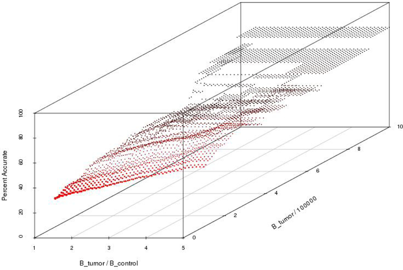
The gene identification accuracy associated with non-parametric bootstrapping. Recall that B_tumor and B_control denote the betweenness value of the tumor and control networks, respectively. Thus, the two planar axes represent the threshold values used in Algorithm 1 associated with the ratio of tumor betweenness to control betweenness, and the (scaled) tumor betweenness. For this graph, these are interpreted as the threshold values used to identify essentially different genes. The graph is generated as follows: For each value on the plane, (B_tumor/B_control, B_tumor × 10⁻⁵), Algorithm 1 is applied with these threshold values, using non-parametric bootstrapping to generate the 100 simulated networks in Step 4. This results in a set of essentially different genes and a set of significantly different genes, from which the accuracy, as defined by Equation (5), is calculated. This accuracy value determines the height of the graph at the given point on the plane.

Fig. 5.

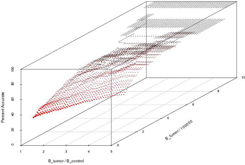
This graph represents the gene identification accuracy for each (B_tumor/B_control, B_tumor × 10⁻⁵) set of threshold values, similar to Figure 4. In this figure, the 100 simulated networks in Step 4 of Algorithm 1 are generated by adding noise to the edge-weights. To each initial edge-weight, r, we add noise with a truncated Normal distribution centered at r with standard deviation given by Equation (4).

4. Application

While our method may be generalized to a variety of networks and centrality measures, we illustrate the variability of betweenness on a specific gene regulatory network. The glioma network was constructed from Rembrandt microarray data (available from GEO GSE68848 [19]), which includes 874 glioma specimens. The network was built from the Rembrandt data using the ARACNe-AP algorithm, as described in [20,21]. The network is publicly available as a supplement to [10].

RNA expression data from pediatric brain tumors (available from GEO GSE42656) were used to create two separate weighted networks, one based on each of the control and tumor sets of samples. The tumor group consists of 14 pilocytic astrocytoma samples, a type of low-grade glioma. The normal group consists of 16 samples from healthy brain tissue. These two datasets were chosen not only because they contained normal (non-neoplastic) tissue for comparison, but also because they allow for comparisons to our previously generated low-grade mouse glioma [10]. Figure 1 illustrates the two data sets as side-by-side heat maps. We emphasize that the network structure was identical for both groups, but the weights assigned to the edges differed. In addition, genes that were not identified in one of the groups were removed from the network.

To generate a set of essentially different genes, we followed the procedure detailed in [10], where a gene was considered essentially different if it had high betweenness centrality. More specifically, a gene was essentially different if it had a tumor betweenness value that was greater than 950,000 and a tumor to control betweenness proportion greater than 1.5. Based upon the results of our sensitivity analysis, as shown in Figures 4 and 5, these thresholding values were appropriate to use in the identification of essentially different genes. For example, in the figures, the graphs are at when the independent variables are increased above (1.5, 950,000), i.e. no increase in accuracy is achieved by raising these thresholds. In other words, the sensitivity analyses show that the results will not change if the thresholds are increased beyond 1.4 for the tumor/control betweenness ratio, or above 910,000 for the tumor betweenness value. The figures are discussed further in the next section. The set of essentially different genes are detailed in Table 3.

Table 3.

The set of essentially different genes identified using only thresholds on betweenness centrality. Recall that ${\widehat{C}}_{B_{\text{tumor}}}$ and ${\widehat{C}}_{B_{\text{control}}}$ are the tumor and control betweenness value, respectively, of the genes in the unperturbed networks.

Gene	${\widehat{C}}_{B_{\text{control}}}$	${\widehat{C}}_{B_{\text{tumor}}}$	${\widehat{C}}_{B_{\text{tumor}}}/{\widehat{C}}_{B_{\text{control}}}$
CEBPB	170000	1130000	6.65
OLIG1	101000	1380000	13.7
SOX8	203000	1250000	6.16
SP100	18700	1120000	59.9
THRA	80600	1550000	19.2

With the initial set of essentially different genes, we were able to analyze the variability of the betweenness difference statistic through two perturbation approaches on the edge-weights: non-parametric bootstrapping and addition of random noise. For each perturbation method, the threshold values were set to those used to identify essentially different genes.

4.1. Perturbation with Non-Parametric Bootstrapping

Resampling with replacement of 14 and 16 samples from the tumor and control data sets, respectively, we constructed 100 bootstrapped tumor and 100 bootstrapped control networks. After applying the confidence interval procedure in Algorithm 1 to samples generated by non-parametric bootstrapping, the results shown in Figure 4 indicated that the highest level of accuracy of 80% was achieved with thresholds of a tumor to control betweenness proportion greater than 1.4 and a tumor betweenness greater than 910,000.

The results of our bootstrapping perturbation method are listed in Table 4. Note that the experimental validation procedure given in [10] is not always feasible, and the perturbation methods in this work have given an alternative way for validating the set of essentially different genes. Indeed, of the 5 essentially different genes originally found using thresholding criteria, only four had confidence intervals that excluded zero.

Table 4.

The set of statistically different genes identified through our confidence interval method using non-parametric bootstrapping. Recall that ${\widehat{D}}_B$ is the difference in tumor and control log betweenness values from the unperturbed networks, and $\overline{\tilde{D}}$ and ${\sigma }_{{\tilde{D}}_B}$ are the mean and standard deviation of the difference in tumor and control log betweenness values of the perturbed networks, respectively.

Gene	${\widehat{D}}_B$	${\overline{\tilde{D}}}_B$	${\sigma }_{{\tilde{D}}_B}$	95% confidence Interval
OLIG1	2.61471	1.9240	0.811	(0.993, 4.2367)
SOX8	1.81769	1.5084	0.861	(0.095, 3.5404)
SP100	4.09251	2.9666	1.326	(1.440, 6.7451)
THRA	2.95650	2.1650	1.140	(0.676, 5.2370)

4.2. Perturbation with Addition of Random Noise

Perturbing the correlation values of each gene-gene pair using a truncated normal distribution, we constructed 100 perturbed simulated tumor and 100 perturbed simulated control networks. Applying the confidence interval procedure in Algorithm 1 to samples generated by adding noise generated from a truncated normal distribution to the correlation values, the highest level of accuracy achieved was 100% with thresholds of a tumor to control betweenness proportion greater than 1.4 and a tumor betweenness greater than 910,000, as in Figure 5.

The results of the random noise perturbation method are listed in Table 5. Using the confidence interval method as an alternative way for validating the set of essentially different genes, all of the 5 essentially different genes had confidence intervals that excluded zero.

Table 5.

The set of statistically different genes identified through our confidence interval method by adding random noise from a truncated normal distribution to the correlation values.

Gene	${\widehat{D}}_B$	${\overline{\tilde{D}}}_B$	${\sigma }_{{\tilde{D}}_B}$	95% confidence Interval
CEBPB	1.89417	1.9276	0.791	(0.3114, 3.477)
OLIG1	2.61471	2.2570	0.961	(0.6929, 4.537)
SOX8	1.81769	2.2344	0.680	(0.4567, 3.179)
SP100	4.09251	3.2332	0.795	(2.5019, 5.683)
THRA	2.95650	2.4985	0.659	(1.6385, 4.274)

Three (CEBPB, OLIG1 and SOX8) of these five genes encode transcription factors. In this regard, CCAAT/Enhancer binding protein beta (CEBPB) belongs to the basic leucine zipper transcription factor family, where it facilitates glioma mesenchymal transition (an indicator of tumor aggressiveness) and correlates with reduced patient survival ([22–24]). Similarly, liver-enriched inhibitory protein (LIP), an isoform of the CEBPB protein, increases glioma cell proliferation and migration, likely by altering the tumor microenvironment [25]. Oligodendrocyte transcription factor 1 (OLIG1) is a transcription factor that induces oligodendrocyte development and remyelination in the central nervous system ([26, 27]). Increased OLIG1 expression has been reported in brain tumors, including oligodendroglioma ([28, 29]). SOX8 belongs to the SOX (SRY-related HMG-box) family of transcription factors, where its ectopic expression increases hepatocellular carcinoma cell proliferation [30]. In addition, SOX8 has been implicated in chemoresistance, stemness, and mesenchymal transition of tongue squamous cell carcinoma [31]. It is worth noting that SOX8 expression is elevated in low-grade astrocytomas [32]. SP100 nuclear antigen (SP100) encodes a nuclear antigen covalently modified by the SUMO-1 modifier. SP100A (one SP100 isoform) stabilizes the transactivation of p53, a tumor suppressor [33] and activates ETS-1, a transcription factor involved in glioma formation ([34, 35]). Thyroid hormone receptor, alpha (THRA) functions as a receptor for thyroid hormones, which have growth promoting effects on glioma cells [36]. While the roles of these five essentially different genes in pilocytic astrocytoma remain to be explored, the methodology described herein resulted in the identification of genes and gene networks worthy of future study.

5. Discussion

In our application, we created two separate weighted networks based upon each of the control and tumor sets of samples from pediatric low-grade brain tumors (pilocytic astrocytoma), where the edge-weights were assigned using correlations between genes. These datasets were specifically chosen based on the availability of non-neoplastic control tissue samples and our previous studies focused on low-grade gliomas arising in murine models of Neurofibromatosis type 1 (NF1) [10]. We used the betweenness centrality measure to identify a set of essentially different genes whose role had substantially changed in the comparison of healthy to diseased states. To address the variability of the betweenness statistic in the comparison of two networks, we proposed a theoretical framework to construct confidence intervals on the estimated betweenness difference measures. If an essentially different gene had a confidence interval that excluded zero, then that gene was determined to be statistically different across the tumor and healthy networks. To simulate the distribution of the betweenness difference measure, we utilized two separate edge-weight perturbation methods: non-parametric bootstrapping and the addition of random noise to each gene-gene pair correlation. Although both perturbation methods confirmed four of the five essentially different genes as statistically different, the fifth gene was identified only through the addition of random noise. While it is important to note that our work relies on a given network structure considered to be fixed (a gene regulatory network from [20] was used in the application, but any relevant base network could be used for a given problem), the results of our proposed framework, assessed with two distinct edge-weight perturbation methods, suggest a general robustness of betweenness centrality when used as a method for identifying genes essential to a biological network.

Previous work used thresholding to find essential genes, i.e. genes that are essentially different in comparing networks derived from tumor samples as compared to networks from healthy samples. That work can be experimentally validated in the laboratory. Our work allows for computational validation in situations where experiments are not feasible. In particular, by bootstrapping and perturbing edge-weights with random noise, we are able to identify genes that are both essentially different and significantly different across the two networks. The analysis has applications to any fixed network structure with edge-weights that change across conditions. We also note that, in some situations, we might want to identify genes whose centrality is repressed in the tumor. This could be accomplished using the same methodology that we present here, with the roles of B_tumor and B_control reversed.

In order to integrate our method with drug discovery, we briefly describe the next steps in the validation process. Following the identification of a candidate gene or set of genes, the observed differential in betweenness should be validated using an independent set of samples. These validation studies may involve analyses at the RNA level (RNA sequencing, quantitative real-time polymerase chain reaction and uorescent in situ hybridization), protein level (immunoblotting, proteomics, and immunohistochemistry), or activity level using reagents that recognize secondary protein modifications (e.g., phosphorylation). In addition, publically available databases (e.g., Gene Expression Omnibus, The Cancer Genome Atlas, Cancer Cell Line Encyclopedia, Human Protein Atlas, and Genotype-Tissue Expression Database) can be used to determine whether differential betweenness of the gene(s) is conserved across multiple data sets. This will help determine whether the observed gene signature is shared by the majority of the disease samples or is restricted to certain conditions/disease subsets.

After initial validation studies have been completed, mechanistic studies usually ensue, in which the functional relationships between the gene(s) in question and the related disease state are experimentally evaluated in model systems or experimental platforms (e.g., cell lines, mouse models, or human tumor xenografts). In the situation where a specific gene is over-expressed in cancer relative to normal tissue, genetic (CRISPR/Cas9 editing or short hairpin RNA) or pharmacological inhibition of that protein is used to determine whether its silencing attenuates some aspects of tumor biology (e.g., tumor growth or metastasis). When a gene is reduced or mutated in cancer compared to its corresponding normal counterpart, the gene can be re-introduced (by DNA transfection or viral delivery) or the mutation corrected by CRISPR/Cas9 editing. These lines of investigation can involve both in vitro (cell culture) and in vivo (live animal) approaches, as well as the use of genetically-engineered mouse models, each yielding different insights into the role of that specific gene in disease pathogenesis. To determine whether a network of genes function in a collective manner, their hierarchical dependence can be established using the above methods, and their individual contributions defined by normalizing combinations of the identified genes.

To illustrate this forward flow, consider an earlier study that only used expression levels [37]. differential RNA expression analysis of malignant mouse sarcoma cancer cell lines revealed that expression of the CXCR4 chemokine receptor was increased relative to the normal control cell lines. This in silico finding was then validated at the RNA (quantitative real-time polymerase chain reaction) and protein (immunoblotting) levels. These findings were extended to human cancers by demonstrating increased CXCR4 protein expression in the majority of surgical specimens analyzed. To demonstrate that CXCR4 controls sarcoma growth, CXCR4 levels were reduced in the cancer cells using short hairpin RNA interference, resulting in decreased tumor growth in vitro and in vivo. Lastly, to evaluate the potential of CXCR4 as a drug target for treating these cancers, a CXCR4 inhibitor, AMD3100 was used to demonstrate its ability to attenuate cancer cell proliferation in vitro and tumor growth in mice in vivo.

Similarly, we employed RNA sequencing of microglia isolated from Nf1 mouse optic glioma tumors to identify a stromal growth factor, Ccl5, uniquely overexpressed in these immune system-like cells relative to their normal counterparts [38]. This differential expression was subsequently validated at the RNA and protein levels, and Ccl5 was shown to increase Nf1 optic glioma cell growth in vitro. Importantly, blocking Ccl5 function in mice with optic gliomas dramatically inhibited tumor growth in vivo, suggesting that Ccl5 might be a critical growth factor for brain tumors. Subsequent studies demonstrated that Ccl5 was also important for malignant glioma growth in vitro and in vivo [39].

Indeed, it is plausible to use differential betweenness in lieu of differential expression as a more complex measure of the changes in gene relationships for different cell states. Follow-up validation could lead to important and nuanced information for drug targeting.

References

- 1.del Rio G, Koschützki D, and Coello G, “How to identify essential genes from molecular networks?,” BMC Systems Biology, vol. 3, no. 1, p. 102, 2009. [DOI] [PMC free article] [PubMed] [Google Scholar]
- 2.Han J-DJ, Bertin N, Hao T, Goldberg DS, Berriz GF, Zhang LV, Dupuy D, Walhout AJ, Cusick ME, Roth FP, et al. , “Evidence for dynamically organized modularity in the yeast protein–protein interaction network,” Nature, vol. 430, no. 6995, p. 88, 2004. [DOI] [PubMed] [Google Scholar]
- 3.Vallabhajosyula RR, Chakravarti D, Lutfeali S, Ray A, and Raval A, “Identifying hubs in protein interaction networks,” PLoS ONE, vol. 4, no. 4, p. e5344, 2009. [DOI] [PMC free article] [PubMed] [Google Scholar]
- 4.Jeong H, Mason SP, Barabási A-L, and Oltvai ZN, “Lethality and centrality in protein networks,” Nature, vol. 411, no. 6833, p. 41, 2001. [DOI] [PubMed] [Google Scholar]
- 5.Freeman LC, “A set of measures of centrality based on betweenness,” Sociometry, pp. 35–41, 1977.
- 6.Bavelas A, “Communication patterns in task-oriented groups,” The Journal of the Acoustical Society of America, vol. 22, no. 6, pp. 725–730, 1950. [Google Scholar]
- 7.Bonacich P, “Power and centrality: A family of measures,” American Journal of Sociology, vol. 92, no. 5, pp. 1170–1182, 1987. [Google Scholar]
- 8.Li M, Wang J, Chen X, Wang H, and Pan Y, “A local average connectivity-based method for identifying essential proteins from the network level,” Computational Biology and Chemistry, vol. 35, no. 3, pp. 143–150, 2011. [DOI] [PubMed] [Google Scholar]
- 9.Tang X, Wang J, Zhong J, and Pan Y, “Predicting essential proteins based on weighted degree centrality,” IEEE/ACM Transactions on Computational Biology and Bioinformatics (TCBB), vol. 11, no. 2, pp. 407–418, 2014. [DOI] [PubMed] [Google Scholar]
- 10.Pan Y, Duron C, Bush EC, Ma Y, Sims PA, Gutmann DH, Radunskaya A, and Hardin J, “Graph complexity analysis identifies an ETV5 tumor-specific network in human and murine low-grade glioma,” PLoS ONE, 13 (5): e0190001. [DOI] [PMC free article] [PubMed] [Google Scholar]
- 11.Breitkreutz D, Hlatky L, Rietman E, and Tuszynski J, “Molecular signaling network complexity is correlated with cancer patient survivability,” Proceedings of the National Academy of Sciences, vol. 109, no. 23, pp. 9209–9212, 2012. [DOI] [PMC free article] [PubMed] [Google Scholar]
- 12.Ramadan E, Alinsaif S, and Hassan MR, “Network topology measures for identifying disease-gene association in breast cancer,” BMC Bioinformatics, vol. 17, no. 7, p. 274, 2016. [DOI] [PMC free article] [PubMed] [Google Scholar]
- 13.Zhang X, Xu J, and Xiao W, “A new method for the discovery of essential proteins,” PLoS ONE, vol. 8, no. 3, p. e58763, 2013. [DOI] [PMC free article] [PubMed] [Google Scholar]
- 14.Mistry D, Wise RP, and Dickerson JA, “DiffSLC: A graph centrality method to detect essential proteins of a protein-protein interaction network,” PLoS ONE, vol. 12, no. 11, p. e0187091, 2017. [DOI] [PMC free article] [PubMed] [Google Scholar]
- 15.Segarra S and Ribeiro A, “Stability and continuity of centrality measures in weighted graphs,” IEEE Transactions on Signal Processing, vol. 64, no. 3, pp. 543–555, 2016. [Google Scholar]
- 16.Epskamp S, Borsboom D, and Fried EI, “Estimating psychological networks and their accuracy: A tutorial paper,” Behavior Research Methods, pp. 1–18, 2017. [DOI] [PMC free article] [PubMed]
- 17.Boccaletti S, Latora V, Moreno Y, Chavez M, and Hwang D-U, “Complex networks: Structure and dynamics,” Physics Reports, vol. 424, no. 4–5, pp. 175–308, 2006. [Google Scholar]
- 18.Newman ME, “The structure and function of complex networks,” SIAM Review, vol. 45, no. 2, pp. 167–256, 2003. [Google Scholar]
- 19.Madhavan S, Zenklusen J-C, Kotliarov Y, Sahni H, Fine HA, and Buetow K, “Rembrandt: helping personalized medicine become a reality through integrative translational research,” Molecular Cancer Research, vol. 7, no. 2, pp. 157–167, 2009. [DOI] [PMC free article] [PubMed] [Google Scholar]
- 20.Margolin AA, Nemenman I, Basso K, Wiggins C, Stolovitzky G, Dalla Favera R, and Califano A, “ARACNE: an algorithm for the reconstruction of gene regulatory networks in a mammalian cellular context,” in BMC Bioinformatics, vol. 7, p. S7, 2006. [DOI] [PMC free article] [PubMed] [Google Scholar]
- 21.Lachmann A, Giorgi FM, Lopez G, and Califano A, “ARACNe-AP: gene network reverse engineering through adaptive partitioning inference of mutual information,” Bioinformatics, vol. 32, no. 14, pp. 2233–2235, 2016. [DOI] [PMC free article] [PubMed] [Google Scholar]
- 22.Yin J, Oh Y, Kim J, Kim S, Choi E, Kim T, Hong J, Chang N, Cho H, Sa J, Kim J, Kwon H, Park S, Lin W, Nakano I, Gwak H, Yoo H, Lee S, Lee J, Kim J, Kim S, Nam D, Park M, and Park J, “Transglutaminase 2 inhibition reverses mesenchymal transdifferentiation of glioma stem cells by regulating C/EPBβ signaling,” Cancer Research, vol. 77, pp. 4973–4984, September 2017. [DOI] [PubMed] [Google Scholar]
- 23.Carro MS, Lim WK, Alvarez MJ, Bollo RJ, Zhao X, Snyder EY, Sulman EP, Anne SL, Doetsch F, Colman H, Lasorella A, Aldape K,Califano A, and Iavaone A, “The transcriptional network for mesenchymal transformation of brain tumours,” Nature, vol. 463, pp. 318–325, January 2010. [DOI] [PMC free article] [PubMed] [Google Scholar]
- 24.Cooper LAD, Gutman DA, Chisolm C, Appin C, Kong J, Rong Y, Kurc T, Van Meir EG, Saltz JH, Moreno CS, and Brat DJ, “The tumor microenvironment strongly impacts master transcriptional regulators and gene expression class of glioblastoma.,” The American Journal of Pathology, vol. 180, no. 5, pp. 2108–2119, 2012. [DOI] [PMC free article] [PubMed] [Google Scholar]
- 25.Selagea L, Mishra A, Anand M, Ross J, Tucker-Burden C, Kong J, and Brat DJ, “EGFR and C/EBP-β oncogenic signaling is bidirectional in human glioma and varies with the C/EBP-β isoform,” FASEB, vol. 30, pp. 4098– 4108, December 2016. [DOI] [PMC free article] [PubMed] [Google Scholar]
- 26.Sabo JK, Heine V, Silbereis JC, Schirmer L, Levison SW, and Rowitch DH, “Olig1 is required for noggin-induced neonatal myelin repair,” Annals of Neurology, vol. 81, pp. 560–571, April 2017. [DOI] [PMC free article] [PubMed] [Google Scholar]
- 27.Motizuki M, Isogaya K, Miyake K, Ikushima H, Kubota T, Miyazono K, Saitoh M, and Miyazawa K, “Oligodendrocyte transcription factor 1 (Olig1) is a smad cofactor involved in cell motility induced by transforming growth factor-β,” Journal of Biological Chemistry, vol. 288, pp. 18911–18922, June 28 2013. [DOI] [PMC free article] [PubMed] [Google Scholar]
- 28.Jakovcevski I and Zecevic N, “Olig transcription factors are expressed in oligodendrocyte and neuronal cells in human fetal CNS,” Journal of Neuroscience, vol. 25, pp. 10064–10073, November 2 2005. [DOI] [PMC free article] [PubMed] [Google Scholar]
- 29.Azzarelli B, Miravalle L, and Vidal R, “Immunolocalization of the oligo-dendrocyte transcription factor 1 (Olig1) in brain tumors,” Journal of Neuropathology and Experimental Neurology, vol. 63, pp. 170–179, February 2004. [DOI] [PubMed] [Google Scholar]
- 30.Zhang S, Zhu C, Zhu L, Liu H, Liu S, Zhao N, Wu J, Huang X, Zhang Y, Jin J, Ji T, and Ding X, “Oncogenicity of the transcription factor SOX8 in hepatocellular carcinoma,” Medical Oncology, vol. 31, April 2014. [DOI] [PubMed] [Google Scholar]
- 31.Xie SL, Fan S, Zhang SY, Chen WX, Li QX, Pan GK, Zhang HQ, Wang WW, Weng B, Zhang Z, Li JS, and Lin ZY, “SOX8 regulates cancer stem-like properties and cisplatin-induced EMT in tongue squamous cell carcinoma by acting on the Wntβ-catenin pathway,” International Journal of Cancer, vol. 142, pp. 1252–1265, March 15 2018. [DOI] [PubMed] [Google Scholar]
- 32.Schlierf B, Friedrich RP, Roerig P, Felsberg J, Reifenberger G, and Wegner M, “Expression of SoxE and SoxD genes in human gliomas,” Neuropathology and Applied Neurobiology, vol. 33, pp. 621–630, December 2007. [DOI] [PubMed] [Google Scholar]
- 33.Berscheminski J, Brun J, Speiseder T, Wimmer P, Ip WH, Terzic M, Dobner T, and Schreiner S, “Sp100A is a tumor suppressor that activates p53-dependent transcription and counteracts E1A/E1B-55K-mediated transformation,” Oncogene, vol. 35, pp. 3178–3189, June 16 2016. [DOI] [PubMed] [Google Scholar]
- 34.Wasylyk C, Schlumberger S, Criqui-Filipe P, and Wasylyk B, “Sp100 interacts with ETS-1 and stimulates its transcriptional activity,” Molecular and Cellular Biology, vol. 22, pp. 2687–2702, April 2002. [DOI] [PMC free article] [PubMed] [Google Scholar]
- 35.Sahin A, Velten M, Pietsch T, Knuefermann P, Okuducu A, Hahne J, and Wernert N, “Inactivation of Ets 1 transcription factor by a specific decoy strategy reduces rat C6 glioma cell proliferation and mmp-9 expression,” International Journal of Molecular Medicine, vol. 15, pp. 771–776, May 2005. [PubMed] [Google Scholar]
- 36.Davis FB, Tang H-Y, Shih A, Keating T, Lansing L, Hercbergs A, Fenstermaker RA, Mousa A, Mousa SA, Davis PJ, and Lin H-Y, “Acting via a cell surface receptor, thyroid hormone is a growth factor for glioma cells,” Cancer Research, vol. 66, pp. 7270–7275, July 15 2006. [DOI] [PubMed] [Google Scholar]
- 37.Mo W, Chen J, Patel A, Zhang L, Chau V, Li Y, Cho W, Lim K, Xu J, Lazar AJ, et al. , “CXCR4/CXCL12 mediate autocrine cell-cycle progression in NF1-associated malignant peripheral nerve sheath tumors,” Cell, vol. 152, no. 5, pp. 1077–1090, 2013. [DOI] [PMC free article] [PubMed] [Google Scholar]
- 38.Solga AC, Pong WW, Kim K-Y, Cimino PJ, Toonen JA, Walker J, Wylie T, Magrini V, Griffith M, Griffith OL, et al. , “RNA sequencing of tumor-associated microglia reveals Ccl5 as a stromal chemokine critical for neurofibromatosis-1 glioma growth,” Neoplasia, vol. 17, no. 10, pp. 776–788, 2015. [DOI] [PMC free article] [PubMed] [Google Scholar]
- 39.Pan Y, Smithson LJ, Ma Y, Hambardzumyan D, and Gutmann DH, “Ccl5 establishes an autocrine high-grade glioma growth regulatory circuit critical for mesenchymal glioblastoma survival,” Oncotarget, vol. 8, pp. 32977– 32989, May 2017. [DOI] [PMC free article] [PubMed] [Google Scholar]