Development of a protein–ligand extended connectivity (PLEC) fingerprint and its application for binding affinity predictions

Abstract

Motivation

Fingerprints (FPs) are the most common small molecule representation in cheminformatics. There are a wide variety of FPs, and the Extended Connectivity Fingerprint (ECFP) is one of the best-suited for general applications. Despite the overall FP abundance, only a few FPs represent the 3D structure of the molecule, and hardly any encode protein–ligand interactions.

Results

Here, we present a Protein–Ligand Extended Connectivity (PLEC) FP that implicitly encodes protein–ligand interactions by pairing the ECFP environments from the ligand and the protein. PLEC FPs were used to construct different machine learning models tailored for predicting protein–ligand affinities (pK_i∕d). Even the simplest linear model built on the PLEC FP achieved R_p = 0.817 on the Protein Databank (PDB) bind v2016 ‘core set’, demonstrating its descriptive power.

Availability and implementation

The PLEC FP has been implemented in the Open Drug Discovery Toolkit (https://github.com/oddt/oddt).

Supplementary information

Supplementary data are available at Bioinformatics online.

1 Introduction

Fingerprints (FPs) are one of the key concepts in cheminformatics, allowing for effective representation of a molecule with a fixed length vector of Booleans or integers. Such representations are highly efficient to process, store and compare. There are a wide variety of FP flavours, from the most simplistic, enumerating a catalogue of 2D substructures (e.g. MACCS), to more advanced versions that enclose 3D information about the molecular conformation (Axen et al., 2017).

The Extended Connectivity Fingerprint (ECFP) is one of the most versatile types of FP for general use (Maggiora et al., 2014; O’Boyle and Sayle, 2016). ECFPs store information about the environments surrounding each atom in a molecule (Rogers and Hahn, 2010). The environments are defined by the bond-step radius, e.g. ECFP1 encodes the root atom and its direct neighbours. This FP has already been successfully used as an input to train machine learning (ML) models in ligand-based virtual screening (Chen et al., 2012).

FPs have also been used to represent intramolecular interactions. Structural Interaction Fingerprints (SiFTs) (Deng et al., 2004) and Python-based Protein–Ligand Interaction Fingerprints (PyPLIFs) (Radifar et al., 2013) explicitly define well-known interaction types such as hydrogen bonds, halogen bonds and π stacking and map them onto the protein sequence. There are also variants of interaction fingerprints (IFPs) that group interactions by the residue type, e.g. the Simple Ligand–Receptor Interaction Descriptor (SILIRID) (Chupakhin et al., 2014). A more advanced IFP, the Structural Protein–Ligand Interaction Fingerprint (SPLIF) (Da and Kireev, 2014), uses an ECFP atom hashing algorithm instead of explicit definitions of the interactions. Here, ECFP1, accompanied by the Cartesian coordinates of the atoms, is used to represent contacts. To select similar ligand poses within a complex, a custom similarity function is used that accounts for the 3D distance during bits matching. There have also been some efforts to include the protein environment in this type of FP. In LORD_FP (Weber et al., 2015), the receptor environment is encoded using the pharmacophoric types of protein atoms within a certain distance of the ligand atoms (2, 3 and 4.5 Å bins).

Efforts have been made to use IFPs in scoring functions (SF) to predict binding affinities with the assistance of ML models, such as neural networks (Chupakhin et al., 2013; Gomes et al., 2017; Vass et al., 2016; Witek et al., 2014), random forest (Sato et al., 2010) and support vector machines (Yan et al., 2017). The SPLIF FPs were recently integrated into the MoleculeNet benchmark (Wu et al., 2017), which yielded promising results when trained on Protein Databank (PDB) bind database.

Although a number of attempts have been made to develop interaction FPs, we still lack a general, descriptive and versatile solution that is useful as an input for training SF and other predictive models. Herein, we describe a Protein–Ligand Extended Connectivity (PLEC) FP, a novel IFP that encodes the ECFP environments of the protein and the ligand atoms in contact, and demonstrate its application to binding affinity predictions. Various ML models have been trained with PLEC, all showing similar, consistent results, superior to SILIRID (Chupakhin et al., 2014), SPLIF (Da and Kireev, 2014), RF-Score v3 (Li et al., 2015) and X-Score (Wang et al., 2002). These results emphasize the ‘scoring power’ of PLEC FPs, as introduced by CASF benchmark (Li et al., 2014), with the ‘screening’ and ‘docking’ powers yet to be optimized in future research. Our results suggest, that the implicit approach to defining protein–ligand interactions allows for PLEC to be used in other areas such as lead optimization and scaffold hopping campaigns.

2 Materials and methods

2.1 Fingerprint construction

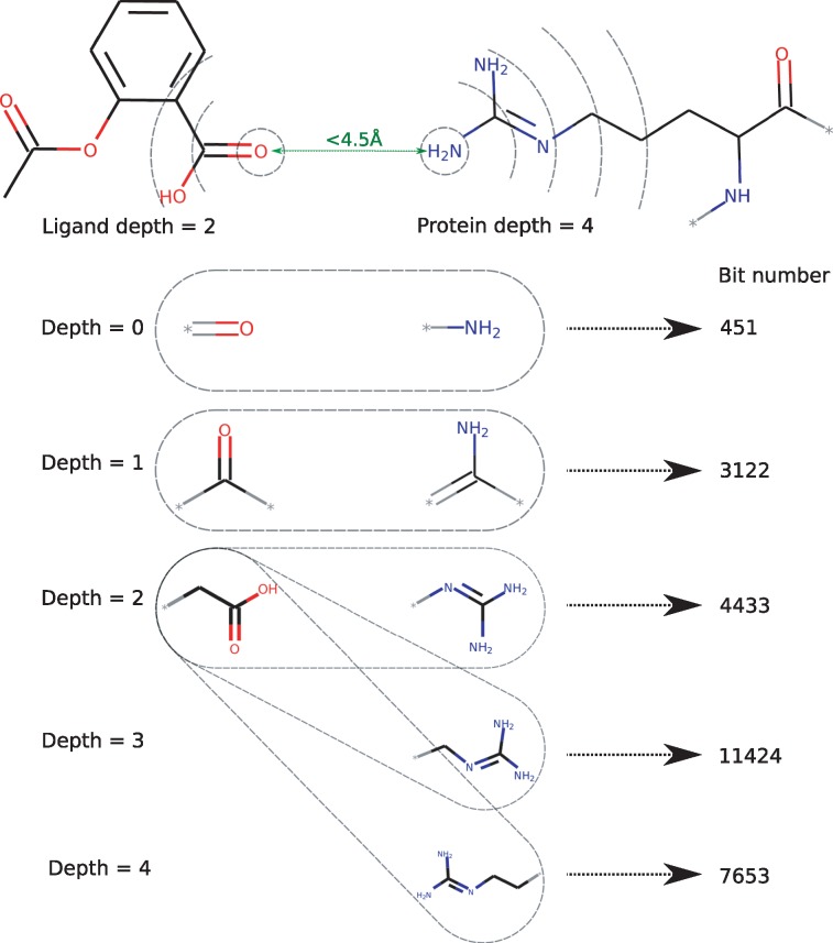
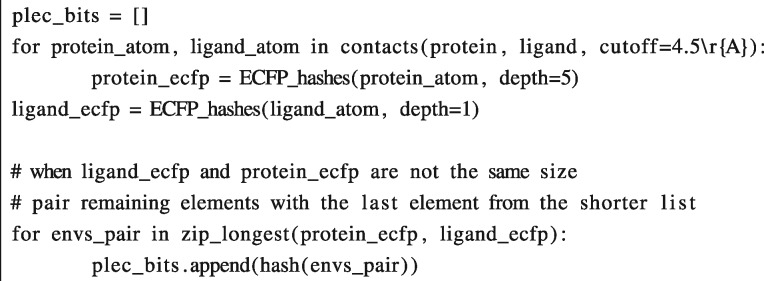
The PLEC FP builds on the idea of atom environments originally presented by Rogers and Hahn (2010) in the ECFP. The atomic features are identical to those in ECFP, i.e. the atomic number, isotope, number of neighbouring heavy atoms, number of hydrogens, formal charge, ring membership and aromaticity. However, in contrast to ECFP, only atoms in contact with another molecule are used in the PLEC FP. The algorithm (see pseudocode below) consists of two main steps. First, for a pair of interacting atoms, defined by default as within a 4.5 Å distance cut-off (in 3D space), the environments are identified for each atom. An environment contains the root atom itself and its closest neighbours, within at most n bonds diameter (defined by the ‘depth’ parameter), see Figure 1. Note that the environment, which is meant to describe physico-chemical properties of a root atom, is based on a molecule’s topology only and does not include any 3D information. During the second step, each ligand environment is paired with an environment of corresponding depth from the receptor, and these pairings are subsequently hashed to a final bit position in the PLEC FP. If one of the molecules has greater depth (as shown in Fig. 1), the additional environments are paired with the largest environment from the other molecule. Water molecules can also be included, as the water-bridged interactions may play an important role in molecule binding. In these cases, the water molecules are attributed to the receptor. During our analysis we have ignored water molecules, since modelling their explicit positions in an automated manner would be prone to error.

Fig. 1.

Construction of the PLEC fingerprint. Depicted is the schematic 2D representation of a 3D complex. Atoms in close contact (green) are identified, followed by the subsequent generation and hashing of corresponding layers on the ligand and the protein side. Note that the ligand depth is 2 and the receptor depth is 4

PLEC uses a standard Python hashing function ‘hash’, modified to produce an unsigned 32-bit integer. The raw FP consists of integers between 0 and 2³² (32 bits) and is folded, as in every other FP, to a much smaller length. We have analysed different folding sizes of FPs, ranging from 2¹² to 2¹⁶, to assess the performance of various models.

Algorithm pseudocode:

Tanimoto or Dice coefficients [similarity measures for binary and count vectors, widely used in cheminformatics (Maggiora et al., 2014)] can be used to compare two PLEC FPs, in the same way that standard FPs are compared. As the PLEC FP is invariant to orientation in 3D space, complexes do not need to be aligned to compare two different ligand poses. Due to the implicit enumeration of the interactions in the PLEC FP, which does not encode the protein sequence, receptor–ligand complexes formed by proteins with different sequences can be compared to each other.

2.2 Machine learning models

Scikit-learn was used as a prime ML python library, which was proven to be performant and robust (Pedregosa et al., 2011). Three types of ML models were built in scikit-learn v. 0.19 and trained using the PLEC FP to predict protein–ligand affinities (pK_i∕d), specifically:

• linear regression (SGDRegressor);

• random forest (RandomForestRegressor);

• neural network (MLPRegressor);

The linear model used the Huber loss and the ‘elasticnet’ penalty as elements of the objective function. Huber loss is a hybrid loss function, which uses a mixture of quadratic cost for small errors and linear cost for less accurate predictions, enhancing handling of outliers when compared to standard quadratic cost, see Equation (1) (Huber, 1964).

$$\begin{array}{c}{L}_{\delta }(y,f(x))=\{\begin{array}{cc}\frac{1}{2}{(y-f(x))}^2\hfill & \text{for} |y-f(x)|\le \delta ,\hfill \\ \delta |y-f(x)|-\frac{1}{2}{\delta }^2\hfill & \text{otherwise}.\hfill \end{array}\end{array}$$ (1)

$$\begin{array}{c}\text{Equation}\hspace{0.17em}1:\text{Huber}\hspace{0.17em}\text{loss}\hspace{0.17em}\text{objective}\hspace{0.17em}\text{function}\hspace{0.17em}\text{equation}.\end{array}$$

‘Elasticnet’ penalty, similarly to Huber loss, is also a hybrid penalty function that applies L2 (quadratic) penalty to certain cut-off ($ϵ=0.1$) and L1 (linear) penalty for others to keep the coefficients low. Random forest was built with 100 fully grown trees; neither the depth nor the number of leaf limits were specified. A dense, also called fully connected feed-forward, neural network with 3 hidden layers of 200 neurons each was built using MLPRegressor. All the neurons had ReLU activations [Rectified Linear Unit, which is a positive part of an input—$\text{max}(0,x)$] and the network was trained with L-BFGS-B minimization. We have also tried various dense networks implemented in TensorFlow (Abadi et al., 2016), but the results were very similar to the scikit-learn implementation and did not improve with increasing network complexity (data not shown).

2.3 Training and testing datasets

PDBbind v2016 (Liu et al., 2017) was used for training and testing the predictive models built with the PLEC FP. The PDBBind dataset consist of receptor–ligand complexes, with experimentally determined 3D structures and binding affinity values. It is divided into three overlapping subsets: general, refined and core set. Usually the ‘refined set’, consisting of 3673 complexes, is utilized for training predictive models, whereas the ‘core set’ (295 complexes) is used for testing whether those predictions are valid (Li et al., 2014, 2015; Zilian and Sotriffer, 2013). In our work we have explored the relationship between the size of the training set and the performance of the PLEC linear model, to be sure enough data is available for training (see Supplementary Fig. S1). Our analysis showed that the ‘refined set’ far too small for this purpose as the linear model generalized poorly. Therefore, we have decided to use the ‘general set’ instead, which consists of 12 906 complexes to train the PLEC based predictive models.

The model benchmarking (testing) was done with two separate ‘core sets’ from PDBbind v2016 and v2013. Note that these sets have an overlap of 108 structures but were evaluated separately for retrospective (e.g. CASF-2013 uses ‘core set’ v2013) and prospective comparisons. As the complexes from training ‘general set’ and testing ‘core sets’ do overlap, it is important to highlight that all overlapping structures were removed from the ‘general set’ to avoid data leakage.

As an additional, external dataset The Astex Diverse Set, consisting of 85 complexes, was used. Similar to the above procedure, all overlapping complexes were removed from the training dataset (the PDBBind v2016 ‘general set’). Additionally, 11 out of the 85 complexes had no binding affinity information, therefore only 74 proteins were used. The only pre-processing applied to the protein files from the Astex dataset was the changing of the mol2 dummy atoms (‘Du’) to appropriate atom types based on their atom labels and residue types.

3 Results and discussion

3.1 Selection of parameters

The PLEC FP is mainly defined by three parameters: the protein depth, the ligand depth and the folded FP size. The values of these three parameters strongly affect the final performance of the predictive models trained on the FP. To find the best set of parameters we have tested protein depths between 1 and 6, ligand depths between 1 and 6 and FP sizes of 4096 (2¹²), 16 384 (2¹⁴), 32 768 (2¹⁵) and 65 536 (2¹⁶). Each of the 144 (6 × 6 × 4) combinations of parameters was fed to three different predictive models (linear regression, random forest and neural network), resulting in 432 distinct models in total. Based on these analyses, we have selected a protein depth of 5, a ligand depth of 1 and a FP size of 65 536 as the most universal set of parameters, with good FP properties and consistent performance across different ML models. Below we provide some of the details of our analysis and the conclusions drawn from them.

3.2 Fingerprint sparsity analysis

To be descriptive, a FP should have very few bits that are either very frequent or very rare. Importantly, high bit occupancy might also be related to collisions that arise due to FP folding (i.e. when two distinct bits are folded to one bit in the final FP). To analyse the sparsity, or the PLEC FP bits occupancy, we have checked how many frequent bits (i.e. interaction types) are present in the PDBbind v2016 ‘general set’. To do this, we have filtered out the bits with a variance threshold of 0.01, which in a count vector such as the PLEC FP translate to a singular difference at certain position for at least 1% of all complexes. Figure 2 shows a saturation plot for different FP sizes from 1024 to 262 144 with depths of 5 and 1 for the protein and the ligand, respectively. For sizes equal to or below 16 384 all the bits are frequent and there is an abundance of collisions. For the size of 65 536 the number of bits reaches a plateau and actually decreases with further elongation of the FPs due to fewer collisions. We observed similar results for other FP depths (see Supplementary Fig. S2). In general, FPs with greater depths require larger sizes as a single contact is described by more bits. A final FP size of 65 536 has been chosen as the most comprehensive option for training predictive models.

Fig. 2.

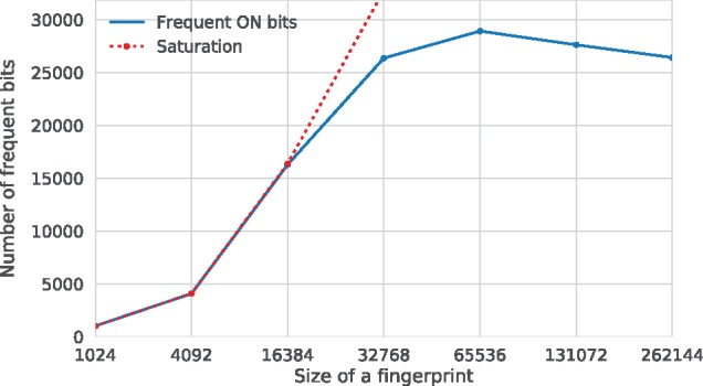
Fingerprint bits saturation plot. The depths of the PLEC FP are 5 and 1 for the protein and the ligand, respectively. For convenience, the fingerprint sizes are plotted on a logarithmic scale. The saturation line (dotted red) shows that all the bits are frequent. Unsaturated FPs are available for sizes larger than 16 384

3.3 Fingerprint depth analysis

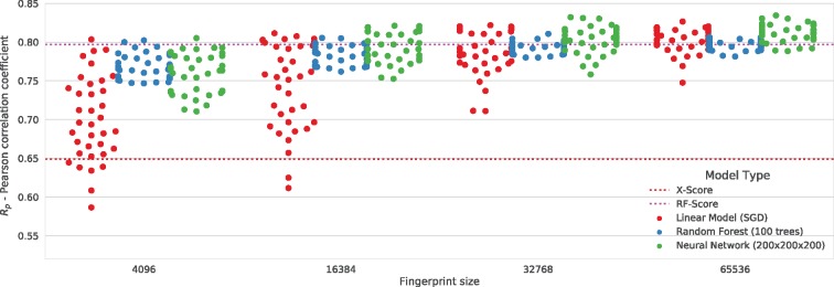
Parameters defining the depths of the protein and the ligand interaction environments have a profound impact on the PLEC FP performance. To establish the most flexible, robust and consistent settings, we have tested each combination (depths ranging from 1 to 6 for the ligand and the receptor, thus 36 combinations) with three different ML models (see Section 2) and four FP sizes. All the models were trained on the PDBbind v2016 ‘general set’ and tested on a non-overlapping ‘core set’. Figure 3 presents the results obtained from this experiment.

Fig. 3.

Prediction accuracy for different combinations of PLEC depth parameters. Each dot depicts the result obtained for a particular combination of a model and fingerprint parameters. Three model types (linear model: red dots, random forest: blue dots and neural network: green dots) were tested against 36 depth combinations for the ligand and the protein (ranges of 1–6; 36 dots for each model) with respect to four fingerprint sizes. The position of each dot on the Y-axis represents the Pearson correlation coefficient (R_p) for the PDBbind ‘core set’ v2016. Red and magenta dotted lines show the results achieved by X-Score (R_p = 0.649) and RF-score v3 (R_p = 0.797, ODDT implementation), respectively

For each of the 36 combinations, a predictive model has been trained and a Pearson correlation coefficient (between the predicted and the measured binding affinity) was plotted as a single coloured dot. Different colours represent different model types, so for each model type and FP size there are 36 dots. The results obtained are shown with respect to FP size (see below). The full set of results is available in Supplementary Table S1.

An important conclusion that can be drawn from the models trained on the PLEC FP is that the performance of nearly every test case is similar, especially when the FP size is larger, even for the least complex, linear model. This consistent predictive power for all the models may be due to the features embodied in PLEC rather than the model complexity. Although a performance gain is possible, especially for shorter FP sizes, by switching from a linear to a more complex model such as random forest or neural network, our results show that the linear regression is preferred due to its simplicity and the direct interpretability of its feature weights. The linear equation coefficients can show the impact of a given feature on the ligand affinity. Importantly, each bit can be traced to a parent substructure, which expands the many possible applications of the PLEC FP.

By weighing the combination of the Pearson correlation coefficients for both the v2016 and v2013 ‘core sets’, we estimated the best-performing size for the PLEC FP to be 65 536 bits. This estimate is also consistent with our sparsity analysis (see Section 3.2).

Finally, from the obtained 432 Pearson correlation coefficients, we also estimated the most consistently performing depths for the PLEC FP, a protein depth of 5 and a ligand depth of 1. A larger protein depth improved the performance of the models, probably due to the additional ability to encode contacts on a residue/side chain level. However, in the case of the ligand, increasing the depth did not improve the overall predictive performance of the models (see Supplementary Table S1). Therefore, we conclude that the nearby environments of the ligand atoms involved in contacts combined with a larger receptor environment provides just enough information for the accurate prediction of affinities.

3.4 Stability of the results

The PDBbind database provides a set of heterogeneous examples of protein–ligand complexes. Usually, models are trained on large sets (i.e. ‘refined’ or ‘general’ sets) and tested on a much smaller ‘core set’ (only 290 structures in v2016). This small test set size can lead to incorrect performance estimates for prospective predictive models. To evaluate the stability of our results, we have tested all the models with 10-fold cross validation (CV). PDBbind contains some redundant proteins, therefore special effort was made during splitting the folds in CV, so that same protein (Uniprot ID) was not shared across testing and training folds. Additionally, an external validation was carried out using the Astex Diverse Set—a set of independently processed, high quality PDB structures.

Each fold in the 10-fold CV contains 1285 or 1286 structures (the total number of complexes is not divisible by 10). In this scenario, the model is tested on a single fold and trained on the remaining complexes.

The Pearson correlation coefficients for CV folds are presented in Figure 4. Not surprisingly, the prediction accuracy depends strongly on the size of the training set. In our CV setup, one-tenth of the samples were moved from the training set to the test set, which lowered the R_p to a reasonable range; in most cases, the R_p values were 0.6–0.7 (Fig. 4A). The linear model was most sensitive to the training size, with particularly high prediction deterioration for smaller FP sizes. The more complex methods, i.e. random forest and neural network, performed more similarly, independent of the number of bits in the FP.

Fig. 4.

Stability of the predictions based on PLEC. (A) Mean performance results (R_p) in 10-fold cross validation for all the tested combinations of PLEC parameters. Each dot depicts the result obtained for a particular combination of a model and fingerprint parameters: ligand depth (from 1 to 6), protein depth (from 1 to 6) and fingerprint size (2¹², 2¹⁴, 2¹⁵ and 2¹⁶). Dots are coloured by the model used and separated on the X-axis by the fingerprint size. The CV performance depends on the training set size but also on the model complexity. The linear model gains with additional FP size, while the most complex neural network is almost insensitive to the size of the input vector. (B) Predictions of each CV fold for the preferred setup (FP size: 65 536, protein depth 5, ligand depth 1)

Importantly, the results were stable despite predicting the affinities of 10 different sets of molecular complexes (Fig. 4B). This suggests that the important global features were encoded in the PLEC representation. The full details of the CV predictions for the ‘core sets’ v2016 and v2013 are available in Supplementary Table S2 and Supplementary Figure S1.

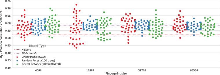
An external validation was employed to confirm that the level of prediction accuracy does not dependent on the complexes deposited in the PDBbind dataset. The Astex Diverse Set was chosen as a source of independently processed, high quality PDB structures. The results of this experiment are shown on Figure 5. The binding affinity predictions made by models trained on PLEC (in terms of R_p) are within a similar range to those observed for the CV experiments, although a higher variance is observed across the FP depths. The Pearson correlation coefficients of the best models are within 0.65–0.7. Again, the linear model was generally as good as neural networks and most of the setups were significantly (up to a 0.2 increase in R_p) better than X-Score (R_p = 0.521) and RF-Score v3 (R_p = 0.586).

Fig. 5.

Prediction results from an independent test set. Correlation coefficients (R_p) for the Astex Diverse Set, depicted with coloured dots. Each dot depicts the result obtained for a particular combination of a model and fingerprint parameters: ligand depth (from 1 to 6), protein depth (from 1 to 6) and fingerprint size (2¹², 2¹⁴, 2¹⁵ and 2¹⁶). Dots are coloured by the model used and separated on the X-axis by the fingerprint size. The red dotted line denotes the X-Score scoring function result, while magenta represents the RF-Score v3 result

3.5 Comparison with state-of-the-art scoring functions and interaction fingerprints

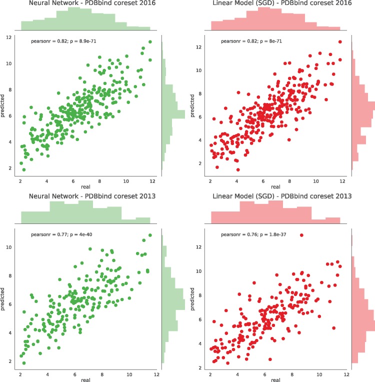
Here, we show a detailed view of the predictive power of the PLEC FP tested on both versions of the ‘core sets’ (v2013 and v2016) and compare it to two recognized IFP representations. As described previously, the PDBbind v2016 ‘general set’ was used as the training set for three different models: linear, random forest and neural network. For the following comparison experiments, a single PLEC FP representation was used with the previously established parameters: an FP size of 65 536, a protein depth of 5, and a ligand depth of 1, which we suggest for general use. Figure 6 depicts the affinity predictions made by the linear model and the neural network. Since our models based on the random forest provided the worst performance of the three methods tested (see Fig. 3 for details), its results are not shown. It is interesting to note that the random forest model benefited the least from increasing the FP size compared to other two models. It seems that the additional data provided by FP sizes larger than 16 384 only marginally influence the random forest learning, leading to a plateau in the prediction results. From the results shown in Figure 3, one can see that the linear model is almost as good at predicting pK_i as the neural network, which highlights the descriptive power of the PLEC FP. The PLEC linear model tested on the v2016 ‘core set’ achieved R_p = 0.817 and standard deviation (SD)  = 1.255 (SD from regression, defined by The comparative assessment of scoring functions (CASF) authors, Li et al., 2014). To the best of our knowledge, this is the best model published to date, in addition to being the least complex one. The PLEC neural network SF did equally well, with R_p = 0.817 and SD = 1.256. Due to the complexity of the neural network (3 dense layers of 200 neurons) compared to the linear model, the latter should be preferred since it is simpler (6 634 401 parameters vs. 65 536, respectively).

Fig. 6.

Detailed view of the prediction accuracy for the PDBbind ‘core sets’. The models were trained on the PLEC representation (FP size 65 536, 5-1 depths). Each dot represents a prediction for a single ligand–receptor complex deposited in the ‘core set’. The left column shows the prediction plots of the neural network, the right column for the linear model. The results for the PDBbind ‘core set’ v2016 are plotted in the upper row and v2013 in the bottom row

Compared to models tested with the CASF-2013 ‘scoring power’ benchmark (Li et al., 2014), the PLEC linear model and the neural network outperform all 20 different SF. In this setup, the PLEC linear model scored R_p = 0.757 and SD = 1.472, while the PLEC neural network achieved R_p = 0.774 and SD = 1.426. This shows significant improvement compared to the best X-Score, which obtained R_p = 0.614 and SD = 1.78.

The PLEC linear model has even outperformed the latest, best ML SF, RF-Score v3, which scored R_p = 0.803 and SD = 1.42 on the ‘core set’ v2016, while providing a much simpler and easier to interpret result.

Finally, we have compared the PLEC FP with two other IFPs. As mentioned in the introduction, there are two main approaches to IFP: (i) explicit definition of the interactions, such as in SILIRID (Chupakhin et al., 2014) and (ii) use of implicit interactions, such as in SPLIF (Da and Kireev, 2014), which employs ECFP environments to define the interactions.

The affinity prediction models were trained and tested using the same procedure as described for the PLEC models. Briefly, the PDBbind v2016 ‘general set’ was used as a training set. The PDBbind ‘core set’ v2016 was used as an independent test set. The SILIRID and SPLIF and PLEC interaction descriptions were the input for linear, random forest and neural network models. Note that explicit FPs such as SILIRID have predefined sizes; thus, there is only one variant for each model.

Direct comparison to these two state-of-the-art IFPs (see Fig. 7) shows the descriptive power of the PLEC FP and its improvement over SPLIF, which uses a similar approach for representing interactions. The SILIRID-based linear model scored R_p = 0.36, while the neural network achieved R_p = 0.52. SPLIF with an FP size of 65 536, performed much better, yielding R_p = 0.78 for both the linear and the neural network models. The SPLIF result is on par with the best performing SF (e.g. RF-Score v3 achieved R_p = 0.797). Models trained using the PLEC FP representations showed another substantial gain in prediction accuracy, obtaining R_p = 0.817 with the neural network and R_p = 0.817 with the linear model.

Fig. 7.

A single R_p value (Pearson correlation coefficient) for each model built on PDBbind v2016 ‘core set’ using the SILIRID, SPLIF and PLEC fingerprints. SILIRID is an explicit interaction fingerprint and has a fixed size; thus, it is presented as a horizontal dotted line. All the models trained using SILIRID are inferior to the others. In addition, the PLEC FP models outperform their SPLIF counterparts

4 Availability and implementation

The PLEC FP has been implemented in the Open Drug Discovery Toolkit (ODDT) (Wójcikowski et al., 2015) and can be used with the RDKit and/or OpenBabel backend. ODDT is available on GitHub [https://github.com/oddt/oddt] on a 3-clause BSD licence. Additionally, SF based on the linear model (PLEC-linear) and the neural network (PLEC-nn) can be accessed via ODDT CLI without any programming knowledge, e.g. to rescore docking results.

5 Conclusions

Herein, we present a novel FP, PLEC and demonstrate its application as an input for binding affinity predictions. The PLEC FP implicitly enumerates protein–ligand contacts, which further allows the predictive models to automatically classify the impact of each contact on the affinity of the compound. The best-performing depths of the PLEC FP are 5 and 1 for the protein and the ligand, respectively, which roughly corresponds to the side chains of residues on the protein side and single atoms on the ligand side. We also demonstrated that the preferable FP size is 65 536, although shorter FPs, combined with more complex models, can achieve comparable performance.

The presented solution performs substantially better than any other method used to represent receptor–ligand complexes in predictive models to date. We also demonstrate the consistent predictive performance of different ML models built using the PLEC FP. This consistency is likely a consequence of the feature power, rather than the model complexity. Our results suggest that the linear model should be preferred since it is simpler and more easily interpretable, although we note that additional performance can be gained in certain cases when using neural networks.

The PLEC FP and SF are freely available as a part of the Open Drug Discovery Toolkit at https://github.com/oddt/oddt. PLEC FP and other functionalities implemented in ODDT can be easily tested via a web browser using MyBinder, see https://github.com/oddt/notebooks.

Funding

This work was supported by the Polish Ministry of Science and Higher Education (POIG.02.03.00-00-003/09-00 and IP2010 037470).

Conflict of Interest: none declared.

References

- Abadi M. et al. (2016) TensorFlow: a system for large-scale machine learning. arXiv: 1603.04467 [cs.DC].
- Axen S.D. et al. (2017) A simple representation of three-dimensional molecular structure. J. Med. Chem., 60, 7393–7409. [DOI] [PMC free article] [PubMed] [Google Scholar]
- Chen B. et al. (2012) Comparison of random forest and Pipeline Pilot Naïve Bayes in prospective QSAR predictions. J. Chem. Inf. Model., 52, 792–803. [DOI] [PubMed] [Google Scholar]
- Chupakhin V. et al. (2013) Predicting ligand binding modes from neural networks trained on protein-ligand interaction fingerprints. J. Chem. Inf. Model., 53, 763–772. [DOI] [PubMed] [Google Scholar]
- Chupakhin V. et al. (2014) Simple ligand-receptor interaction descriptor (SILIRID) for alignment-free binding site comparison. Comput. Struct. Biotechnol. J., 10, 33–37. [DOI] [PMC free article] [PubMed] [Google Scholar]
- Da C., Kireev D. (2014) Structural protein-ligand interaction fingerprints (SPLIF) for structure-based virtual screening: method and benchmark study. J. Chem. Inf. Model., 54, 2555–2561. [DOI] [PMC free article] [PubMed] [Google Scholar]
- Deng Z. et al. (2004) Structural interaction fingerprint (SIFt): a novel method for analyzing three-dimensional protein-ligand binding interactions. J. Med. Chem., 47, 337–344. [DOI] [PubMed] [Google Scholar]
- Gomes J. et al. (2017) Atomic convolutional networks for predicting protein-ligand binding affinity. arXiv: 1703.10603 [cs.LG].
- Huber P.J. (1964) Robust estimation of a location parameter. Ann. Math. Stat., 35, 73–101. [Google Scholar]
- Li H. et al. (2015) Improving AutoDock Vina using random forest: the growing accuracy of binding affinity prediction by the effective exploitation of larger data sets. Mol. Inform., 34, 115–126. [DOI] [PubMed] [Google Scholar]
- Li Y. et al. (2014) Comparative assessment of scoring functions on an updated benchmark: 2. evaluation methods and general results. J. Chem. Inf. Model., 54, 1717–1736. [DOI] [PubMed] [Google Scholar]
- Liu Z. et al. (2017) Forging the basis for developing protein-ligand interaction scoring functions. Acc. Chem. Res., 50, 302–309. [DOI] [PubMed] [Google Scholar]
- Maggiora G. et al. (2014) Molecular similarity in medicinal chemistry. J. Med. Chem., 57, 3186–3204. [DOI] [PubMed] [Google Scholar]
- O’Boyle N.M., Sayle R.A. (2016) Comparing structural fingerprints using a literature-based similarity benchmark. J. Cheminform., 8, 36.. [DOI] [PMC free article] [PubMed] [Google Scholar]
- Pedregosa F. et al. (2011) Scikit-learn: machine learning in Python. J. Mach. Learn. Res., 12, 2825–2830. [Google Scholar]
- Radifar M. et al. (2013) PyPLIF: python-based protein-ligand interaction fingerprinting. Bioinformation, 9, 325–328. [DOI] [PMC free article] [PubMed] [Google Scholar]
- Rogers D., Hahn M. (2010) Extended-connectivity fingerprints. J. Chem. Inf. Model., 50, 742–754. [DOI] [PubMed] [Google Scholar]
- Sato T. et al. (2010) Combining machine learning and pharmacophore-based interaction fingerprint for in silico screening. J. Chem. Inf. Model., 50, 170–185. [DOI] [PubMed] [Google Scholar]
- Vass M. et al. (2016) Molecular interaction fingerprint approaches for GPCR drug discovery. Curr. Opin. Pharmacol., 30, 59–68. [DOI] [PubMed] [Google Scholar]
- Wang R. et al. (2002) Further development and validation of empirical scoring functions for structure-based binding affinity prediction. J. Comput. Aided Mol. Des., 16, 11–26. [DOI] [PubMed] [Google Scholar]
- Weber J. et al. (2015) VAMMPIRE-LORD: a web server for straightforward lead optimization using matched molecular pairs. J. Chem. Inf. Model., 55, 207–213. [DOI] [PubMed] [Google Scholar]
- Witek J. et al. (2014) An application of machine learning methods to structural interaction fingerprints—a case study of kinase inhibitors. Bioorg. Med. Chem. Lett., 24, 580–585. [DOI] [PubMed] [Google Scholar]
- Wójcikowski M. et al. (2015) Open Drug Discovery Toolkit (ODDT): a new open-source player in the drug discovery field. J. Cheminform., 7, 26.. [DOI] [PMC free article] [PubMed] [Google Scholar]
- Wu Z. et al. (2017) MoleculeNet: a benchmark for molecular machine learning. arXiv: 1703.00564 [cs.LG]. [DOI] [PMC free article] [PubMed]
- Yan Y. et al. (2017) Protein-ligand empirical interaction components for virtual screening. J. Chem. Inf. Model., 57, 1793–1806. [DOI] [PubMed] [Google Scholar]
- Zilian D., Sotriffer C.A. (2013) SFCscore(RF): a random forest-based scoring function for improved affinity prediction of protein-ligand complexes. J. Chem. Inf. Model., 53, 1923–1933. [DOI] [PubMed] [Google Scholar]
Associated Data
This section collects any data citations, data availability statements, or supplementary materials included in this article.