Assessment of different methods for shadow detection in high-resolution optical imagery and evaluation of shadow impact on calculation of NDVI, and evapotranspiration

Abstract

Significant efforts have been made recently in the application of high-resolution remote sensing imagery (i.e., sub-meter) captured by unmanned aerial vehicles (UAVs) for precision agricultural applications for high-value crops such as wine grapes. However, at such high resolution, shadows will appear in the optical imagery effectively reducing the reflectance and emission signal received by imaging sensors. To date, research that evaluates procedures to identify the occurrence of shadows in imagery produced by UAVs is limited. In this study, the performance of four different shadow detection methods used in satellite imagery was evaluated for high-resolution UAV imagery collected over a California vineyard during the Grape Remote sensing Atmospheric Profile and Evapotranspiration eXperiment (GRAPEX) field campaigns. The performance of the shadow detection methods was compared and impacts of shadowed areas on the normalized difference vegetation index (NDVI) and estimated evapotranspiration (ET) using the Two-Source Energy Balance (TSEB) model are presented. The results indicated that two of the shadow detection methods, the supervised classification and index-based methods, had better performance than two other methods. Furthermore, assessment of shadowed pixels in the vine canopy led to significant differences in the calculated NDVI and ET in areas affected by shadows in the high-resolution imagery. Shadows are shown to have the greatest impact on modeled soil heat flux, while net radiation and sensible heat flux are less affected. Shadows also have an impact on the modeled Bowen ratio (ratio of sensible to latent heat) which can be used as an indicator of vine stress level.

Introduction

Unmanned aerial vehicles (UAVs) used for remote sensing (RS) purposes have become a rapidly developing technology for acquiring high-resolution imagery of the earth’s surface. The use of UAVs for monitoring agricultural crop conditions has greatly expanded in recent years due to recent advances in high-resolution aerial image processing and sensor technology. These advances have extended the capability to measure crop conditions from a single field to multiple fields in a small time interval. The MIT Technology Review has listed Agricultural UAVs (or drones) as number one in 10 Breakthrough Technologies of 2014 (http://www.technologyreview.com/lists/technologies/2014/). UAVs now offer sub-meter resolution remote sensing relevant to water management through optical and thermal imagery and evapotranspiration estimation advances. This UAV technology is now being applied to high-value crops such as orchards and vineyards to assess individual plant water use or evapotranspiration (ET) and stress (Ortega-Farías et al. 2016; Nieto et al. 2018). This enhanced sensing capability can provide information of plant water use and symptoms for biotic/abiotic stresses at individual plant scale, a capability not achievable with commercial or NASA satellite data. However, as image resolution increases, new challenges emerge such as data transfer and storage, image processing, and detection and characterization of finer scale features such as plant canopy glint, blurriness due to wind, and shadows. Although in some cases shadows might not be a significant issue, they affect surface reflectance and temperature not accounted for in RS energy balance models, which in turn are likely to cause bias in determining plant water use and stress, among other parameters. Therefore, neglecting the shadow impact on monitoring and detecting plant water use and stress and soil moisture status might well result in less reliable assessments for high-value crops.

Shadows appear when elevated objects, such as buildings or trees, occlude and block the direct light (e.g., sun shortwave radiation) produced by a source of illumination. In some cases, information about shadows can provide additional clues about the geometric shape of the elevated object (Lillesand and Kiefer 2000), the position of the source of light (Bethsda 1997), and the height of the object (Sirmacek and Unsalan 2008). In most cases, the appearance of shadows in an image acquired by RS complicates the detection of objects or areas of interest that are located under the shaded area and thus reflect reduced radiance. The appearance of shadows in aerial imagery may also cause loss of valuable information about features, such as shape, height, and color. Consequently, the darkening effect of shadows increases land cover classification error and causes problems for remote sensing studies, such as calculation of vegetation indices and change detection (Zhu and Woodcock 2012). Typical RS vegetation indices and outputs used in agriculture include NDVI, enhanced vegetation index (EVI), LAI (Carlson and Ripley 1997), ET estimates (Nemani and Running 1989), and land cover classification (Trout and Johnson 2007), among others. In addition, sun position changes lead to moving and changing shadow locations. As a result, shadow detection algorithms have received widespread attention, primarily with respect to the impacts of shadows on satellite RS data.

Multiple studies have been conducted to develop methods that detect shadows in images captured by satellites, and several shadow detection methods have been documented. These methods can be categorized into four groups: (a) unsupervised classification or clustering, (b) supervised classification that employ tools such as artificial neural networks (ANNs) or support vector machines (SVMs), (c) index-based methods, and (d) physical-based methods.

• (a)Unsupervised classification/clustering Xia et al. (2009) presented an unsupervised classification/clustering algorithm to detect shadows using the affinity propagation clustering technique in the hue–saturation–intensity (HSI) color space. Shiting and Hong (2013) presented a clustering-based shadow edge detection method using K-means clustering and punishment rules to modify false alarms. Xia’s results revealed that the proposed method has the capability of producing a robust shadow edge mask.
• (b)Supervised classification/object-based methods Kumar et al. (2002) proposed an object-based method to detect shadows using a color space other than RGB. Siala et al. (2004) worked on a supervised classification method to detect moving shadows using support vectors in the color ratio space. Zhu and Woodcock (2012) presented an object-based approach to detect shadows and clouds in Landsat imagery.
• (c)Index-based methods Scanlan et al. (1990) reported a method to detect and remove shadows in images by partitioning the image into pixel blocks, calculating the mean of each block, and comparing it with the image median. Rosin and Ellis (1995) worked on the impact of different thresholds on the detection of shadows in an index-based method. Choi and Bindschadler (2004) presented an algorithm to detect clouds using normalized difference snow index (NDSI) to match plausible cloud shadow pixels based on solar position and Landsat7 images. Qiao et al. (2017) used normalized difference water index (NDWI) and NDVI to separate shadow pixels from both water bodies and vegetation, and then applied a maximum likelihood classifier (MLC) and support vector machines (SVMs) to classify the shadow pixels. Kiran (2016) converted an RGB color image to a grayscale image using the average of the three bands, and then used Otsus method to define a threshold for differentiating between shadow and non-shadow pixels. Finally, a histogram equalization method was applied to improve the contrast of the grayscale image.
• (d)Physical-based methods Sandnes (2011) used the sun position and shadow length to approximately estimate the geolocation of the sensor. Huang and Chen (2009a) presented a physical approach for detecting the shadows in video imagery and showed that the proposed method can effectively identify the shadows in three challenging video sequences. Also, Huang and Chen (2009b) proposed a method for detecting a moving shadow using physical-based features. In this method, the physical-based color features are derived using a bi-illumination reflection model. More information about physical-based models can be found in Sanin et al. (2012).

Concerning the impact of shadows on vegetation indices and water stress, Ranson and Daughtry (1987) and Leblon et al. (1996) concluded that NDVI estimates were highly sensitive to the shaded part of a forest canopy. Leblon et al. (1996) analyzed the mean sunlit and shadow reflectance spectra of shadows cast by a building and by conifers and hardwood trees on grass, bare soil, and asphalt using the visible and near-infrared bands. Their results indicated that reflectance of hardwood shadows was greater than those of conifers and buildings, except for shadow reflectance on bare soil. Moreover, the average NDVI and the atmospherically resistant vegetation index (ARVI) in sunlit areas could be lower or higher than in shaded areas depending on the surface type and shadow type. Hsieh et al. (2016) analyzed the spectral characteristics in the shadow areas and also investigated the NDVI differences between shaded and non-shaded land covers using high-radiometric resolution digital imagery obtained from Leica ADS-40, Intergraph DMC airborne. They found that digital number (DN) values in shaded pixels are much lower than in sunlit pixels and also reported NDVI mean values in shadows and non-shadows from the vegetation category of 0.38 and 0.64, respectively. Poblete et al. (2018) proposed an approach to detect and remove shadow canopy pixels from high-resolution imagery captured by a UAV using a modified scale invariant feature transformation (SIFT) computer version algorithm and K-means++ clustering. Their results indicated that deletion of shadow canopy pixels from a vineyard leads to an improved relationship between the thermal-based Crop Water Stress Index and stem water potential (13% in terms of the coefficient of determination). They also concluded that the impact of shadow canopy pixel removal should be evaluated for ET models working with high-resolution imagery.

While the literature identifies several shadow detection approaches, a few studies have focused on shadow detection for very high-resolution imagery captured by UAVs. Furthermore, limited work is available that demonstrates how shadows might affect the interpretation of the imagery in terms of vegetation indices, biophysical parameters and ET. Therefore, the objectives of this study were to characterize the advantages and disadvantages of a version of each shadow detection model group using high-resolution imagery captured by UAVs over complex canopy locations such as vineyards, and consider the impacts of shaded pixels on NDVI and ET estimations.

Materials and methods

Area of study and UAV sensor descriptions

The high-resolution images for this study were collected by a small UAV over a Pinot Noir vineyard located near Lodi, California (38.29 N 121.12 W), in Sacramento County as part of the GRAPEX project. It is a drip-irrigated system vineyard in which irrigation lines run along the base of the trellis at 30 cm agl with two emitters (4 liters/hour) between each vine. The training system is with “U”-shaped trellises and canes trained upwards. The vine trellises are 3.35 m apart, and the height to first and second cordons is about 1.45 and 1.9 m, respectively (Kustas et al. 2018). The orientation of the vine rows is east–west. In terms of cycle of vine canopy growth in that area, the bud break (grape flowering state) occurs in early May, and the veraison to harvest stage occurs in early or mid-June to late August. Thus, June, July, and August are the months that the canopy may undergo stress. The UAV was supplied and operated by the AggieAir UAV Research Group at the Utah Water Research Laboratory at Utah State University (http://www.aggieair.usu.edu/). Four sets of high-resolution imagery (20 cm or finer) were captured over the vineyard by the UAV in 2014, 2015, and 2016. These UAV flights were synchronized with Landsat satellite overpass dates and times. The data were used to evaluate the various shadow detection methods. The study area is shown in Fig. 1, and information describing the images is summarized in Table 1. Details of the AggieAir aircraft, along with sensor payload, are shown in Fig. 2.

Fig. 1.

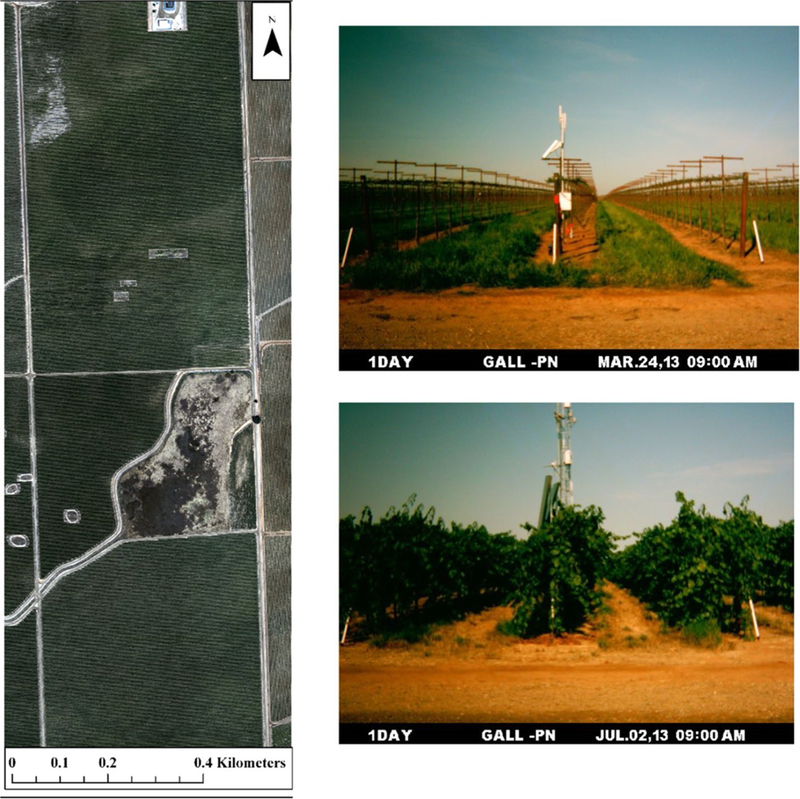
Example of an aerial image of the study area captured by the AggieAir UAV on June 2015 (left), and NASA phenocam photographs for the same site (right, obtained on 24 March 2013 and 02 July 2 2013 during the growing season)

Table 1.

Dates, times, cameras and optical filters used to capture images with the UAV

Date	UAV Flight time (PDT)		UAV eleva- tion (agl) meters	Bands		Cameras and optical filters		Spectral response
	Launch time	Landing time		RGB	NIR	Radio- metric response	MegaPixels
August 9, 2014	11:30 AM	11:50 AM	450	Cannon S95	Cannon S95 modified (Manufacturer NIR block filter removed)	8-bit	10	RGB: typical CMOS NIR: extended CMOS NIR Kodak Wratten 750 nm Long- Pass filter
June 2, 2015	11:21 AM	12:06 PM	450	Lumenera Lt65R Color	Lumenera Lt65R Monochrome	14-bit	9	RGB: typical CMOS NIR: Schneider 820 nm LongPass filter
July 11, 2015	11:26 AM	12:00 PM	450	Lumenera Lt65R Color	Lumenera Lt65R Monochrome	14-bit	12	RGB: typical CMOS NIR: Schneider 820 nm LongPass filter
May 2, 2016	12:53 PM	1:17 PM	450	Lumenera Lt65R Mono	Lumenera Lt65R Mono	14-bit	12	RED: Landsat 8 Red Filter equivalent NIR: Landsat 8 NIR Filter equivalent

Fig. 2.

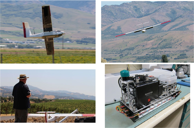
Photos of the AggieAir aircraft and its sensor payload

As described in Table 1, different optical cameras were used each year (2014, 2015, and 2016). Cameras ranged from consumer-grade Canon S95 cameras to industrial type Lumenera monochrome cameras fitted with narrowband filters equivalent to Landsat 8 specifications. The thermal resolution for all four flights was 60 cm and the visible and NIR (VNIR) were 10 cm except for the first one (15 cm).

A photogrammetric point cloud was produced from the multispectral images with a density of 40 (points/m²) for the 15 cm resolution (2014 imagery) and 100 (points/m²) for the 10 cm resolution (2015 and 2016 imagery), after which a digital surface model (DSM) was generated at the same spatial resolution than the original imagery (i.e., 15 cm for 2014 and 10 cm for 2015 and 2016). In addition to UAV point cloud products that describe the surveyed surface, a LiDAR-derived bare soil elevation (digital terrain model DTM) product for the same location, collected by the NASA G-LiHT project, was used Cook et al. (2013). Also, 2014 and 2015 images were captured between veraison and harvest stage, and the 2016 flight was between bloom and veraison stages (Table 2).

Table 2.

Dates, optical, DSM and thermal resolution, point cloud density and phenological stages of the vineyard when the images are captured by the UAV

Dates	Optical and DSM resolu- tion	Thermal resolu- tion	Point cloud density (points/m2)	Phenological stage
9-Aug-14	15 cm	60 cm	37	Near harvest
2-June-15	10 cm	60 cm	118	Near veraison
11-Jul-15	10 cm	60 cm	108	Veraison to harvest
2-May-16	10 cm	60 cm	77	Bloom to veraison

Following the imagery acquisition, a two-step image processing phase occurred, including (1) radiometric calibration and (2) image mosaicking and orthorectification. In the first step, the digital images are converted into a measure of reflectance by estimating the ratio of reference images from pre- and post-flight Labsphere (https://www.labsphere.com/) Lambertian panel readings. For this conversion, a method has been adapted from Neale and Crowther (1994), Miura and Huete (2009), and Crowther (1992) that is based solely on the reference panel readings, which do not require solar zenith angle calculations. This procedure additionally corrected camera vignetting effects that were confounded in the Lambertian panel readings. In the second step, all images were combined into one large mosaic and rectified into a local coordinate system (WGS84 UTM 10N) using the Agisoft Photoscan software AgiSoft (2016), and survey-grade GPS ground measurements. The software produced hundreds of tie-points between overlapping images using photogrammetric principles in conjunction with image GPS log file data and UAV orientation information from the on-board Inertial Measurement Unit (IMU) to refine the estimate of the position and orientation of individual images. The output of this step is an orthorectified reflectance mosaic (Elarab et al. 2015). For thermal imagery processing, only step 2 is applied. The resulting thermal mosaic was brightness temperature in degree Celsius. Moreover, a vicarious calibration for atmospheric correction of microbolometer temperature sensors proposed by Torres-Rua (2017) was applied to the thermal images.

Shadow detection methods

Figure 3 provides a schematic overview of the four different shadow detection methods that were evaluated in this study. For unsupervised k-means classification, the value of k (maximum number of classes) must be determined. When using supervised classification, the signature spectra for each of the categories must be previously identified. The index-based method required that an index be calculated using two or more spectral bands and the identification of a threshold value (digital number or reflectance). Because the shadowed pixels can be visually identified, the threshold value can be modified in a trial-and-error process. Application of the physical-based model involved calculation of the sun position based on the central latitude and longitude of the imagery, together with the local time at the flight area. Since the case study is not a large area (<1.4 km²) and the flight time is less than 20 min, we can assume that the sun position is constant for all pixels.

Fig. 3.

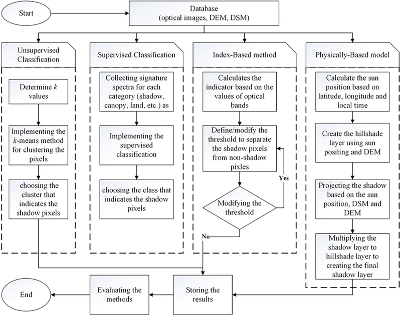
Flowchart illustrating the process of the study for evaluating the shadow detection methods using the very high resolution images captured by UAV

To statistically determine the impact of shadows over NDVI, a standard analysis of variance (ANOVA) analysis was implemented. The ANOVA analysis compared shadowed and non-shadowed pixels over the canopy and was applied to the best of the four shadow detection methods.

To separate the canopy pixels from ground pixels, DTM and DSM products for each image acquisition date are used. If the difference between DSM and DTM was greater than a threshold (e.g., 30 cm), that pixel could be considered as belonging to the canopy vegetation; otherwise, it was assumed to be a pixel of bare ground/inter-row. This threshold filtered the canopy pixels in the images and its selection included a trial-and-error process.

Afterward, based on the filtering procedure and the evaluation of the shadow detection methods, the leaf canopy portions that were shaded or sunlit were extracted. From here, NDVI was calculated and estimated separately for the shaded and sunlit portions of the canopy. For NDVI, the shadowed versus sunlit pixels were compared to each other in terms of histogram analysis and ANOVA. The null hypothesis for the ANOVA test is that the average of the two populations are similar (e.g., the mean values of the shaded and sunlit NDVI pixels were equal). If the null hypothesis was rejected, a further comparison was performed on how the difference in shaded versus sunlit could affect NDVI and ET.

Results and discussion

Unsupervised classification (clustering)

Examples of the results of unsupervised classification (clustering) for shadow detection are illustrated in Fig. 4 for the various flight dates over the study area. Five clusters were considered in applying the clustering method. These were generated based on the k-means method. The unsupervised classification toolbox of the ERDAS Imagine Software was used to execute the k-means algorithm. As shown in Fig. 4, it is evident that most of the pixels assigned to Cluster 1 represent the pixels in shadows. Clusters 2 and 3 were mostly related to the sunlit vegetation canopy, and most of the pixels categorized into Clusters 4 and 5 were bare soil. In addition, some parts of the bare soil in the central part (dark pixels) of the 2015 images were classified as shadowed pixels (Cluster 1), which was not correct. Also, in the May 2016 image, some pixels classified in Cluster 5 (which were mostly bare soil pixels) overlapped with vegetation pixels. Thus, each cluster is a mixture of at least two features (shadow, soil, etc.) as different levels of shade (particularly, the shadow over the canopy in the vine row) can be found in Cluster 2 not in Cluster 1. As shown in Table 1, only the red and NIR bands were used in 2016. This might have affected the performance of classification because it employed less information than was used for the imagery from the 2014 and UAV flights.

Fig. 4.

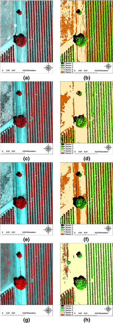
Original UAV false color image subset (left column) and unsupervised classification results (right column) from the vineyard imagery. a, b August 2014, c, d June 2015, e, f July 2015, and g, h May 2016. Black pixels on the right column represent shaded locations

Supervised classification

The supervised classification results were obtained using the supervised classification of the ERDAS Imagine Software. Before running this model, a signature file was collected for each of the different targets (vegetation, shadow, bare soil) using the area of interest layers as the training areas and signature editor. Then each pixel was assigned to these discrete signature classes based on a maximum likelihood method. The results of the supervised classification method for shadow detection in images captured by the UAV in August 2014, June 2015, July 2015, and May 2016 are shown in Fig. 5. From visual inspection, which is the customary approach used to evaluate the performance of different shadow detection methods (Tolt et al. 2011), the performance of this classification for detecting shadows was better than that of the clustering approach, as can be seen by comparing the black pixels in the classified image to the pixels that are obviously in shadows in the false color image. In this method, however, selecting the targets and assigning them to classes was time consuming.

Fig. 5.

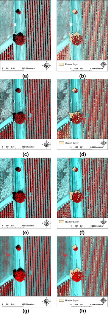
Original UAV false color image subset (left column) and supervised classification results (right column) from the vineyard imagery. a, b August 2014, c, d June 2015, e, f July 2015, and g, h May 2016. Beige pixels on the right column represent shaded locations

Index- or pixel-based methods

A MATLAB program was written for detecting shadowed pixels using the index-based method. In this program, the average of red and NIR bands was considered as a grayscale image. Then, based on a trial-and-error search, a threshold was applied to the grayscale image to separate shadowed from non-shadowed pixels. The results of the index-based method are illustrated in Fig. 6. Again, from visual inspection of these figures, the performance of the index-based approach for detecting shadows is better than that of clustering, and somewhat better than that of the classification method. However, as discussed previously, to identify the shadowed pixels with this method, threshold values must be defined to separate the shadowed area from the original version of the image, which requires a trial-and-error approach and a visual histogram analysis.

Fig. 6.

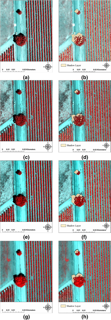
Original UAV false color image subset (left column) and index-based method classification results (right column) from the vineyard imagery. a, b August 2014, c, d June 2015, e, f July 2015, and g, h to May 2016. Beige pixels on the right column represent shaded locations

Physical-based methods

The hillshade toolbox of ArcGIS was executed to project shadows according to the solar position, using the UAV DSM data. The results of this modeling are shown in Fig. 7. These images show some uncertainties within the leaf canopy when projecting the shadows using these tools. Although the ArcGIS hillshade toolbox is independent of the reflectance of each pixel, several factors can affect its accuracy. First, to execute the hillshade toolbox, the solar position (azimuth and elevation) must be defined. Based upon the latitude and longitude of the image, as well as the time that the image was captured by the UAV, the solar position is defined. Obviously, latitude and longitude are not fixed values over the entire image. Moreover, the duration of the flight is around 20 minutes or less. Therefore, the solar position is not consistent relative to all pixels, so the average solar position was used as input. Moreover, the accuracy of the hillshade projection critically depends upon the accuracy of the DSM. Similar to the index-based method, separating the shadowed area from the image required a threshold. Thus, uncertainties for the ArcGIS hillshade method could be attributed to one or more of the following sources: (1) the accuracy of the DSM, (2) the threshold definition, (3) the use of an average value for the time at which the image was captured by the UAV, and (4) the use of an average value for latitude/longitude.

Fig. 7.

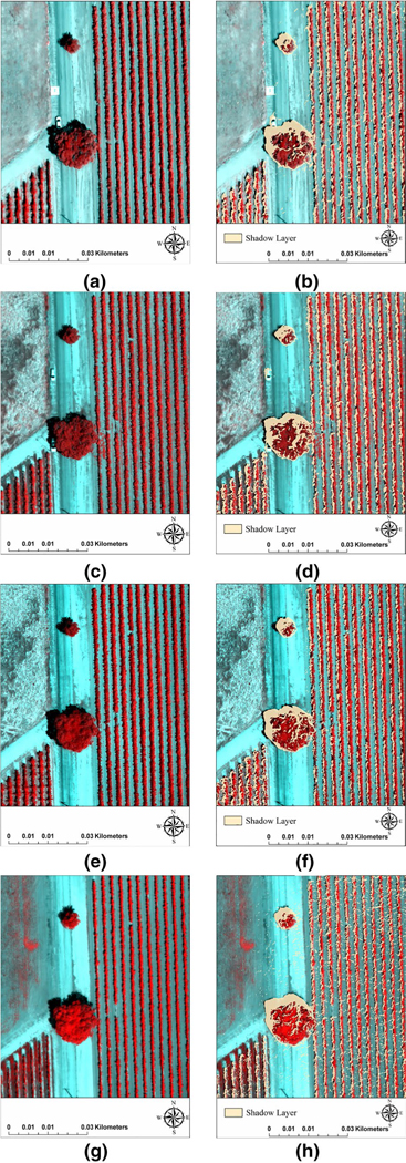
Original UAV false color image subset (left column) and physical-based method classification results (right column) from the vineyard imagery. a, b August 2014, c, d June 2015, e, f July 2015, and g, h May 2016. Beige pixels on the right column represent shaded locations

The Hillshade Toolbox in ArcGIS was executed to project shadows according to solar time and position and DSM. Although the ArcGIS Hillshade Toolbox is independent of pixel reflectance, the main factor that can affect its performance is related to DSM accuracy. Similar to the index-based method, separating the shadowed area required a threshold selection. One advantage of using this method is the ability to generate the shadow layer in the absence of optical imagery. This is illustrated in Fig. 8, wherein the diurnal shadow layer for a small part of the vineyard imagery captured by the UAV in July 2015 is simulated from 7:00 a.m. to 8:00 p.m.

Fig. 8.

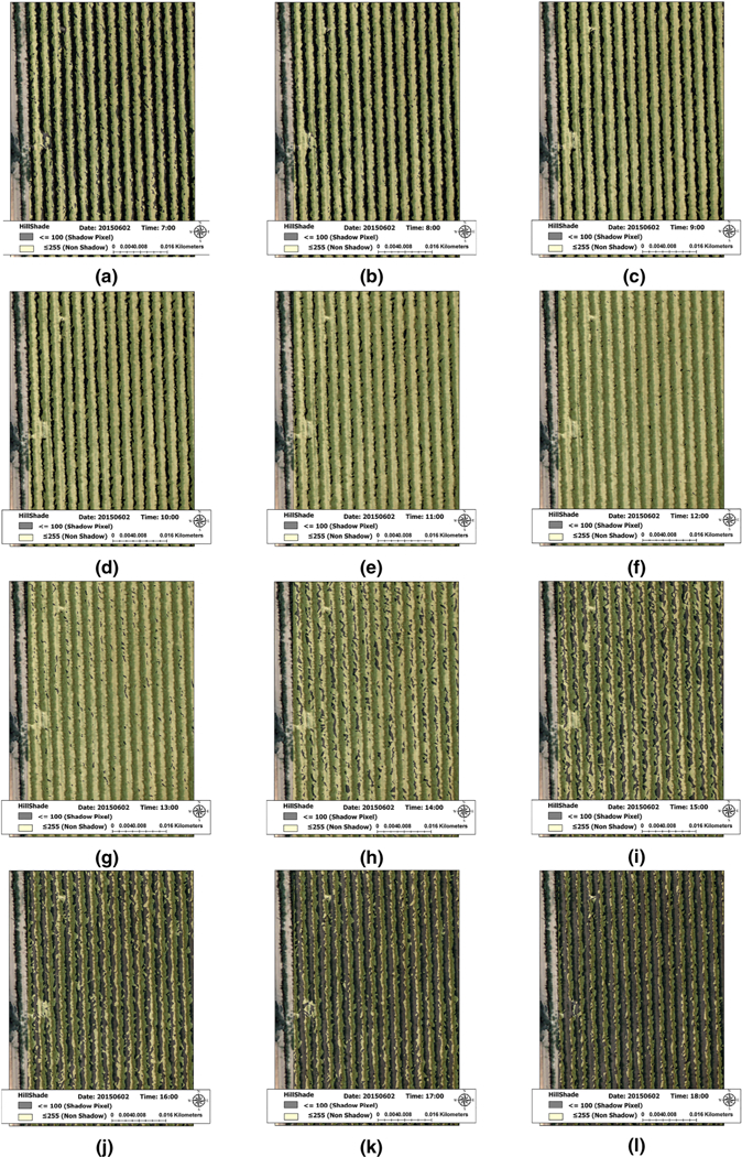
Simulated diurnal shadow pattern shown hourly, from 7:00 a.m. to 8:00 p.m., using the physical-based model and shown on the background image captured by the UAV on July 2015 around 11:45 am PST. shadow layer for 7:00 a.m. (a), 8:00 a.m. (b), 9:00 a.m. (c), 10:00 a.m. (d), 11:00 a.m. (e), 12:00 a.m. (f), 1:00 p.m. (g), 2:00 p.m. (h), 3:00 p.m. (i), 4:00 p.m. (j), 5:00 p.m. (k), and 6:00 p.m. (l). Dark areas indicate shadow locations

Visual assessment of shadow detection model performance

Figure 9 illustrates the shadow detection differences produced by the different classification methods over an area in the approximate center of the GRAPEX vineyard for imagery captured from the various UAV flights. The performance of the unsupervised and supervised classification approaches and the index-based method varies in this region of the image and serves to contrast their performance in detecting shadows.

Fig. 9.

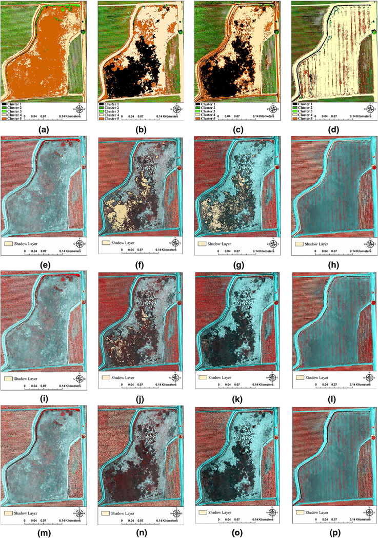
Classification maps of the center portion of the vineyard (original UAV false color image) using unsupervised classification for August of 2014 (a), June of 2015 (b), July of 2015 (c), and May of 2016 (d); using supervised classification for August of 2014 (e), June of 2015 (f), July of 2015 (g), and May of 2016 (h); using the index-based method for August of 2014 (i), June of 2015 (j), July 2015 (k), and May of 2016 (l); using physical-based method for August of 2014 (m), June of 2015 (n), July of 2015 (o), and May of 2016 (p)

From visual inspection of the imagery in Fig. 9, the performance of these four classification methods in the center portion of the vineyard for the flights in August of 2014 (Fig. 9a, e, i, m) and May of 2016 (Fig. 9d, h, l, p) is acceptable. However, for the flights in June of 2015 (Fig. 9b, f, j, n) and in July of 2015 (Fig. 9c, g, k, o), the physical-based classification methods performed much better than the unsupervised, supervised, and index-based classification methods in the flat region (the center area) where the gray and black pixels can be classified into the shadow class. In addition, the performance of the index-based method is superior to that of the supervised classification method in July 2015 (Fig. 9g vs. k). Thus, although in the flat area, the physical-based and index-based methods performed similar to each other and much better than the unsupervised, and supervised methods, within the leaf canopy the physical-based method overestimates shadowed pixels (see Figs. 7, 9m–p).

Statistical assessment of shadow detection method performance

Since shadow detection is a classification task, one approach for evaluating the accuracy of the classification methods is to use the confusion matrix and report the correctness metric [or user accuracy as described in Congalton (1991)] shown in (Eq. 1). To create a confusion matrix, the images on the left column of Fig. 5 were manually separated into two categories: (1) shadowed and (2) non-shadowed areas. Afterward, each class in the manually extracted method was compared to the corresponding class in each of the classification methods. Ultimately, the correctness metric (Eq. 1) was calculated based on the confusion matrix. The results of the confusion matrix, along with the correctness metric, are shown in Table 3. According to the correctness metric, the accuracy of the index-based (~94%) method and the supervised (~92%) method is higher than for the unsupervised (~ 83%) method and the physical-based (~87%) method. These results confirmed the visual assessment performed in the previous subsection.

Table 3.

Assessment accuracy between different methods and manually extracted method for a small part of the study of area

Date of flight	Item	Method	Unsupervised		Supervised		Index based		Physical based
			Method		Method		Method		Method
		Classes	Shadow	Non-shadow	Shadow	Non-shadow	Shadow	Non-shadow	Shadow	Non-shadow
2014, August	Manually extracted	Shadow	27,039	6742	31,292	2489	32,683	1098	29,455	4326
		Non-shadow	20,485	170,695	8433	182,747	5608	185,572	10,598	180,582
		Total	47,524	177,437	39,725	185,236	38,291	186,670	40,053	184,908
	Assessment accuracy (correctness metric)		80.6%		93.4%		96.7%		87.2%
2015, June	Manually extracted	Shadow	19,038	3917	21,038	1917	21,393	1562	20,084	2871
		Non-shadow	2566	199,440	2109	199,897	1192	200,814	2456	199,550
		Total	21,604	203,357	23,147	201,814	22,585	202,376	22,540	202,421
	Assessment accuracy (correctness metric)		82.9%		91.6%		93.2%		87.5%
2015, July	Manually extracted	Shadow	11,845	2416	13,030	1231	13,320	941	12,497	1764
		Non-shadow	3454	207,246	2561	208,139	1459	209,241	2964	207,736
		Total	15,299	209,662	15,591	209,370	14,779	210,182	15,461	209,500
	Assessment accuracy (correctness metric)		83.1%		91.3%		93.4%		87.6%
2016, May	Manually extracted	Shadow	18,301	3459	19,668	2092	20,268	1492	18,796	2964
		Non-shadow	5697	197,504	3294	199,907	2314	200,887	4198	199,003
		Total	23,998	200,963	22,962	201,999	22,582	202,379	22,994	201,967
	Assessment accuracy (correctness metric)		84.1%		90.4%		93.1%		86.4%

$${\text{correctness}}_{\text{metric}}=\frac{\text{TP}}{\text{TP}+\text{FN}},$$ (1)

where TP is the number of shadow pixels identified correctly and FN is the number of shadow pixels categorized into non-shadow class.

To summarize the advantages and disadvantages of the shadow detection methods, the clustering approach requires no pre-knowledge of the shadow pixel features and the operator only needs to specify the number of the clusters, but each cluster contains the information of more than one feature. The performance of the unsupervised classification method is lower than supervised, index-based, and physical-based model, particularly near harvest time (August 2014). However, between bloom and veraison stages of the canopy, the unsupervised classification performance is similar to the physical-based method. The supervised classification method requires pre-knowledge of and sample collection for the desired groups such as vegetation and bare soil and is time consuming and expensive, especially if there are numerous targets in the imagery. Despite the phenological stages, the accuracy of supervised classification is quite high (more than 90%), but with thriving canopy its performance improves from 90% (bloom to veraison in May 2016) to 93% (near harvest in August 2014), which is unlike the behavior of the unsupervised classification. In the index-based method, the desired class or target is more sensitive to the threshold that separates the pixels of the desired class from others. Defining an accurate threshold value requires a trial-and-error process that is time consuming; however, the computational time is generally much less than the unsupervised and supervised classification methods. The accuracy of the index-based method is quite high and even better than the supervised classification method. Like the supervised classification method, the weakest performance of the index-based method occurred when the canopy is not well developed (bloom to veraison in May 2016), whereas from closing to the harvest time, its accuracy increases (96%). The physical-based method requires several inputs, including sun position (azimuth and altitude angles) in the sky, data contained in a DTM, and data from a DSM. The physical-based method is independent of the optical imagery and provides an opportunity to model a diurnal pattern of shadow changes over the study area. However, its performance is completely dependent on the quality and spatial resolution of the DEM and DSM data, which is a significant limitation. Its performance classified between the unsupervised and supervised/index-based method. There are no significant changes in the accuracy of the physical-based method with a thriving canopy; however, the supervised, index-based, and physical-based methods all have higher performance in shadow detection during veraison–harvest (June–August) when the canopy may be under stress versus the bloom–veraison.

Impacts of shadows on NDVI and ET

The results of evaluating NDVI in both the sunlit and shaded areas of the vineyard leaf canopy are presented here. As discussed in Materials and methods, assessing the impact of shadows on NDVI involved extracting two groups of pixels, sunlit and shaded, using two steps. The first step separates the vine canopy pixels from the ground surface and inter-row areas using DTM and DSM data. The second step is the results from the index-based shadow detection method. To test the equality of these two groups, ANOVA was used on the NDVI data from Eq. 2. The results of ANOVA for NDVI are presented in Table 4. The null hypothesis in the ANOVA is that the mean in both groups (sunlit pixels and shaded pixels) is equal. The results of ANOVA for all images are presented in Table 4 (where SS is the sum of squares, df is the degrees of freedom, MS is the mean of squares and F is the f statistic).

Table 4.

ANOVA results for NDVI for the different flights acquired between 2014 and 2016

Flight date	Source of variation	SS	df	MS	F (observed)	P value	F (critical)
August 2014	Groups	0.038	1	0.038	4.63	0.06	3.84
	Error	8.058	970	0.008
	Total	8.086	971
June 2015	Groups	0.328	1	0.32	51.92	0.00	3.84
	Error	6.141	972	0.006
	Total	6.469	973
July 2015	Groups	0.043	1	0.04	8.39	0.00	3.84
	Error	6.36	1222	0.005
	Total	6.40	1223
May 2016	Groups	0.216	1	0.21	20.58	0.00	3.84
	Error	10.26	974	0.010
	Total	10.48	975

$$H_0:{\mu }_1={\mu }_2,$$ (2)

$$H_1:{\mu }_1\ne {\mu }_2,$$ (3)

in which H₀ and H₁ are the null and alternative hypotheses, respectively, and μ₁ and μ₂ are the means of the two groups (in this study, NDVI on the sunlit and shaded leaf canopies).

As shown in Table 4, the F statistic (observed value) is greater than the critical value for F. Therefore, the null hypothesis is rejected for all images. This means that there is a statistically significant difference between the values of NDVI for the shadowed and non-shadowed pixels within the vine canopy. The histograms shown in Fig. 10 further illustrate the difference in the distribution of NDVI values for the UAV flights conducted in 2014, 2015, and 2016.

Fig. 10.

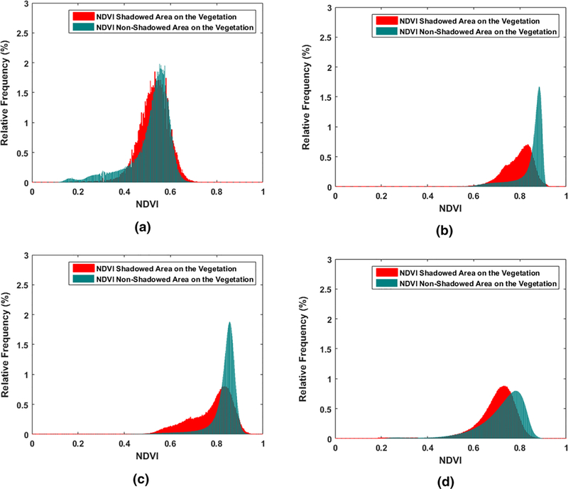
The NDVI histograms for the shadowed and sunlit pixels for the August 2014 imagery (a), the NDVI histograms for the shadowed and sunlit pixels for the June 2015 imagery (b), the NDVI histograms for the shadowed and sunlit pixels for the July 2015 imagery (c), the NDVI histograms for the shadowed and sunlit pixels for the May 2016 imagery (d)

A close examination of the distribution range of the shadowed pixels as presented in Fig. 10 indicates that it is smaller than that of sunlit pixels. In addition, the average values of NDVI in the sunlit pixels are higher than those in the shadowed pixels. This means that ignoring the effect of shadows on NDVI can lead to biased results and conclusions when using this variable. The LAI is a critical input to land surface models for ET estimation that can be calculated based on NDVI. Hence, shadow effects over this biophysical variable will cause error if the models ignore or fail to compensate for the bias on the LAI estimates. For example, in the two-source energy balance (TSEB) model developed by Norman et al. (1995), the radiometric temperature sensed at the satellite is partitioned into canopy temperature (T_c) and soil temperature (T_s) components using the following equation:

$$T_{\text{R}}={\left[f_{\text{c}}(\varphi )T_{\text{c}}^4+\left(1-f_{\text{c}}(\varphi )\right)T_{\text{s}}^4\right]}^{0.25},$$ (4)

where f_c(ϕ) is the fraction of vegetation observed by the thermal sensor with view angle ϕ and can be calculated using the following equation proposed by Campbell and Norman (1998):

$$f_{\text{c}}(\varphi )=1-\exp \frac{-0.5\Omega (\varphi )LAI}{\cos \varphi },$$ (5)

where Ω is a clumping factor and LAI is estimated in this study using an empirical NDVI–LAI relation (Anderson et al. 2004) proposed by Fuentes et al. (2014) for vineyards:

$$LAI=4.4\times NDVI.$$ (6)

Satellite and also UAV imagery provide a single observation of (T_R) per pixel. Therefore, to partition T_R using Eq. 4, there are still two unknown variables, T_c and T_s. One approach to solve the equation is to estimate an initial value for T_c considering plants are transpiring at a potential rate defined by Priestley and Taylor (1972):

$$L{E}_{\text{c}}=\alpha f_{\text{g}}\frac{S}{S+\gamma }R{n}_{\text{c}},$$ (7)

where α is the Priestley–Taylor coefficient (default value is 1.26), f_g is the fraction of vegetation that is green, S is the slope of the saturation vapor pressure curve versus temperature, and γ is the psychrometric constant. Rn_s is the net radiation at the soil surface and Rn_c is the net radiation at the canopy layer estimated based on irradiance, LAI and surface spectra and temperature (Kustas and Norman 1999; Campbell and Norman 1998)

By subtracting LE_c from Rn_c, the sensible heat flux of the canopy (H_c) is achieved. Now, we are able to have an initial estimate of (T_c) using the following equation and solve Eq. 4 with a single unknown variable (T_s):

$$H_{\text{c}}=R{n}_{\text{c}}-L{E}_{\text{c}}=\rho c_p\frac{T_{\text{c}}-T_0}{R_{\text{x}}},$$ (8)

in which ρc_p is the volumetric heat capacity of air, T₀ is the aerodynamic temperature at the canopy interface, and R_x is the bulk canopy resistance to heat transport. In this step, if the soil latent heat flux (LE_s) calculated based on T_s is non-negative, a solution is found. If not, LE_c decreases using an incremental decrease in α, which leads to increasing T_c and decreasing T_s until a non-negative solution for LE_s is found (Norman et al. 1995 and Kustas and Norman 1999). In the case of vineyards, the more sophisticated radiation and wind extinction algorithm in the TSEB model developed by Parry et al. 2017 (this issue) and Nieto et al. 2018) requires several additional inputs, including LAI.

To evaluate the impact of shadows on energy balance components, TSEB was applied considering two scenarios (with and without masking shadows), one in which canopy parameters (LAI, canopy width) are estimated from the original VNIR images, and a second in which the canopy parameters are estimated with the image after masking out the shadows. Moreover, to preserve the assumptions in TSEB related to turbulent transport, TSEB was run by aggregating the UAV imagery to 3.6m. The impact on the magnitude of the energy balance components and their distribution are illustrated in Figures 11, 12, 13, 14 for the UAV image of August 2014. These figures show the spatial absolute differences of fluxes as well as histogram and relative cumulative frequency of fluxes for both scenarios (with and without masking shadows). The histograms show a clear shift in soil heat flux (G) indicating that the peak is moved to the higher values when shadows are involved. Since the NDVI-derived LAIs present smaller values when shaded pixels are involved, LAI yields lower values and, therefore, net radiation reaching the ground (Rn_s) is increased. As G is a ratio of (Rn_s) in TSEB, including the shadows in NDVI–LAI calculation led to an increase of G. For the same scenario, the peak of sensible heat flux (H) and Rn are shifted to smaller values. Increasing G and decreasing Rn account for shadows, and indicate that the available energy (Rn–G) is decreasing. As shown in Fig. 13, H decreased slightly due to slight changes in the soil temperature and canopy temperature values derived from a lower LAI in involving shadows scenario. The latent heat flux (LE) considering the shadows results in a slight shift in the LE distribution to larger values and a greater number of LE values at the centroid of the distribution.

Fig. 11.

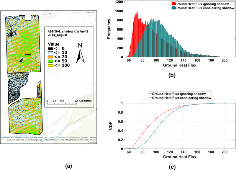
Flight, August 2014; the spatial absolute differences of soil heat flux considering shadows and ignoring shadows (a), histogram of soil heat flux considering/ignoring shadows (b), CDF of soil heat flux considering/ignoring shadows (c)

Fig. 12.

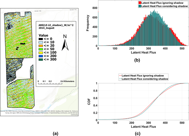
Flight, August 2014; the spatial absolute differences of latent heat flux considering shadows and ignoring shadows (a), histogram of latent heat flux considering/ignoring shadows (b), CDF of latent heat flux considering/ignoring shadows (c)

Fig. 13.

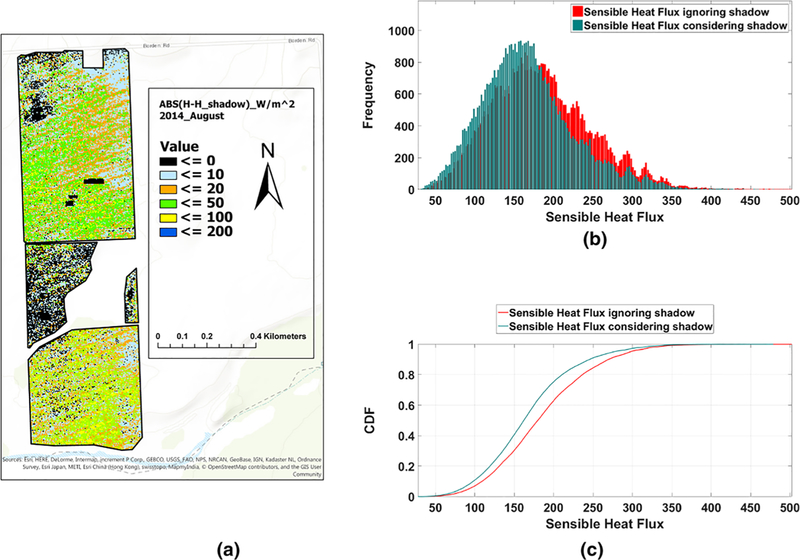
Flight, August 2014; the spatial absolute differences of sensible heat flux considering shadows and ignoring shadows (a), histogram of sensible heat flux considering/ignoring shadows (b), CDF of sensible heat flux considering/ignoring shadows (c)

Fig. 14.

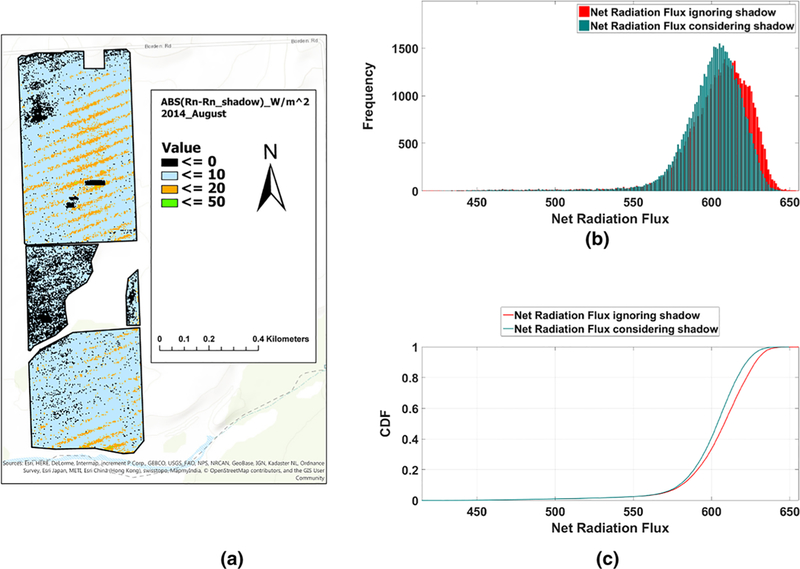
Flight, August 2014; the spatial absolute differences of net radiation flux considering shadows and ignoring shadows (a), histogram of net radiation considering/ignoring shadows (b), CDF of net radiation flux considering/ignoring shadows (c)

An additional evaluation of the shadow impact on crop water stress using Bowen ratio was performed as shown in Figs. 15 and 16. These figures indicate that ignoring shadows led to larger water stress areas, particularly in the southern section of the field. Moreover, the histograms show there are some differences (approximately 6%) in the Bowen ratio calculated by involving versus ignoring the shadows.

Fig. 15.

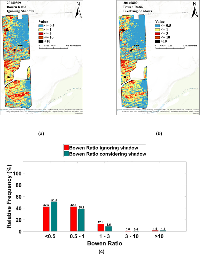
Flight, August 2014; Bowen Ratio ignoring shadows (a), Bowen ratio involving shadows (b), histogram of Bowen ratio ignoring/involving shadows (c)

Fig. 16.

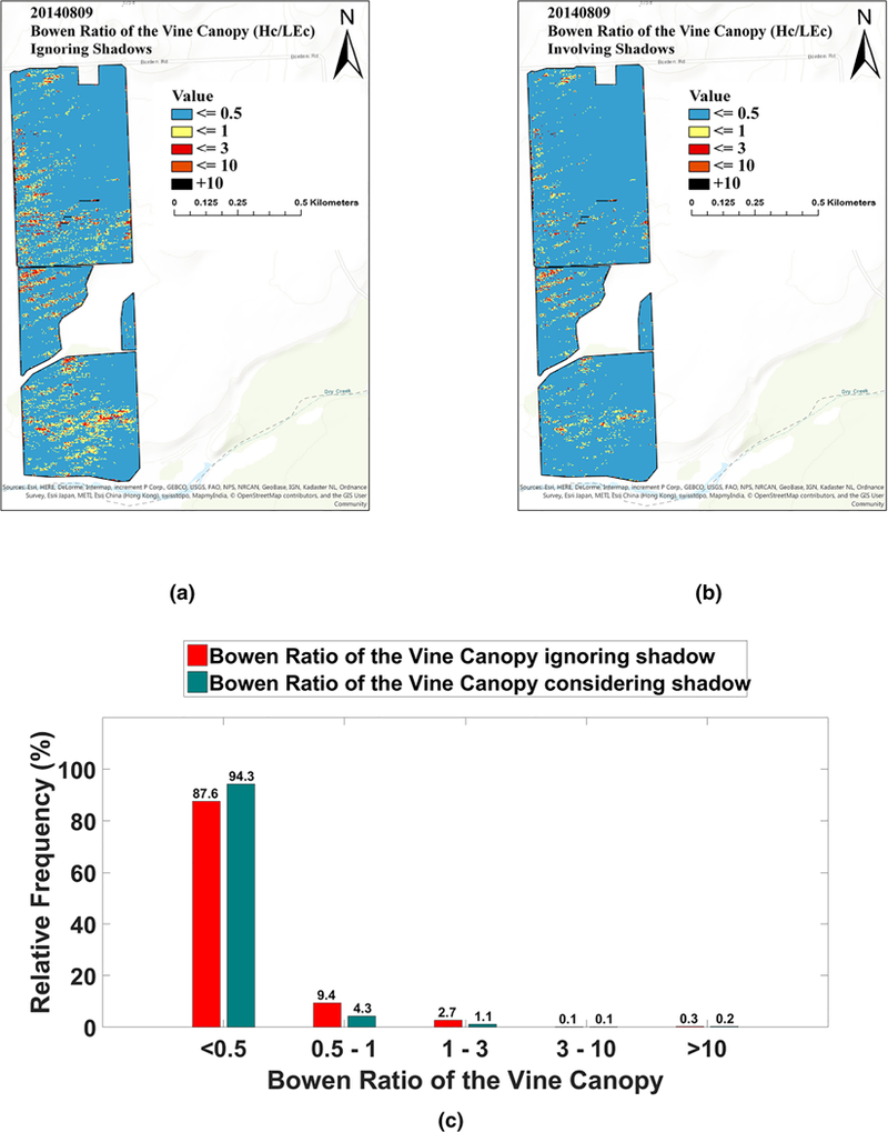
Flight, August 2014; a Bowen ratio of the vine canopy ignoring shadows, b Bowen ratio of the vine canopy involving shadows, c histogram of Bowen ratio of the vine canopy ignoring/involving shadows

The ANOVA test was used to evaluate whether there was a significant difference in the fluxes computed by TSEB when accounting versus ignoring shadows. The results of ANOVA for those fluxes are presented in Tables 5, 6, 7, 8. The ANOVA results indicate that there is a statistically significant difference in ignoring versus accounting for shading for G and, for most of the flights, for Rn. However, in only half the flights does the ANOVA indicate that accounting for shadows makes a difference in the output of H (August 2014 and June 2015 flights) and in only one of the flights for LE (May 2016 flight). Although ANOVA does not indicate a significant difference for LE in 2014 and 2015 flights, it is important to note that ANOVA is used for testing the equality of the means of the distributions and consequently does not evaluate differences in the flux distributions between ignoring and accounting for shadows. For this reason, the spatial differences in the fluxes shown in Figs. 11, 12, 13, 14, 15, 16 indicate the areas of the vineyard where significant discrepancies in fluxes and stress (i.e., Bowen ratio) can exist.

Table 5.

ANOVA results for G flux for the different flights acquired between 2014 and 2016

Parameter	Source of variation	SS	df	MS	F (observed)	P value	F (critical)
August 2014 (G)	Groups	33484.5	1	33484.5	60.73	0	3.84
	Error	550286.6	998	551.4
	Total	583771.1	999
June 2015 (G)	Groups	7064.16	1	7064.16	4.01	0.0456	3.84
	Error	1787208.13	1014	1762.53
	Total	1794272.25	1015
July 2015 (G)	Groups	24355.7	1	24355.7	23.14	0	3.84
	Error	1063052.4	1010	1052.5
	Total	1087408	1011
May 2016 (G)	Groups	13811.9	1	13811.9	13.26	0.0003	3.84
	Error	1035735.6	994	1042
	Total	1049547.5	995

Table 6.

ANOVA results for H flux for the different flights acquired between 2014 and 2016

Parameter	Source of variation	SS	df	MS	F(observed)	P value	F (critical)
August 2014 (H)	Groups	77736.5	1	77736.5	21.82	0	3.84
	Error	3519222.3	988	3562
	Total	3596958.8	989
June 2015 (H)	Groups	58627.9	1	58627.9	3.96	0.0467	3.84
	Error	14544242	984	14781.5
	Total	14,602,869	985
July 2015 (H)	Groups	26698.01	1	26698	1.33	0.2499	3.84
	Error	20,223,718	1004	20143.1
	Total	20,250,416	1005
May 2016 (H)	Groups	2157.86	1	2157.86	0.82	0.3656	3.84
	Error	2,602,439	988	2634.05
	Total	2604596.75	989

Table 7.

ANOVA results for LE flux for the different flights acquired between 2014 and 2016

Parameter	Source of variation	SS	df	MS	F (observed)	P value	F (critical)
August 2014 (LE)	Groups	2280.2	1	2280.2	0.38	0	3.84
	Error	6,000,867	998	6012.89
	Total	6,003,147	999
June 2015 (LE)	Groups	14609.2	1	14609.2	0.59	0.4436	3.84
	Error	24,472,706	984	24870.6
	Total	24,487,316	985
July 2015 (LE)	Groups	4889.28	1	4889.3	0.16	0.6854	3.84
	Error	29,661,146	996	29780.3
	Total	29,666,036	997
May 2016 (LE)	Groups	11763.3	1	11763.3	4.07	0.0439	3.84
	Error	2889741.5	1000	2889.7
	Total	2901504.2	1001

Table 8.

ANOVA results for Rn flux for the different flights acquired between 2014 and 2016

Parameter	Source of variation	SS	df	MS	F (observed)	P value	F (critical)
August 2014 (Rn)	Groups	4022.5	1	4022.48	8.13	0.0044	3.84
	Error	482734.6	976	494.61
	Total	486757.1	977
June 2015 (Rn)	Groups	745.291	1	745.29	0.63	0.4261	3.84
	Error	1140210.55	970	1175.47
	Total	1140955.5	971
July 2015 (Rn)	Groups	4884.997	1	4885	4.06	0.0441	3.84
	Error	1223456.25	1018	1201.82
	Total	1228341.25	1019
May 2016 (Rn)	Groups	1407.9	1	1407.9	3.99	0.0462	3.84
	Error	344,778	976	353.26
	Total	346186.5	977

Conclusions

Shadows are an inherent component of high-resolution RS imagery. If ignored, they can cause bias in products derived from RS data that are intended for monitoring plant and soil conditions. In this study, four different shadow detection methods developed for satellite imagery were applied to very high resolution images captured by a UAV at various times over a GRAPEX vineyard and evaluated for accuracy. These methods were (a) unsupervised classification or clustering, (b) supervised classification, (c) index-based methods, and (d) physical-based methods. The results from visual and statistical assessments indicated that the accuracy of the supervised classification method and the index-based method were generally comparable to one another, and superior to the other two. In terms of phenological stage, the performance of the supervised and index-based methods increases with growing canopy (from bloom stage to harvest stage, when the canopy may be under stress) whereas the accuracy of the unsupervised classification decreases during late growing stage. However, the performance of the physical-based model was not sensitive to the growth stages of the grapevine canopy. Furthermore, an ANOVA assessment between sunlit or shaded canopy indicates statistical differences between the two groups for NDVI. Finally, the impacts of shadows on ET estimation and other fluxes using energy balance models and high-resolution RS data are examined. According to the TSEB model outputs, G increased, while Rn, H, and available energy (Rn–G) decreased in conditions involving shadows. However, in most cases the overall effect on LE was minimal, although differences were significant in certain areas in the vineyard. This implies that high-resolution models of ET and biophysical parameters should consider the impact of shadowed areas that could cause significant bias in modeled ET.

The analyses presented, together with the emerging ability to employ UAV-based remote sensing technologies to acquire high-resolution, scientific-grade spectral data in three dimensions (high-resolution DTM and DSM data, and point cloud data), also point to the possibility of successfully applying high-resolution energy balance modeling techniques to acquire plant-scale estimates of ET and plant stress. Such information could be potentially exploited by growers to manage irrigation deliveries in differential patterns within individual fields while, at the same time, conserving water and reducing management costs. Additional research is required to prove this capability has utility and economic return for high-value crops, such as wine grapes. Future steps based on this work involve the diurnal modeling of shadows for quantification of their impact on energy balance model results, as well as incorporation of shadow conditions into energy balance algorithms.

References

- AgiSoft LLC (2016) and Russia St Petersburg. Agisoft photoscan. Professional Edition
- Anderson MC, Neale CMU, Li F, Norman JM, Kustas WP, Jayanthi H, Chavez J (2004) Upscaling ground observations of vegetation water content, canopy height, and leaf area index during SMEX02 using aircraft and Landsat imagery. Rem Sens Environ 92:447–464 [Google Scholar]
- Bethsda MD (1997) Manual of photographic interpretation. 2nd edition, American Society Photogrammetry and remote sensing (ASPRS) [Google Scholar]
- Congalton RG (1991) A review of assessing the accuracy of classifications of remotely sensed data. Rem Sens Environ 37(1):35–46 [Google Scholar]
- Campbell GS, Norman JM (1998) An introduction to environmental biophysics. Springer, New York [Google Scholar]
- Carlson TN, Ripley DA (1997) On the relation between NDVI, fractional vegetation cover, and leaf area index. Rem Sens Environ 62(3):241–252 [Google Scholar]
- Choi H, Bindschadler R (2004) Cloud detection in Landsat imagery of ice sheets using shadow matching technique and automatic normalized difference snow index threshold value decision. Rem Sens Environ 91(2):237–242 [Google Scholar]
- Crowther BG (1992) Radiometric calibration of multispectral video imagery. Doctoral dissertation. State University. Department of biological and Irrigation Engineering, Utah [Google Scholar]
- Elarab M, Ticlavilca AM, Torres-Rua AF, Maslova I, McKee M (2015) Estimating chlorophyll with thermal and broadband multispectral high resolution imagery from an unmanned aerial system using relevance vector machines for precision agriculture. Int J Appl Earth Obs Geoinform 43:32–42 [Google Scholar]
- Fuentes S, Poblete-Echeverra C, Ortega-Farias S, Tyerman S, De Bei R (2014) Automated estimation of leaf area index from grapevine canopies using cover photography video and computational analysis methods. Aust J Grape Wine Res 20(3):465–473 [Google Scholar]
- Gonzalez RC, Woods RE, Eddins SL (2004) Digital image processing using MATLAB, Prentice Hall [Google Scholar]
- Hsieh YT, Wu ST, Chen CT, Chen JC (2016) Analyzing spectral characteristics of shadow area from ADS-40 high radiometric resolution aerial images. Int Arch Photogram, Rem Sens Spatial Inf Sci XLI–B7:223–227 http://www.aggieair.usu.edu/https://www.labsphere.com/ http://www.technologyreview.com/lists/technologies/2014/ [Google Scholar]
- Huang J, Chen C (2009a) A physical approach to moving cast shadow detection. IEEE international conference on acoustics, speech and signal processing, 769–772 [Google Scholar]
- Huang J, Chen C (2009b) Moving cast shadow detection using physics-based features. IEEE conference on computer vision and pattern recognition, 2310–2317 [Google Scholar]
- Kiran TS (2016) A framework in shadow detection and compensation of images. DJ J Adv Electron Commun Eng 2(3):1–9 [Google Scholar]
- Kumar P, Sengupta K, Lee A (2002) A comparative study of different color spaces for foreground and shadow detection for traffic monitoring system. In: The IEEE 5th International Conference on Intelligent Transportation Systems, 100–105 [Google Scholar]
- Kustas WP, Norman JM (1999) Evaluation of soil and vegetation heat flux predictions using a simple two-source model with radiometric temperatures for partial canopy cover. Agric For Meteorol 94(1):13–29. 10.1016/S0168-1923(99)00005-2 [DOI] [Google Scholar]
- Kustas WP, Anderson MC, Alfieri JG, Knipper K, Torres-Rua A, Parry CK, Hieto H, Agam N, White A, Gao F, McKee L, Prueger JH, Hipps LE, Los S, Alsina M, Sanchez L, Sams B, Dokoozlian N, McKee M, Jones S, Yang Y, Wilson TG, Lei F, McElrone A, Heitman JL, Howard AM, Post K, Melton F, Hain C (2018) The Grape Remote sensing Atmospheric Profile and Evapotranspiration experiment (GRAPEX). Bull Am Meteorol Soc. 10.1175/BAMS-D-16-0244.1 [DOI] [PMC free article] [PubMed] [Google Scholar]
- Leblon B, Gallant L, Charland SD (1996a) Shadowing effects on SPOT-HRV and high spectral resolution reflectance in Christmas tree plantation. Int J Rem Sens 17(2):277–289 [Google Scholar]
- Leblon B, Gallant L, Grandberg H (1996b) Effects of shadowing types on ground-measured visible and near-infrared shadow reflectance. Rem Sens Environ 58(3):322–328 [Google Scholar]
- Lillesand TM, Kiefer RW (2000) Remote sensing and image interpretation, 4th edn New York, Wiley [Google Scholar]
- Miura T, Huete AR (2009) Performance of three reflectance calibration methods for airborne hyperspectral spectrometer data. Sensors 9(2):794–813 [DOI] [PMC free article] [PubMed] [Google Scholar]
- Oy MosaicMill (2009) EnsoMOSAIC image processing users guide. Version 7.3. Mosaic Mill Ltd; Finland [Google Scholar]
- Cook BD, Corp LW, Nelson RF, Middleton EM, Morton DC, McCorkel JT, Masek JG, Ranson KJ, Ly V, Montesano PM (2013) NASA Goddard’s lidar, hyperspectral and thermal (G-LiHT) airborne imager. Rem Sens 5:4045–4066. 10.3390/rs5084045 [DOI] [Google Scholar]
- Neale CM, Crowther BG (1994) An airborne multispectral video/radiometer remote sensing system: development and calibration. Rem Sens Environ 49(3):187–194 [Google Scholar]
- Nemani RR, Running SW (1989) Estimation of regional surface resistance to evapotranspiration from NDVI and thermal IR AVHRR data. J Appl Meteorol 28(4):276–284 [Google Scholar]
- Nieto H, Kustas W, Torres-Rua A, Alfieri J, Gao F, Anderson M, White WA, Song L, Mar Alsina M, Prueger J, McKee M, Elarab M, McKee L (2018) Evaluation of TSEB turbulent fluxes using different methods for the retrieval of soil and canopy component temperatures from UAV thermal and multispectral imagery. Irrigation Sci. 10.1007/s00271-018-0585-9 [DOI] [PMC free article] [PubMed] [Google Scholar]
- Norman JM, Kustas WP, Humes KS (1995) Source approach for estimating soil and vegetation energy fluxes in observations of directional radiometric surface temperature. Agric For Meteorol 77:263–293 [Google Scholar]
- Ortega-Farias S, Ortega-Salazar S, Poblete T, Kilic A, Allen R, Poblete-Echeverra C, Ahumada-Orellana L, Zuiga M, Seplveda D (2016) Estimation of energy balance components over a drip-irrigated olive orchard using thermal and multispectral cameras placed on a helicopter-based unmanned aerial vehicle (uav). Rem Sens 8(8) [Google Scholar]
- Parry C, Nieto H, Guillevic P, Agam N, Kustas B, Alfieri J, McKee L, McElrone AJ. An intercomparison of radiation partitioning models in vineyard row structured canopies. Irrigation Sci (In press) [Google Scholar]
- Poblete T, Ortega-Farias S, Ryu D (2018) Automatic coregistration algorithm to remove canopy shaded pixels in UAV-borne thermal images to improve the estimation of crop water stress index of a drip-irrigated cabernet sauvignon vineyard. Sensors 18(2):397. [DOI] [PMC free article] [PubMed] [Google Scholar]
- Priestley CHB, Taylor RJ (1972) On the assessment of surface heat flux and evaporation using large-scale parameters. Mon Weather Rev 100:81–92 [Google Scholar]
- Qiao X, Yuan D, Li H (2017) Urban shadow detection and classification using hyperspectral image. J Indian Soc Rem Sens. 10.1007/s12524-016-0649-3 [DOI] [Google Scholar]
- Ranson KJ, Daughtry CST (1987) Scene shadow effects on multispectral response. IEEE Trans Geosci Rem Sens 25(4):502–509 [Google Scholar]
- Rosin PL, Ellis T (1995) Image difference threshold strategies and shadow detection. Br Conf Mach Vision 1:347–356 [Google Scholar]
- Ross J (1981) The radiation regime and architecture of plants In: Lieth H (ed) Tasks for Vegetation Sciences 3 Dr. W. Junk, The Hague, Netherlands [Google Scholar]
- Sandnes FE (2011) Determining the geographical location of image scenes based object shadow lengths. J Signal Process Syst 65(1):35–47 [Google Scholar]
- Sanin A, Sanderson C, Lovell B (2012) Shadow detection: a survey and comparative evaluation of recent methods. Pattern Recognit 45(4):1684–1689 [Google Scholar]
- Scanlan JM, Chabries DM, Christiansen R (1990) A shadow detection and removal algorithm for 2-d images.In: Proceeding IEEE International Conference on Acoustics, Speech, and Signal Processing (ICASSP), pp 2057–2060 [Google Scholar]
- Shiting W, Hong Z (2013) Clustering-based shadow edge detection in a single color image. International Conference on Mechatronic Sciences, Electric Engineering and Computer (MEC), pp 1038–1041 [Google Scholar]
- Siala K, Chakchouk M, Besbes O, Chaieb F (2004) Moving shadow detection with support vector domain description in the color ratios space. In: Proceedings of the 17th IEEE International Conference on Pattern Recognition, pp 384–387 [Google Scholar]
- Sirmacek B, Unsalan C (2008) Building detection from aerial images using invariant color features and shadow information.” Proceedings of the 23rd International Symposium on Computer and Information Sciences (ISCIS 2008), Istanbul, Turkey, October 27–29, pp 1–5 [Google Scholar]
- Tolt G, Shimoni M, Ahlberg J, (2011) A shadow detection method for remote sensing images using VHR hyperspectral and LIDAR data. In: Proceedings of Geoscience and Remote Sensing Symposium, IGARSS, Vancouver Canada, pp 4423–4426 [Google Scholar]
- Torres-Rua A (2017) Vicarious calibration of sUAS microbolometer temperature imagery for estimation of radiometric land surface temperature. Sensors 17:1499. [DOI] [PMC free article] [PubMed] [Google Scholar]
- Trout TJ, Johnson LF (2007) Estimating crop water use from remotely sensed NDVI, crop models, and reference ET. USCID Fourth International Conference on Irrigation and Drainage, Sacramento, California, pp 275–285 [Google Scholar]
- Xia H, Chen X, Guo PA (2009) Shadow detection method for remote sensing images using affinity propagation algorithm. In: Proceedings of the IEEE International Conference on Systems, Man and Cybernetics, San Antonio, TX, USA, pp 5–8 [Google Scholar]
- Zhu Z, Woodcock CE (2012) Object-based cloud and cloud shadow detection in Landsat imagery. Rem Sens Environ 118(15):83–94 [Google Scholar]