Healing the Poor: The Influence of Patient Socioeconomic Status on Physician Supply Responses

Abstract

A longstanding literature explores how altruism affects the way physicians respond to incentives and provide care. We analyze how patient socioeconomic status mediates these responses. We show theoretically that patient socioeconomic status systematically influences the way physicians respond to reimbursement changes, and we identify the channels through which these effects operate. We use two Medicare reimbursement changes to investigate these insights empirically. We confirm that a given physician facing an increase in reimbursement boosts utilization by more when treating richer patients. We show that average supply price elasticities vary from 0.02 to 0.18 for a given physician, depending on the patient’s socioeconomic status. Finally, we show that the Medicare reforms we study led to overall reimbursement increases that raised healthcare utilization by 10% more for high-income patients compared to their low-income peers. JEL: I11, I12, I18

1. Introduction

Economists have long emphasized the peculiarities of healthcare markets, compared to other markets for goods and services. Since at least Kenneth Arrow’s pioneering paper on the subject, economists have recognized two features in particular: the altruism of healthcare providers towards their patients and the reliance of patients on their physicians for information and guidance (Arrow 1963).

Altruism encourages physicians to faithfully represent their patients’ interests. An altruistic physician will tend to economize on the use of scarce inputs and attempt to improve the well-being of her patients. On the other hand, the informational advantage of physicians creates a classic agency problem that physicians might exploit to pursue their own interests at the expense of their patients’ (for example, Dranove and White 1987; Blomqvist 2002; Emanuel and Emanuel 1992; Mooney and Ryan 1993; Zweifel, Breyer, and Kifmann 1997). These countervailing incentives produce conflicting implications for pricing. Self-interested physicians will respond to higher prices by performing more procedures. Altruistic physicians, on the other hand, will protect their patients from higher prices by performing fewer procedures. Prior literature has investigated these complex implications of physician altruism on a variety of outcomes, including physician labor supply, patient health, patient treatment plans, responses to reimbursement changes, optimal insurance design, and quality of care (Chone and Ma 2011; Clemens and Gottlieb 2014; Dickstein 2016; Dranove 1988; Ellis and McGuire 1990; Ellis and McGuire 1986; Godager and Wiesen 2013; Jack 2005; Jacobson et al. 2017; Liu and Ma 2013; McGuire 2000; Rochaix 1989; Glied and Zivin 2002).

Less attention has been paid to the influence of patient socioeconomic status on physician decision making. Intuitively, if physicians care about patient utility, then factors that affect marginal utility– such as patient wealth and income– might systematically alter how a physician behaves, even for otherwise clinically similar patients. Figure 1 offers some suggestive evidence of what this might mean empirically.

Figure 1.

Variation in Price, Utilization, and Income

Notes: Data from the Federal Register and MCBS. Plot (a) shows the median RVUs per physician-patient over time for patient income below (“low income”) and above (“high income”) the median income. Plot (b) shows the median price index for physicians. The price index is calculated as the 1993-utilization weighted average of prices across all services that a physician performs during the time period.

The figure reports a weighted price index over time for Medicare, alongside an index of utilization by high-income and low-income patients. The price index measures the average change in reimbursements for a fixed basket of procedures that are weighted by the intensity required to perform them. In the wake of rapid acceleration in prices, the utilization of high-income patients appeared to rise more rapidly than that of their low-income counterparts.

In this paper, we investigate theoretically and empirically how patient socioeconomic status influences altruistic physicians facing reimbursement changes. We rely on well-established models of physician behavior to explore how patient socioeconomic status influences physicians when patients face positive cost-sharing. We demonstrate theoretically that there are two components to the effect of socioeconomic status. First, when utilization is held fixed across all patients, physicians’ supply response to higher reimbursements will be larger (i.e., more positive) for richer patients. Richer patients face lower marginal disutility of price increases because of their higher incomes. Thus, on the margin, it is less costly for altruistic physicians to “harvest” higher utilization from these patients. Second, however, differences in utilization across richer and poorer patients always give rise to a countervailing “utilization effect” that we elucidate theoretically. Thus, economic theory predicts that the same physician might respond differently to a price change when treating a richer patient, even holding clinical considerations fixed. The direction of the effect becomes an empirical question of interest.

Empirically, we estimate the effect of patient socioeconomic status on physician supply responses by using two exogenous policy shocks to Medicare payments: the 1997 consolidation of geographic payment regions and the 1999 change in estimation of practice expenses. Our results indicate that a given physician’s supply response is stronger when she treats richer patients. Moreover, the variation in price elasticities matters quantitatively. Within physicians, average price elasticities vary from 0.02 to as high as 0.18, when treating patients in the bottom or top socioeconomic status deciles, respectively. Finally, we estimate that our two exogenous policy shocks increased utilization among high-income patients by 10% more than among low-income patients. This effect accounts for about 53% of the divergence across income groups that we see in Figure 1.

The rest of the paper is organized as follows. In Section 2, we investigate the theoretical relationship between patient socioeconomic status and physician supply responses. In Section 3, we discuss the empirical approach for estimating the effects of socioeconomic status on supply responses. In Section 4, we present the empirical results, and Section 5 concludes.

2. Theoretical Framework

We study how variation in patient socioeconomic status influences the way altruistic physicians respond to price. We rely on a simple and stylized model of altruistic decision making that dates back to Becker (1957). The model has been used by many health economists before us to study physician behavior (cf, Clemens and Gottlieb 2014; Ellis and McGuire 1986; Ellis and McGuire 1990; McGuire 2000; McGuire and Pauly 1991; Dickstein 2016).

Consider the treatment of a particular patient by a particular physician.¹ The physician produces health in the patient according to the strictly concave function $F\left(X\right)$, where X is the level of medical care used. We focus on the case where the patient is exposed to some degree of cost-sharing for care because we are interested in how physicians respond when price changes directly impact patient utility. The patient pays $\sigma \left(X;P\right)$ for X amount of medical care, where P is the price for medical care received by the physician, and $\sigma$ is the cost-sharing function that defines the patient’s out-of-pocket cost. Denoting partial derivatives with subscripts, we assume that ${\sigma }_P>0, {\sigma }_X>0, and {\sigma }_{XP}>0$. In addition, we also assume ${\sigma }_{XX}=0$, which rules out nonlinear cost-sharing arrangements. Coinsurance that asks patients to pay a fixed percentage of cost would satisfy all these assumptions. Finally, define the patient’s burden of all other medical care spending as $\pi$; this includes health insurance premiums and out-of-pocket spending on care given by providers other than this particular physician. Assume the representative patient derives strictly concave utility from consumption according to $u\left(I+vF\left(X\right)-\sigma \left(X;P\right)-\pi \right)$. I is income, $v$ is the value of health, and both are measured in units of the same numeraire consumption good.

All medical decisions are made by the physician. This is a stylized assumption that helps focus on the incentives of the physician and motivate our empirical analysis of physician price-responses. The physician cares about her own utility and that of the patient, according to:

$${\max }_X\left(1-\alpha \right)z\left(PX-c\left(X\right)\right)+\alpha u\left(I+vF\left(X\right)-\pi -\sigma \left(X;P\right)\right).$$ (1)

The function $c(\cdot )$ is the physician’s strictly convex cost of providing medical care, and the function $z(\cdot )$ is her weakly concave utility from her own income. The degree of altruism towards the patient is $\alpha$. The first-order condition for medical care utilization can be written as:

$$\alpha u^{\prime }*\left(vF\prime -{\sigma }_X\right)+\left(1-\alpha \right)z^{\prime }*\left(P-c\prime \right)=0$$ (2)

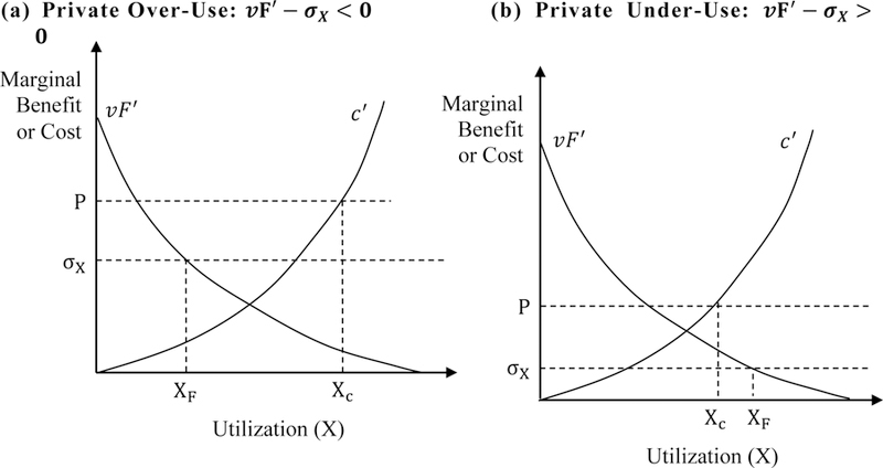
Notice that either $vF\prime -{\sigma }_X<0$ or $P-c\prime <0$.² Therefore, medical care is strictly costly on the margin to either the consumer or the physician, respectively, but never both. Figure 2 depicts the conditions that determine which case prevails. When $vF\prime$ intersects ${\sigma }_X$ before $c\prime$ intersects P, we end up with the case $vF\prime -{\sigma }_X<0$, where care is costly to the consumer on the margin. This corresponds to the left-hand panel of the figure (plot a), where $X_F<X_C$. Conversely, the opposite case obtains when $X_F>X_C$ (plot b).

Figure 2.

Determinants of Optimal Utilization

From the patient’s perspective, $vF\prime -{\sigma }_X<0$ implies “private under-use” of medical care in the sense that more utilization at the equilibrium point would increase her utility. Private under-use is possible in this setting because patients do not directly decide on medical care. Physicians make these decisions, and they will fail to choose the patient’s privately optimal utilization level unless they are perfectly altruistic. For notational convenience, we refer to $vF\prime -{\sigma }_X<0$ as the case of “private over-use” and to $vF\prime -{\sigma }_X>0$ as the case of “private under-use.” For clarity, these cases do not represent social under-use or over-use, but rather over-use and under-use from the patient’s private perspective. All else equal, private over-use is more likely when: marginal value product diminishes more quickly, marginal cost of medical care diminishes more slowly, patient out-of-pocket prices are higher, or physician reimbursements are lower.

2.1. Effect of price and income on utilization

Higher prices can either increase or decrease utilization depending on four distinct and potentially offsetting forces that we will characterize. Differentiating Equation (2) with respect to price results in:

$$\frac{\partial X}{\partial P}=\frac{\left(-\alpha u^{\prime }{\sigma }_{XP}-\alpha u^{″}\left(v{F}^{\prime }-{\sigma }_X\right)\left({\sigma }_P\right)+\left(1-\alpha \right)z^{\prime }+\left(1-\alpha \right)z^{″}\left(P-c^{\prime }\right)X\right)}{\left(-D\right)}.$$ (3)

The denominator is positive, because the second-order condition implies $D\equiv \alpha u^{″}{\left(v{F}^{\prime }-{\sigma }_X\right)}^2+\alpha u^{\prime }\left(v{F}^{″}\right)+\left(1-\alpha \right)z^{″}{\left(P-c^{\prime }\right)}^2+\left(1-\alpha \right)z^{\prime }\left(-c^{″}\right)<0$ omparative static expression depends on the interplay among four distinct and countervailing forces.

1. “Profitability effect” leads to higher output: Higher prices raise the physician’s marginal financial return to providing care, because $\left(1-\alpha \right)z^{\prime }>0$_.

2. “Substitution effect” leads to lower output: Higher prices induce a substitution effect that makes medical care more expensive for the patient, all else equal; an altruistic physician cuts output in response, because $\left(-\alpha u^{\prime }{\sigma }_{XP}\right)<0$_.

3. “Patient income effect” leads to lower or higher output: Higher prices make the patient poorer, and this encourages the physician to transfer additional “net consumption” to the patient. In the private over-use case, the physician cuts medical care utilization to accomplish this, because $\left(-\alpha u^{″}\left(v{F}^{\prime }-{\sigma }_X\right)\left({\sigma }_P\right)\right)<0$. In the private under-use case, she raises medical care utilization to achieve the same end.

4. “Physician income effect” leads to lower or higher output: Higher prices make the physician richer, and this encourages her to transfer additional “net consumption” to the patient. In the private over-use case, the physician (weakly) cuts medical care utilization to accomplish this, because $\left(1-\alpha \right)z^{″}\left(P-c\prime \right)X\le 0$_. In the private under-use case, the opposite occurs. Note this effect disappears when the physician’s objective function is quasi-linear in her own income, a case we explore in more detail below.

In principle, price increases can either increase or decrease utilization. When $\frac{\partial X}{\partial P}>0$, we can think of supply as “physician-driven” in the sense that physician preferences for profit dominate in the sign of the supply response. Conversely, when $\frac{\partial X}{\partial P}<0$, we can think of it as “patient-driven,” since patients’ downward-sloping demand for care dominates in the sign of this response.

The effect of patient income on prices is analogous to the “patient income effects” described above. In the case of private over-use, physicians will cut utilization when patients are poorer, in an effort to make them better off. However, with private under-use, physicians will actually raise utilization for poorer patients to accomplish the same objective. These results become evident in another comparative static expression that follows from the first-order condition:

$$\frac{\partial X}{\partial I}=\frac{\left[\alpha u^{″}\left(v{F}^{\prime }-{\sigma }_X\right)\right]}{\left(-D\right)}$$ (4)

This expression possesses a sign opposite to that of $vF\prime -{\sigma }_X$. This implies that patient income will raise utilization in the case of private under-use but lower it when there is private over-use.

2.2. Effect of income on physician supply response

We are particularly interested in how patient income influences the supply response of physicians – that is, in $\frac{{\partial }^{2}X}{\partial P\partial I}$, the derivative of the comparative static expression $\frac{\partial X}{\partial P}$ with respect to income. Intuitively, there are at least two countervailing forces that govern the effect of patient income on physician supply response. The first is the direct effect of income, which reduces the marginal disutility of price increases $(-\alpha u^{\prime }{\sigma }_{XP})$. Since richer patients have lower marginal utility of wealth, price increases are less harmful to their welfare. Thus, physicians are more willing to harvest higher utilization (and earnings) from these patients when reimbursements increase. When reimbursements increase by a fixed amount, therefore, physicians raise quantity by more when they are treating richer patients.

However, differences in utilization levels across income groups offset this direct income effect. The “utilization level effect” results in lower physician supply responses for richer patients. This effect is more nuanced than the direct income effect. We illustrate its mechanics for both the private over-use and under-use cases.

Start by considering the case of private over-use. In this case, medical care is costly on the margin to consumers. As a result, physicians find it optimal to provide more care to richer patients, who can better afford it. However, at higher levels of utilization, physician supply responses diminish. This obtains because patients with higher utilization suffer more harm from a given price increase; this is analogous to Shepard’s Lemma in consumer theory. Thus, an altruistic physician “protects” her richer, higher utilization patients by limiting her supply responses. Note that this variability in physician response does not result from variability in the altruism parameter. Even if physician preferences for altruistic behavior are exogenous and fixed, a single physician may choose to behave differently towards clinically similar patients if they differ on socioeconomic dimensions.

The case of private under-use leads to the same qualitative result, although it proceeds a bit differently. Since medical care is valuable (not costly) to consumers on the margin, an increase in medical care utilization functions like an increase in consumption. For this reason, physicians provide more care to poorer patients, because they face a higher marginal utility of consumption. Moreover, in this case, higher levels of utilization magnify physician supply responses; this relationship is the reverse of what we see in the “private over-use” case and is akin to Shepard’s Lemma for a good with a negative price. The net result is that physicians limit supply responses for richer patients because they use less medical care.

Figure 3 summarizes these results graphically. The figure shows how the price-utilization curve shifts and changes its slope with income. It depicts two levels of income, $I_1>I_0$, and two levels of utilization,$X_1>X_0$. The left-hand panel illustrates the case of private over-use, where higher income leads to more utilization at the same price level. Holding utilization constant at either $X_0$ or $X_1$, when income goes up, the physician supply response strengthens in the sense that the price-utilization curve attains a more steeply positive slope. However, holding income constant and traveling along a given price-utilization curve, higher utilization limits the physician supply response. Thus, moving from point A to point B always results in a stronger, more positive, supply response, but the movement to point C might offset part or all of this change.

Figure 3.

Impact of Income on Physician Supply Responses

The right-hand panel illustrates the alternative case of private under-use, where higher income leads to less utilization at the same price level. Holding utilization constant, when income goes up, the supply response once again strengthens. At the same time, when we travel along a price-utilization curve, higher utilization leads to a smaller supply response. The net result is the same as it was in the earlier case: moving from point A to point B (i.e., holding utilization constant) results in a stronger supply response, but moving to point C produces an offsetting effect.

We now formalize these intuitive arguments. Since we are studying changes in a comparative static expression, it is necessary to impose structure on the third derivatives in the problem. We follow the conventional strategy of considering objective functions that can be approximated by quadratic polynomials (Becker and Murphy 1988; Chew, Epstein, and Segal 1991; Evans and Viscusi 1993; Finkelstein, Luttmer, and Notowidigdo 2013; Lillard and Weiss 1997). In particular, we impose the additional restrictions that, $u\prime \prime \prime$ $F\prime \prime \prime$, and $c\prime \prime \prime$ are zero. In addition, we assume the physician’s objective function is linear in her own income – i.e., Z is linear (Clemens and Gottlieb 2014). These conditions allow us to draw specific conclusions about how patient income influences physician supply response.

Proposition 1: Assume that U and F are strictly concave, z is linear, ${\sigma }_X,{\sigma }_P,{\sigma }_{XP}>0$, and $u\prime \prime \prime =F\prime \prime \prime =c\prime \prime \prime ={\sigma }_{XX}=0$. At equilibrium utilization X*, if $\frac{\partial X}{\partial P}>0$, then ${\frac{{\partial }^{2}X}{\partial P\partial I}|}_{X^{*}}>0$ and $\frac{{\partial }^{2}X}{\partial P\partial I}<{\frac{{\partial }^{2}X}{\partial P\partial I}|}_{X^{*}}$.

This proposition implies that, for fixed X, increases in patient income strengthen physician supply responses in the empirically salient case of physician-driven price responses, where $\frac{\partial X}{\partial P}>0$.³ However, variation in X across income groups mitigates this result.

Variation in utilization (X) mitigates the relationship between patient income and physician supply. In the case of private under-use, more income leads to less medical care utilization. Lower utilization levels drive up marginal utility for richer patients and encourage the physician to steward the patient’s resources more carefully. On the other hand, in the case of private over-use, more income leads to more medical care utilization. Since medical care is overused, growth in medical care utilization caused by higher incomes will drive up the patient’s marginal utility. This limits physician supply responses. Therefore, income will strengthen supply responses by less when medical care is allowed to vary, than it does when medical care is held fixed. We provide a detailed proof of this proposition in Appendix A.

3. Empirical Analysis

An important feature of the theory is the possibility that the same physician may respond differently to the same price change, depending solely on the socioeconomic status of the patient being treated. Thus, we wish to assess whether the same physician responds to price changes differently when treating patients of different types. Alternative theories featuring backward-bending supply curves or administratively set prices cannot readily explain why the same physician would exhibit different supply responses simply when treating patients from different socioeconomic groups. Our goal is not to rule out these other theories, but rather to “rule in” ours. Multiple theories could be (and likely are) at work in parallel within the marketplace.

As illustrated in Figure 3, our theory demonstrates how $\frac{\partial X}{\partial P}$ may vary with patient socioeconomic status. The direction of the effect is an empirical question of interest. We estimate $\frac{{\partial }^{2}X}{\partial P\partial I}$ using several different measures of patient income. It is worth noting that our reduced form approach allows us to estimate price responses while holding price constant (i.e., movement from point A to point C in Figure 3). However, without a method for identifying a complete structural model, we will not be able to simultaneously identify how price responses compare when holding utilization constant (i.e., movement from point A to point B in Figure 3). Instead, we estimate the total effect of socioeconomic status on price and leave structural estimation to future research.

3.1. Data

To explore our hypotheses, we rely on data from 1993 to 2002 from the Medicare Current Beneficiary Survey (MCBS). The MCBS is a nationally representative dataset that follows approximately 11,500 Medicare beneficiaries per year, over four-year panels. It consists of both administrative payment files and patient surveys, and this linkage between claims and survey data makes the MCBS uniquely suitable for addressing our research question.

The administrative files provide information on the fee-for-service Physician/Supplier Part B claims. Each service provided is identified by a Healthcare Common Procedure Coding System (HCPCS) code. These identifiers allow us to track individual physicians over time. We focus entirely on physicians providing medical services and procedures (i.e., Level 1 HCPCS codes).⁴ The patient surveys provide us with a rich set of covariates that allow us to identify patient socioeconomic statuses. We consider two proxies for socioeconomic status: (1) patient income—which includes information on pre-tax wages, Social and Supplemental Security Income, pensions, retirement income, interest from mutual funds and stocks, and other sources, and (2) the patient’s highest level of educational attainment.

According to the theory, physician supply response will be affected by patient socioeconomic status for a given medical service. Although the MCBS data does not provide sufficient variation for an analysis at the physician-patient-service level over time, we aggregate individual HCPCS codes to their corresponding Berenson-Eggers Type of Service (BETOS) code. BETOS codes consist of readily understood clinical categories that are relatively stable over time, and the categories include evaluation and management services, imaging and tests, major procedures, minor procedures, and all other procedures. This aggregation allows the supply response to differ across types of procedures for a given physician-patient encounter.

To obtain an accurate measure of prices that physicians face over time, we create a price index for each physician-BETOS pair. Specifically, for each physician, we identify the universe of procedures that she performs throughout our data period. The physician’s BETOS-specific price index in a given year is the weighted sum of the Medicare allowed charges for her basket of procedures within each BETOS code. The weights are constant over time, and they reflect the share of total relative value units (RVUs)—capturing differences in the time, skill training, and costs required to perform a procedure—associated with a procedure.⁵ Data on RVUs associated with each HCPCS are identified from the Federal Registers in 1993 to 2002. The price indices are inflation-adjusted to 2000$.

On average, the evaluation and management BETOS category consisted of 2.8 different HCPCS per physician, the imaging and tests category consisted of 5.6 different HCPCS per physician, and the major and minor procedures consisted of 1.8 and 2.4 different HCPCS per physician, respectively.

Table 1 shows summary statistics by patients with below-median income (Columns 1 and 2) and above-median income (Columns 3 and 4). For the low-income group, the mean annual income (in 2000$) is roughly $8,575 and the average patient has 10 years of education. In contrast, the mean annual income in the high-income group is $36,987 and patients have on average 12.75 years of education.⁶ Relative to the low-income group, the group of high-income patients consists of more married, White, non-Hispanic men. While patients in the high-income group use fewer RVUs, they have a higher price index.

Table 1:

Summary Statistics

	Low Patient Income		High Patient Income
	Mean (1)	SD (2)	Mean (3)	SD (4)
Key Variables
Price Index ($)	106.73	526.97	113.72	535.77
Total RVUs	5.98	17.58	5.81	16.97
∆GAF	0.002	0.014	0.001	0.014
∆PE-RVU	−0.045	0.355	−0.076	0.479
Patient Covariates
Income ($)	8575.47	3367.81	36987.16	55770.03
Education (Years)	10.00	3.35	12.75	3.31
1(Male)	0.33	0.47	0.50	0.50
1(White)	0.76	0.42	0.92	0.27
1(Black)	0.16	0.36	0.04	0.20
1(Hispanic)	0.06	0.24	0.02	0.15
Age	72.88	16.03	75.54	9.69
1(Married)	0.24	0.43	0.67	0.47
Health Variables
BMI	26.09	6.21	25.95	5.08
CCI	3.76	1.94	4.20	1.47
1(Broken Hip)	0.08	0.26	0.05	0.21
1(Cancer)	0.19	0.39	0.25	0.43
1(Diabetes)	0.24	0.43	0.19	0.39
1(Heart Disease)	0.51	0.50	0.50	0.50
1(Hypertension)	0.62	0.49	0.59	0.49
1(Lung)	0.21	0.41	0.18	0.38
1(Neurological Disease)	0.39	0.49	0.26	0.44
1(Physical Difficulties)	0.79	0.41	0.67	0.47
No. Observations	317,778		327,912

Notes: Data from the Federal Register and MCBS at the physician, patient, BETOS group, year level. We divide the sample equally between low- and high-income patients.

3.2. The Medicare payment structure and relevant policy shocks

For each HCPCS, CMS calculates a payment based on three factors: (1) the RVU, (2) a geographic adjustment factor (GAF), and (3) a conversion factor (CF).⁷ While RVUs are procedure-specific, GAFs are region-specific, so they account for geographic variation in the cost of providing services.⁸ The CF is a nationally uniform adjustment factor that converts RVUs into a dollar amount. This factor is updated annually by CMS according to a formula specified by statute, but Congress can and has overridden the statutorily defined formula.⁹

To measure price elasticities, we need to identify payment changes within a market that are independent of patient demand, technological change, and supply. If we rely on changes to the overall Medicare payment rate, we will capture variation from RVUs, GAFs, and the CFs. Because GAFs are set across several different markets and the CF is one number set nationally, these two components of Medicare pricing are likely exogenous to dynamics that a given physician faces. However, variation in RVUs may not be exogenous within a market over time. At least once every five years, about 138 physicians from the Specialty Society Relative Value Scale Update Committee (RUC) and its advisory committee convene to re-evaluate the work component of RVUs, which reflects procedure-specific differences in physician time, skill, and training. If adjustments in work RVUs are systematically correlated with demand, then price elasticity estimates based on work RVU variation may be biased.

We address the potential endogeneity by relying on two policy shocks in Medicare pricing. The first major policy shock occurred in 1997 when the Healthcare Financing Administration (HCFA) consolidated the number of geographic payment regions—known as Medicare Payment Localities (MPLs) from 210 distinct MPLs to only 89 distinct MPLs in 1997. Discussed in Clemens and Gottlieb (2014), this consolidation generated differential price shocks across county groupings within a state. While some states were unaffected by this policy, in about 26 states, the variation in reimbursement rates across counties was either significantly reduced or eliminated because multiple regions were collapsed into one single payment area.

In contrast to the 1997 shock that differentially affected geographies (and hence all services for a given physician uniformly), a second major policy shock in 1999 created differential changes across services. Prior to 1999, the practice expense RVU components (PE-RVUs) were measured using prevailing charges. However, Section 121 of the Social Security Amendments of 1994 and the Balanced Budget Act of 1997 mandated two changes to PE-RVUs to be phased in over a four-year period from 1999 to 2002. First, PE-RVUs were to be determined by relative costs, instead of prevailing charges. Second, PE-RVUs were modified to better account for cost differences of performing a procedure in a “facility”—such as a hospital, skilled nursing facility, or ambulatory surgical center—versus a “non-facility,” such as an office or clinic.¹⁰

Using data from Federal Register reports, we depict in Figure 4 the variation in the GAF and PE-RVU components of Medicare reimbursements over time. Plot (a) shows the change in GAF among counties that were affected by the 1997 consolidation versus those that were unaffected. Much of the pre-1997 differentiation across counties was eliminated post-1997. Plot (b) illustrates the change in average facility and non-facility PE-RVUs across HCPCS over time. While the transition from charge- to resource-based estimations was phased in over a four-year period, the differentiation between facility and non-facility RVUs occurred immediately and created a sudden drop in average PE-RVUs. As Appendix Figure B1 depicts, much of the observed drop in PE-RVUs in 1999 comes from changes in the non-facility estimates. Changes in the other components of Medicare reimbursements are also discussed in Appendix B.

Figure 4.

Shocks in Medicare Payment Components

Notes: Data from the Federal Register 1992–2003. The sample is limited to HCPS observed in all years. Plot (a) shows the average GAF across counties that were or were not affected by the 1997 consolidation of payment regions from 210 to 89 payment regions. Plot (b) depicts the change in average PE-RVUs across HCPCS. In 1999, HCFA phased in a cost-based methodology of calculating PE-RVUs and more accurately priced non-facility services.

3.3. Empirical Approach

Identifying Exogenous Price Variation

As discussed in Section 3.2, there are several reasons why Medicare reimbursement changes may not be exogenous. Given the political nature of RVU changes, more popular procedures may draw higher Medicare payment increases. Alternatively, changes in payments may reflect recent or contemporaneous changes in the cost of performing a given procedure.¹¹ If costs are serially correlated, then changes in overall payment may be correlated with changes in costs. Finally, CMS updates RVUs based on comments submitted by physicians, health care workers, and professional associations and societies, increasing the likelihood of payment changes being correlated with other local supply factors (Federal Register 1999).

In light of the potential threats to exogeneity, we use the 1997 geographic-specific shock and the 1999 PE-RVU procedure-specific shock for identification. These two shocks generated exogenous variation in Medicare reimbursements that is arguably unrelated to the local demand for and supply of services. We use them as instruments for observed Medicare payments. Our first stage identifies the predictability of PE-RVU and GAF changes on overall Medicare payment changes while controlling for other covariates.

To isolate changes in GAF that are due to the 1997 policy change, our GAF instrument is calculated as the change in GAF from 1996 to 1997 that a given physician experiences. Specifically, in years prior to 1997, the instrument is equal to zero, and from 1997 onward, the instrument equals the one-time 1996 to 1997 change in GAF.

Our second instrument isolates changes due to the 1999 PE-policy change. The PE-RVU instrument equals zero prior to 1999. From 1999 to 2002 when the new cost-based methodology was phased in, the instrument equals the annual change in each physician’s PE-RVU index. Note that the 1999 policy shock differentially affected payments for procedures performed in a facility (e.g., hospital, ambulatory surgical center, skilled nursing facility) versus a non-facility setting (e.g., office, clinic). Physicians may have responded by altering their mix of facility versus non-facility procedures. To eliminate these physician responses from our instrument, we hold constant the share of a given service performed in the facility setting at the pre-policy years. Specifically, for physician i performing HCPCS h in year t, we calculate:

$${\widehat{PERVU}}_{iht}=\overline{s_{ih}}*PERV{U}_t^f +\left(1-\overline{s_{ih}}\right)*PERV{U}_t^{nf},$$ (5)

where the f and nf superscripts denote facility and non-facility components, respectively, and $\overline{s_{ih}}$ denotes the average share of services from 1996 to 1998 that were performed in a facility setting for a given physician-HCPCS. Next, we create a PE-RVU index (${\widehat{PERVU}}_{ist}$), which is a weighted sum of each physician’s BETOS-specific basket of procedures (s). The weights, which are constant over time, are the same as those used in constructing the physician price index described in Section 3.1. Finally, we calculate the annual change in ${\widehat{PERVU}}_{ist}$ for the policy transition years 1999 to 2002.

The two instruments defined above result in the following first-stage equation:

$$Log\left(P_{ist}\right)=\lambda +{\psi }_1\Delta GA{F}_{it}+{\psi }_2\Delta \widehat{PERV{U}_{ist}}+\mathrm{\Gamma }{X}_{jt}+{\xi }_s+{\eta }_t+{\nu }_{ist}.$$ (6)

P_ist is the physician’s BETOS-specific price index as described in Section 3.1. We additionally control for BETOS-category fixed effects (${\xi }_s$); year fixed effects (${\eta }_t$), and a set of patient characteristics ($X_{jt}$), including age and indicators for male, White, Black, Hispanic, and married. ${\nu }_{ist}$ is an idiosyncratic error term. Appendix Figure B2 plots the price variation we capture from each of these instruments. Plot (a) shows the change in the geographic GAF consolidation from 1996 to 1997, whereas plot (b) shows the annual change in the PE-RVU physician baskets from 1998 to 2002.¹²

Identifying the Impact of Patient Socioeconomic Status on Physician Price Responses

With our first stage estimates in hand, we can identify how a given physician changes her behavior in response to patient socioeconomic status. To identify this effect, our second-stage equation is an interacted fixed-effects model of the following form:

$$\log \left(RV{U}_{ijst}\right)={\lambda }^{FE}+{\beta }_1^{FE}\log \left(P_{ist}^{ }\right)+{\beta }_2^{FE}\left[\log \left(P_{ist}\right)*Z_{jt}\right]+{\beta }_3^{FE}{Z}_{jt}+{\Gamma }^{FE}{X}_{jt}+{\xi }_s^{FE}+{\eta }_t^{FE}+{\varphi }_i^{FE}+{ϵ}_{ibjt}^{FE}.$$ (7)

$RV{U}_{ijst}$ measures the total RVUs that patient j received from physician i in year t for BETOS services s. $Z_{jt}$ represents measures of patient socioeconomic status, including log patient income or patient education. In addition to patient covariates, year fixed effects, and BETOS-category fixed effects, we control for physician fixed effects (${\varphi }_i^{FE}$). When estimating this model, we add the physician fixed-effects to the first-stage Equation (6) as well. We cluster standard errors at the 210 pre-1997 MPLs (i.e., the geographic payment regions), and we scale the sample weights so that each physician possesses equal weight.

Because of the interaction terms, we require additional first-stage equations. The interacted variable $\log \left(P_{ist}\right)\times Z_{jt}$ is instrumented by $\mathrm{\Delta }GA{F}_{it}\times Z_{jt}$ and $\mathrm{\Delta }\widehat{PERV{U}_{ist}}\times Z_{jt}$. Following Aiken and West (1991), we demean the price and socioeconomic status variables, $log\left(P_{ist}\right)$ and $Z_{jt}$, so that ${\beta }_2^{FE}$ represents the relationship between patient socioeconomic status and physician supply responses at the average price and average patient socioeconomic status. If ${\beta }_2^{FE}>0$, then physician supply responses are stronger (i.e., more positive) among richer patients.

Mitigating Bias and Assessing Validity

While our instruments ensure that we examine exogenous changes in price, we lack instruments for socioeconomic status. This leads to a few sources of potential bias. First, there may be sorting between patients and physicians such that some patients seek out more altruistic physicians. To mitigate this bias, we present within-physician estimates using Equation (7). Second, the length of the physician-patient relationship may affect the physician’s degree of altruism across patients. Although the panels of the MCBS data are too short to accurately track physician-patient relationship lengths, the existing literature suggests that poorer patients are more likely to have shorter-tenured relationships with their physicians (Fairbrother et al. 2004; Donahue, Ashkin, and Pathman 2005; Sommers and Rosenbaum 2011). As such, this mechanism is likely to make physicians more altruistic towards richer patients, biasing downward the estimated differences across patient socioeconomic status measured by ${\beta }_2^{FE}$ in the fixed-effects regression Equation (7). Thus, our estimates may understate the extent to which socioeconomic status affects physician supply responses.

There is well-documented variation in health status across socioeconomic groups. Thus, we are also concerned that our estimated effects of “socioeconomic status” are simply effects of variation in baseline health. As a test for this bias, we assess how the coefficients change as we include a varying number of observable controls for patient health characteristics (Altonji, Elder, and Taber 2005; Oster 2016).¹³ Detailed in Appendix B, we construct measures from claims and survey data, including the Charlson Comorbidity Index (CCI), body mass index, and eight indicators for having a broken hip, cancer, diabetes, heart disease, hypertension, lung disease, neurological disease, or self-reported difficulty with physical functioning. The summary statistics for these variables are shown in Table 1. While the higher income patients have a higher CCI and marginally higher rates of cancer, they have lower rates of disease incidence as measured by the other eight health metrics.

Next, in the absence of an experiment in socioeconomic status, we cannot definitively rule out selection bias from the sorting of physicians and patients. Fortunately, much of the empirical literature suggests that the average patient may not actively or aggressively seek out physicians with particular characteristics: only a minority of patients actively search for a physician, and since many patients may have access to only one provider offering a given service, shopping for services across providers is estimated to occur in around 7% of health care spending (Harris, 2003; Frost and Newman 2016). If richer patients seek out physicians who provide more services, our estimated variation in the price elasticity will be conservative.

Finally, to ensure that our estimates represent a direct policy response, we also estimate the full parametric event study. Modifying the second-stage fixed-effects regression Equation (7), we interact the key variables of interest—$\log \left(P_{ist}\right)$ and $\left[\log \left(P_{ist}\right)\times Z_{jt}\right]$ — with single-year dummies. We then instrument with $\mathrm{\Delta }GA{F}_{\mathrm{it}}$, $\Delta \widehat{PERV{U}_{ist}}$, $\Delta GA{F}_{it}\times Z_{tj}$, $\Delta \widehat{PERV{U}_{ist}}\times Z_{tj}$, each of which is also interacted with single-year dummies as well. In this event study specification, we omit the dummy for 1996 so that physician responses are estimated relative to a pre-policy shock year. For ease of inspection, we present the event study evidence graphically, plotting responses for patients at the mean income or education.¹⁴

Highlighting Variation in Physician Supply Responses

While the prior analyses specifically address how a given physician changes her behavior in response to patient characteristics, they mask the heterogeneity of responses across physicians. To characterize the distribution of physician supply responses within patient socioeconomic status groups, we estimate an alternative second-stage equation, using a random coefficients model of the following form:

$$\log \left(RV{U}_{ijst}\right)=\left({\lambda }^{RC}+l_i^{RC}\right)+\left[{\beta }^{RC}+b_i^{RC}\right]\log \left(P_{ist}^{ }\right)+{\Gamma }^{RC}{X}_{jt}+{\xi }_s^{RC}+{\eta }_t^{RC}+{ϵ}_{ijst}^{RC}$$ (8)

As noted above, we control for patient characteristics, BETOS-category fixed effects, and year fixed effects. ${ϵ}_{ijst}^{RC}$ is an idiosyncratic error term. This approach allows each physician to have a random slope ($b_i^{RC}$) and intercept ($l_i^{RC}$), and it shrinks physician-specific elasticities towards the mean. We estimate the random-coefficients Equation (8) for three terciles of patient income and three terciles of patient education, and we again scale the sample weights so that each physician possesses equal weight.

4. Results

4.1. Within-Physician Changes in Supply Response

We begin by conducting the interacted fixed-effects estimation. Table 2 presents the results. In Panel A, we estimate the effects without any controls for patient health; Panel B repeats the same analysis with the full set of controls for patient health (described in Section 3.3). Comparing the two specifications helps us assess whether variation in patient health across socioeconomic status groups contaminates the estimated effects of interest.

Table 2:

Interacted Regression Analyses

	(1)	(2)	(3)	(4)
	Panel A: No Health Controls
Log(P)	0.127***	0.103***	0.116***	0.104***
	(0.0346)	(0.0358)	(0.0347)	(0.0353)
Log(P) x Log(Income)		0.0504***		0.0309**
		(0.0139)		(0.0140)
Log(P) x Education			0.0140***	0.0109***
			(0.00387)	(0.00399)
Log(Income)	−0.00723**	−0.0139***	−0.00659**	−0.0108***
	(0.00325)	(0.00323)	(0.00332)	(0.00319)
Log(Education)	−0.000128	−1.39e-05	−0.00243**	−0.00196*
	(0.000788)	(0.000786)	(0.00102)	(0.00104)
No Observations	589,663	589,663	589,663	589,663
No Physicians	97,931	97,931	97,931	97,931
First Stage F-Statistic	66.39	31.55	35.75	22.84
Hansen J-Statistic	0.313	0.152	0.342	0.0772
Endogeneity Test	0.000510	2.13e-05	2.17e-05	4.15e-05
	Panel B: Health Controls
Log(P)	0.127***	0.104***	0.117***	0.105***
	(0.0345)	(0.0357)	(0.0346)	(0.0352)
Log(P) x Log(Income)		0.0508***		0.0314**
		(0.0137)		(0.0139)
Log(P) x Education			0.0140***	0.0109***
			(0.00384)	(0.00397)
Log(Income)	−0.00369	−0.0105***	−0.00306	−0.00738**
	(0.00315)	(0.00312)	(0.00322)	(0.00306)
Log(Education)	−0.000698	−0.000547	−0.00187*	−0.00139
	(0.000748)	(0.000747)	(0.00100)	(0.00102)
No Observations	589,663	589,663	589,663	589,663
No Physicians	97,931	97,931	97,931	97,931
First Stage F-Statistic	62.16	29.32	33.33	21.07
Hansen J-Statistic	0.336	0.167	0.361	0.0876
Endogeneity Test	0.000134	3.18e-06	4.10e-06	9.10e-06

Notes: Data from the Federal Register and MCBS. All regressions control for patient characteristics (male, white, black, Hispanic, age, married, log income, and years of education), physician fixed effects, BETOS-category fixed effects, and year fixed effects. The variables log(price), log(income), and education are demeaned. Standard errors, shown in parentheses, are clustered by the pre-1997 MPL.

^**5 percent level

^***1 percent level.

The table shows that, on average, price responses are positive. This is consistent with the “physician-driven” supply response assumption of $\frac{\partial X}{\partial P}>0$ in Proposition 1 and with prior empirical literature (Clemens and Gottlieb, 2014). Moreover, the negative coefficient on income suggests we are in the case of private under-use where $\frac{\partial X}{\partial I}<0$ (Figure 3, Panel b). Since all patients in our sample have Medicare coverage (with some having additional coverage), it is perhaps not surprising that we find marginal out-of-pocket costs to be lower than marginal benefits.¹⁵ In any event, the main effect sizes of income on utilization are modest, with a 10% increase in income reducing utilization by 0.07% and an additional year of education reducing utilization by 0.01%.

In columns (2) to (4), we examine the interaction effects between patient socioeconomic status and physician responses. All interaction effects are positive, indicating that physicians respond more positively to price increases for patients with higher socioeconomic status. A 10% increase in patient income is associated with an increase of 0.05 in the price elasticity, or a 50% increase from the mean elasticity of 0.095. An additional year of education is correlated with a 0.014 unit increase in price elasticity, an 11% increase from the mean elasticity of 0.122.

Finally, comparing the top and bottom panels of the table reveals that the estimated interaction terms do not change appreciably, if at all, when controlling for additional underlying characteristics of patient health. The education interaction terms are unchanged by the introduction of observable health controls. The income interaction increases modestly—by about 1.14% (equivalent to 3.5% of the associated standard error). This provides some comfort and suggests that the estimated interactions may not simply be proxies for the relationship between patient health and physician supply responses.

Table 2 also presents some regression diagnostics. The first stage F-statistics, the Hansen J-statistic, and the C-statistic test for endogeneity are all reported under each set of regression results. The F-statistic ranges from 21 to 62, well exceeding the “rule of thumb” cut-off of 10 (Olea and Pflueger 2013; Staiger and Stock 1997; Stock and Yogo 2005). We test whether we should use one instrument or two by performing the Sargan-Hansen test, which reveals that the overidentifying restrictions are not rejected: the J-Statistic consistently has p-values above 0.05 and above 0.1 in most specifications. Therefore, we rely on both instruments. Finally, to evaluate the need for instrumental variables, we calculate the C-statistic under the null that exogeneity is supported by the data and both OLS and 2SLS are consistent estimators. This statistic is calculated by examining the difference of two Sargan-Hansen statistics: one where payments are treated as endogenous (i.e., 2SLS) and another where payments are treated as exogenous (i.e., OLS).¹⁶ The data reject OLS in favor of 2SLS at the 5% level of significance.

4.2. Assessing Validity

The coefficients from the parametric event study appear in Figure 5.

Figure 5.

Impact of Price Policy Shocks on Quantity Response, By Patient Socioeconomic Status

Notes: Data from the Federal Register and MCBS. This figure shows the coefficients from a parametric event study of Equation (7) where we interact year dummies with log price and log price multiplied by patient socioeconomic status. We omit 1996 as the reference year. The resulting coefficients—equivalent to year-specific estimates of ( ${\widehat{\beta }}_{1t}^{FE}\mathbf{+}{\widehat{\beta }}_{2t}^{FE}{Z}_{\mathbf{ }}$)—are plotted. The blue (red) lines illustrate price responses when a physician sees patients with income or education at two standard deviations above (below) the mean.

The graph represents changes in physician price responses, relative to the pre-policy year 1996, and the responses are estimated for a patient with mean income and education. The pre-trends are not statistically different from zero, suggesting that our price shocks are not systematically correlated with quantity changes in the pre-reform period. Following 1997 (the GAF change), physician supply responses appear and persist through 2002.

4.3. Heterogeneity in Physician Price Responses

We next illustrate the heterogeneity in physician price responses by estimating the random coefficients model specified in Equations (6) and (8).

Figure 6 plots the distribution of physician-specific elasticities ($\widehat{{\beta }^{RC}}+\widehat{b_i^{RC}}$), by three levels of patient income (plot a) or education (plot b). The plots highlight a rightward shift in the physician elasticity distribution as patient income and education rise. In other words, physician supply responses are stronger and more positive among higher terciles of patient income and education. More importantly, the figure also highlights the heterogeneity in pricing dynamics across physicians, a fact that can be easily masked when estimating average price elasticities.¹⁷

Figure 6.

Physician-Specific Random Coefficients, by Patient Socioeconomic Status.

Notes: Data from the Federal Register and MCBS. We use a restricted maximum likelihood estimator to estimate Equations (6) and (8). We stratified by patient income terciles (plot a) or patient education terciles (plot b). We plot the distribution of physician elasticities,$\widehat{{\beta }^{RC}}\mathbf{+}\widehat{b_i^{RC}}$.

4.4. Implications for Medicare Reimbursement Reform

We explore the broader implications of our findings by examining the within-physician variability of price elasticities and the extent to which reimbursement reforms differentially affect patients in different socioeconomic strata.

In Figure 7, we calculate within-physician elasticities across the patient distribution for the average physician. This equates to calculating ( $\widehat{{\beta }_1^{FE}}+\widehat{{\beta }_2^{FE}}{Z}_{jt}$) from the fixed-effects regression Equation (7) at different points of the patient socioeconomic status distribution. We consider the median and interdecile ranges (10^th, 50^th, and 90^th percentiles) and test whether the average physician’s price response differs across these ranges using a block bootstrap approach that takes 1,000 draws, resampling at the physician level. Figure 7 shows that within the average physician, the price elasticity ranges from 0.02 to 0.18 as a result of variation in patient socioeconomic status. The bootstrap errors indicate that the within-physician elasticity estimates at the 10^th and 50^th percentiles of patient income and education are statistically different, as well as the within-physician elasticity estimates at the 50^th and 90^th percentiles of patient income and education.

Figure 7.

Elasticities Within Physician, Across Patient Socioeconomic Status

Notes: Data from the Federal Register and MCBS. This figure shows the within-physician quantity response to a 10% price change. The 10^th, 50^th, and 90^th percentile corresponds to patients with log incomes of 8.7, 9.6, 10.7 or education levels of 6.5, 12, and 19 years. The “All” category considers patients with both income and education in the 10^th, 50^th, or 90^th percentile. *** indicates that elasticity in the bar and the right of the bar (i.e., 50^th and 10^th percentile, or 90^th and 50^th percentile) are statistically different at the 1% level.

In general, these numbers suggest that Medicare reimbursement reforms will have unequal effects across socioeconomic groups. Figure 8 illustrates what the elasticity differences in Figure 7 mean for the effects of the two reforms studied. The red and blue curves reflect the actual percentage growth in utilization for high- and low-income patients.¹⁸ They are computed identically to the curves in Figure 1, but reported in percentage growth terms for consistency with our estimates. The remaining two curves report the actual (solid grey) and predicted (black dashed) excess utilization growth for high-income patients. The red and blue curves imply that high-income patients experienced an increase in RVUs of 104% over this entire period, compared to 82% for the low-income counterparts. This translates into 22.2 percentage points more actual growth for the high-income patients, as depicted in the solid grey curve. Finally, the black dashed line illustrates that our estimated differences in physician supply responses explain 10.4 percentage points of this excess growth, or about 53%.

Figure 8.

Explained Differences in Utilization Across Patient Income Groups

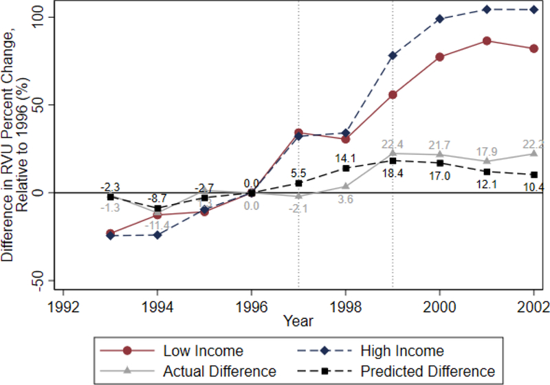
Notes: Data from the Federal Register and MCBS. This figure examines the difference in cumulative percent changes in RVU for high- and low-income patients. High (low) income patients are those with income above (below) the median, and we examine changes in the total utilization for the median patient within each income group. The red and blue lines show actual percent changes in utilization, relative to 1996 (akin to Figure 1), and the grey line shows their difference (i.e., high – low income percent changes). The black line is the difference in percent changes in predicted utilization, as extracted from our estimate of Equation (7).

According to the solid grey curve, actual utilization trends seem to take one or two years to respond to the Medicare policy shock. While the precise dynamics of how and when physicians respond to reimbursement changes remains beyond the scope of this paper, we note this general pattern is consistent with prior literature on the effects of Medicare reimbursement reforms (Clemens and Gottlieb 2014).¹⁹

5. Conclusion

In this paper, we present a model of decision-making by physicians with imperfect altruism towards their patients. We show that the same physician may respond differently to price changes when treating patients with different socioeconomic status. We compute the size and direction of this effect empirically: within-physician price elasticities vary from 0.02 to 0.18 across the 10^th and 90^th percentiles of the patient socioeconomic status distribution. On average, the Medicare policy shocks studied increase utilization by 10.4 percentage points more for higher income patients.

While our measures of price elasticities rely on plausibly exogenous variation, future research could study not only exogenous changes in reimbursement, but also natural experiments in patient socioeconomic status across physicians. In addition, we have taken as given that physicians choose treatments on behalf of their patients. In some cases, patients may have more influence over the outcome; such shared decision–making can be influenced by the length of the physician-patient relationship. The implications of the physician-patient relationship for price elasticity represent another fertile area for future research using longer-term data.

The health economics literature has long recognized the tension between physician altruism and physician profit-maximization, and in prior research, economists have developed elegant and tractable models accounting for this tension. We exploit these tools to investigate how patient socioeconomic status impacts pricing and utilization behavior in healthcare markets. Our analysis demonstrates that the unique preferences and objectives of physicians create price responses that vary across socioeconomic groups. Our empirical results provide guidance for policymakers and researchers. Heterogeneity in the effect of reimbursement changes is to be expected, and policymakers ought to account for the unequal effects of pricing reforms on patients in different socioeconomic strata. Suitably directed empirical analysis can help inform more targeted approaches to reforming reimbursement policy, particularly when the goal is to protect vulnerable socioeconomic groups.

Appendix A: Mathematical Appendix

We provide the detailed math accompanying propositions made in the paper. As laid out in the paper, we make the following assumptions:

$$u^{‴}=0, z^{″}=0, z^{‴}=0$$

$$F\prime \prime \langle 0, c\prime \prime \rangle 0$$

$$F\prime \prime \prime =0, c\prime \prime \prime =0$$

$${\sigma }_X>0, {\sigma }_P>0, {\sigma }_{XP}>0, {\sigma }_{XX}=0$$

Physicians maximize the following objective function:

$$\underset{X}{\max }\left(1-\alpha \right)z\left(PX-c\left(X\right)\right)+\alpha u\left(I+vF\left(X\right)-\pi -\sigma \left(X;P\right)\right)$$

The first-order condition is:

$$\alpha u^{\prime }*\left(vF\prime -{\sigma }_X\right)+\left(1-\alpha \right)z^{\prime }*\left(P-c\prime \right)=0$$

The comparative static of price on utilization is given by:

$$\frac{\partial X}{\partial P}=\frac{\left(-\alpha u^{\prime }{\sigma }_{XP}-\alpha u^{″}\left(vF\prime -{\sigma }_X\right)\left({\sigma }_P\right)+\left(1-\alpha \right)z^{\prime }+\left(1-\alpha \right)z^{″}\left(P-c\prime \right)X\right)}{\left(-D\right)},$$

where $D\equiv \alpha u^{″}{\left(vF\prime -{\sigma }_X\right)}^2+\alpha u^{\prime }\left(vF\prime \prime \right)+\left(1-\alpha \right)z^{″}{\left(P-c\prime \right)}^2+\left(1-\alpha \right)z^{\prime }\left(-c\prime \prime \right)<0$. Below, we prove Proposition 1 for when there is private over-use (case 1) and private under-use (case 2).

A.1. Case 1: Private Over-use: $\mathbf{v}F\prime -{\mathbf{\sigma }}_{\mathbf{X}}\mathbf{<}0$

In the case of private over-use, the effect of income on utilization is positive because

$\frac{\partial X}{\partial I}=\frac{\left[\alpha u^{″}\left(vF\prime -{\sigma }_X\right)\right]}{\left(-D\right)}>0$ Higher income results in higher medical care utilization. Next, we establish a few useful lemmas in the case of private over-use.

Useful Lemmas in the Case of Private Over-Use

Define:

$$N_P\equiv \left(-\alpha u^{\prime }{\sigma }_{XP}-\alpha u^{″}\left(vF\prime -{\sigma }_X\right)\left({\sigma }_P\right)+\left(1-\alpha \right)z^{\prime }+\left(1-\alpha \right)z^{″}\left(P-c\prime \right)X\right)$$

$$N_I\equiv \left[\alpha u^{″}\left(vF\prime -{\sigma }_X\right)\right]$$

Lemma 1: Prove: $\frac{\partial \left(-D\right)}{\partial X}>0$. Note that $\frac{\partial \left(-D\right)}{\partial X}$ has the following four components:

$${\mathrm{\Gamma }}_1^1\equiv -\alpha u^{‴}{\left(vF\prime -{\sigma }_X\right)}^3-\alpha u^{″}2\left(vF\prime -{\sigma }_X\right)\left(vF\prime \prime -{\sigma }_{XX}\right)>0$$

where this result follows because $u^{‴}\ge 0$, $u^{″}<0$, $F\prime <0$, and ${\sigma }_{XX}=0$.

$${\mathrm{\Gamma }}_2^1\equiv -\alpha u^{″}\left(vF\prime \prime \right)\left(vF\prime -{\sigma }_X\right)-\alpha u^{\prime }\left(vF\prime \prime \prime \right)>0$$

Where this result follows because $F_{XXX}\le 0$.

$${\mathrm{\Gamma }}_3^1\equiv -\left(1-\alpha \right)z^{‴}{\left(P-c^{\prime }\right)}^3-\left(1-\alpha \right)z\prime \prime 2\left(P-c\prime \right)\left(-c\prime \prime \right)$$

This term disappears under physician risk-neutrality.

$${\mathrm{\Gamma }}_4^1\equiv \left(1-\alpha \right)z^{″}\left(c\prime \prime \right)\left(P-c\prime \right)+\left(1-\alpha \right)z^{\prime }\left(c\prime \prime \prime \right)\ge 0$$

This result follows so long as $c\prime \prime \prime \ge 0$ and $z\prime \prime =0$. QED

Lemma 2: Prove: $\frac{\partial N_P}{\partial X}<0$

Note that $\frac{\partial N_P}{\partial X}$ has the following four components:

$${\mathrm{\Gamma }}_1^2\equiv -\alpha u^{″}{\sigma }_{xP}\left(vF\prime -{\sigma }_X\right)<0$$

This result follows by our case assumption.

$${\mathrm{\Gamma }}_2^2\equiv \frac{\partial \left(-\alpha u^{″}\left(vF\prime -{\sigma }_X\right)\left({\sigma }_P\right)\right)}{\partial X}=-\alpha u^{‴}{\left(vF\prime -{\sigma }_X\right)}^2{\sigma }_P-\alpha u^{″}\left(vF\prime \prime -{\sigma }_{XX}\right)\left({\sigma }_P\right)-\alpha u^{″}\left(vF\prime -{\sigma }_X\right){\sigma }_{PX}<0$$

This result follows so long as $u^{‴}\ge 0$.

$${\mathrm{\Gamma }}_3^2\equiv \left(1-\alpha \right)z^{″}\left(P-c\prime \right)\le 0$$

This result follows so long as $z^{″}\le 0$.

$${\mathrm{\Gamma }}_4^2\equiv \left(1-\alpha \right)z^{‴}{\left(P-c\prime \right)}^{2}X+\left(1-\alpha \right)z^{″}\left(P-c\prime -c\prime \prime X\right)=0$$

This follows because $z^{‴}=0$, and $z^{″}=0$. QED

Lemma 3: Prove: $\frac{\partial N_I}{\partial X}>0$

Note that $\frac{\partial N_I}{\partial X}=\alpha u^{″}\left(vF\prime \prime -{\sigma }_{XX}\right)+\alpha u^{‴}{\left(vF\prime -{\sigma }_X\right)}^2>0$. This proves the result, because $F\prime \prime <0$ and $u^{‴}\ge 0$. QED

Lemma 4: Prove: $\frac{\partial \left(-D\right)}{\partial I}<0$

Note that $\frac{\partial \left(-D\right)}{\partial I}=-\alpha u^{‴}{\left(vF\prime -{\sigma }_X\right)}^2-\alpha u^{″}\left(vF\prime \prime \right)$. Since $u^{‴}\ge 0$ and $u^{‴}<0$, this term is negative. QED

Lemma 5: Prove: $\frac{\partial N_P}{\partial I}>0$

$\frac{\partial N_P}{\partial I}=-\alpha u^{″}{\sigma }_{XP}-\alpha u^{‴}\left(vF\prime -{\sigma }_X\right)\left({\sigma }_P\right)>0$, because $u^{‴}<0$ and $u^{‴}\ge 0$. QED

Proof of Proposition 1 in the Case of Private Over-Use

We will now prove Proposition 1 for the private over-use case, or specifically: if $vF\prime -{\sigma }_X<0$ and $\frac{\partial X}{\partial P}>0$, then ${\frac{{\partial }^{2}X}{\partial P\partial I}|}_{X^{*}}>0$ and $\frac{{\partial }^{2}X}{\partial P\partial I}<{\frac{{\partial }^{2}X}{\partial P\partial I}|}_{X^{*}}$.

For fixed X,$\frac{{\partial }^{2}X}{\partial P\partial I}=\frac{\frac{\partial N_P}{\partial I}\left(-D\right)-\frac{\partial \left(-D\right)}{\partial I}\left(N_P\right)}{{\left(-D\right)}^2}$. Recall that $\frac{\partial N_P}{\partial I}>0$ and $\frac{\partial \left(-D\right)}{\partial I}<0$, and when $\frac{\partial X}{\partial P}>0$, it implies that $N_P>0$. This proves that ${\frac{{\partial }^{2}X}{\partial P\partial I}|}_{X^{*}}>0$.

Next, observe that the total change in the numerator of $\frac{\partial X}{\partial P}$ with respect to patient income is given by:$\frac{\partial N_P}{\partial X}\frac{\partial X}{\partial I}+\frac{\partial N_P}{\partial I}{\text{}|}_{X^{*}}$. Since $\frac{\partial N_P}{\partial X}<0$ and $\frac{\partial X}{\partial I}>0$, it follows that $\frac{\partial N_P}{\partial X}\frac{\partial X}{\partial I}+\frac{\partial N_P}{\partial I}{\text{}|}_{X^{*}}<{\frac{\partial N_P}{\partial I}|}_{X^{*}}$. Similarly, the total change in the denominator with respect to patient income is given by:$\frac{\partial \left(-D\right)}{\partial X}\frac{\partial X}{\partial I}+\frac{\partial \left(-D\right)}{\partial I}$. Since $\frac{\partial \left(-D\right)}{\partial X}$>0 and $\frac{\partial X}{\partial I}>0$, it follows that $\frac{\partial \left(-D\right)}{\partial I}>{\frac{\partial \left(-D\right)}{\partial I}|}_{X^{*}}$. QED

A.2. Case 2: Private Under-use: $\mathbf{v}F\prime -{\mathbf{\sigma }}_{\mathbf{X}}\mathbf{>}0$

In the case of private under-use, the effect of income on utilization is negative because:

$\frac{\partial X}{\partial I}=\frac{\left[\alpha u^{″}\left(vF\prime -{\sigma }_X\right)\right]}{\left(-D\right)}<0$

Next, we establish some useful lemmas in the case of private under-use.

Useful Lemmas in the Case of Private Under-Use

Define:

$$\begin{gathered} N_P\equiv \left(-\alpha u^{\prime }{\sigma }_{XP}-\alpha u^{″}\left(vF\prime -{\sigma }_X\right)\left({\sigma }_P\right)+\left(1-\alpha \right)z^{\prime }+\left(1-\alpha \right)z^{″}\left(P-c\prime \right)X\right) \\ {N}_I\equiv \left[\alpha u^{″}\left(vF\prime -{\sigma }_X\right)\right] \end{gathered}$$

Lemma 6: Prove:$\frac{\partial \left(-D\right)}{\partial X}<0$.

Note that $\frac{\partial \left(-D\right)}{\partial X}$ has the following four components:

$${\mathrm{\Gamma }}_1^1\equiv -\alpha u^{‴}{\left(v{F}^{\prime }-{\sigma }_X\right)}^3-\alpha u^{″}2\left(v{F}^{\prime }-{\sigma }_X\right)\left(v{F}^{″}-{\sigma }_{XX}\right)<0,$$

where this result follows because $u^{‴}\ge 0$, $u^{″}<0$, $F\prime \prime <0$, and ${\sigma }_{XX}=0$.

$${\mathrm{\Gamma }}_2^1\equiv -\alpha u^{″}\left(v{F}^{″}\right)\left(v{F}^{\prime }-{\sigma }_X\right)-\alpha u^{\prime }\left(v{F}^{‴}\right)<0,$$

where this result follows so long as $F\prime \prime \prime \ge 0$.

$${\mathrm{\Gamma }}_3^1\equiv -\left(1-\alpha \right)z^{‴}{\left(P-c\prime \right)}^3-\left(1-\alpha \right)z^{″}2\left(P-c\prime \right)\left(-c\prime \prime \right)<0$$

This result follows as long as $z^{‴}=z^{″}=0$.

$${\mathrm{\Gamma }}_4^1\equiv \left(1-\alpha \right)z^{″}\left(c\prime \prime \right)\left(P-c\prime \right)+\left(1-\alpha \right)z^{\prime }\left(c\prime \prime \prime \right)\le 0$$

This result follows so long as $c\prime \prime \prime \le 0$. QED

Lemma 7: Prove: $\frac{\partial N_P}{\partial X}>0$

Note that $\frac{\partial N_P}{\partial X}$ has the following four components:

$${\mathrm{\Gamma }}_1^2\equiv -\alpha u^{″}{\sigma }_{xP}\left(vF\prime -{\sigma }_X\right)>0$$

This result follows, so long as care is beneficial to consumers on the margin.

$${\mathrm{\Gamma }}_2^2\equiv \frac{\partial \left(-\alpha u^{″}\left(v{F}^{\prime }-{\sigma }_X\right)\left({\sigma }_P\right)\right)}{\partial X}=-\alpha u^{‴}{\left(vF\prime -{\sigma }_X\right)}^2{\sigma }_P-\alpha u^{″}\left(vF\prime \prime -{\sigma }_{XX}\right)\left({\sigma }_P\right)-\alpha u^{″}\left(vF\prime -{\sigma }_X\right){\sigma }_{PX}>0$$

Under our assumption that $u^{‴}\le 0$, the result follows.

$${\mathrm{\Gamma }}_3^2\equiv \left(1-\alpha \right)z^{″}\left(P-c\prime \right)\ge 0$$

This result follows from $z^{″}\le 0$

$${\mathrm{\Gamma }}_4^2\equiv \left(1-\alpha \right)z^{‴}{\left(P-c\prime \right)}^{2}X+\left(1-\alpha \right)z^{″}\left(P-c\prime -c\prime \prime X\right)>0$$

This follows because $z^{‴}\ge 0$, and $z^{″}\le 0$. QED

Lemma 8: Prove: $\frac{\partial N_I}{\partial X}>0$

Note that $\frac{\partial N_I}{\partial X}=\alpha u^{″}\left(vF\prime \prime -{\sigma }_{XX}\right)+\alpha u^{‴}{\left(vF\prime -{\sigma }_X\right)}^2>0$. This proves the result, because $F\prime \prime \le 0$ and $u^{‴}\ge 0$. QED

Lemma 9: Prove: $\frac{\partial \left(-D\right)}{\partial I}<0$

Note that $\frac{\partial \left(-D\right)}{\partial I}=-\alpha u^{‴}{\left(vF\prime -{\sigma }_X\right)}^2-\alpha u^{″}\left(vF\prime \prime \right)$. Since $u^{‴}\ge 0$ and $F\prime \prime <0$, this term is negative. QED

Lemma 10: Prove: $\frac{\partial N_P}{\partial I}>0$

$\frac{\partial N_P}{\partial I}=-\alpha u^{″}{\sigma }_{XP}-\alpha u^{‴}\left(vF\prime -{\sigma }_X\right)\left({\sigma }_P\right)>0$. This result follows if $u^{‴}=0$. QED

Proof of Proposition 1 in the Case of Private Under-Use

We will now prove Proposition 1 for the private under-use case, or specifically: If $vF\prime -{\sigma }_X>0$ and $\frac{\partial X}{\partial P}>0$, then then ${\frac{{\partial }^{2}X}{\partial P\partial I}|}_{X^{*}}>0$ and $\frac{{\partial }^{2}X}{\partial P\partial I}<{\frac{{\partial }^{2}X}{\partial P\partial I}|}_{X^{*}}$.

For fixed X,$\frac{{\partial }^{2}X}{\partial P\partial I}=\frac{\frac{\partial N_P}{\partial I}\left(-D\right)-\frac{\partial \left(-D\right)}{\partial I}\left(N_P\right)}{{\left(-D\right)}^2}$. Recall that $\frac{\partial N_P}{\partial I}>0$ and $\frac{\partial \left(-D\right)}{\partial I}<0$, and when $\frac{\partial X}{\partial P}>0$, it implies that $N_P>0$. This proves that ${\frac{{\partial }^{2}X}{\partial P\partial I}}_{X^{*}}>0$.

Next, observe that the total change in the numerator of $\frac{\partial X}{\partial P}$ with respect to patient income is given by:$\frac{\partial N_P}{\partial X}\frac{\partial X}{\partial I}+\frac{\partial N_P}{\partial I}{\text{}|}_{X^{*}}$. Since $\frac{\partial N_P}{\partial X}>0$ and $\frac{\partial X}{\partial I}<0$, it follows that $\frac{\partial N_P}{\partial X}\frac{\partial X}{\partial I}+\frac{\partial N_P}{\partial I}{\text{}|}_{X^{*}}<{\frac{\partial N_P}{\partial I}|}_{X^{*}}$. Similarly, the total change in the denominator with respect to patient income is given by:$\frac{\partial \left(-D\right)}{\partial X}\frac{\partial X}{\partial I}+\frac{\partial \left(-D\right)}{\partial I}$. Since $\frac{\partial \left(-D\right)}{\partial X}$<0 and $\frac{\partial X}{\partial I}<0$, it follows that $\frac{\partial \left(-D\right)}{\partial I}>{\frac{\partial \left(-D\right)}{\partial I}|}_{X^{*}}$. QED

Appendix B: Empirical Appendix

In this section, we further illustrate the distribution of price variation from our GAF and PE-RVU instruments, shown in Figures B1 and B2, and we discuss the remaining policy changes during 1992 to 2003 that affected Medicare payments. We also document our construction of the health variables.

Variation in Medicare Payments

Other than the GAF and PE-RVU components detailed in Section 3.2, variation in Medicare payments come from changes in the work RVU, malpractice RVU, and CF. On average, work RVUs, PE-RVUs, and malpractice RVUs account for 52 percent, 44 percent, and 4 percent of total payments, respectively (US Government Accountability Office, 2005). Because the malpractice component accounts for such a small share of payments, we do not focus on it.

From 1993 to 2002, work RVUs experienced two major reviews which became effective in 1997 and 2002. Plot (a) of Figure B3 shows the average work RVU over time for HCPCS. After the RUC committee met to re-assess work RVUs, we see clear jumps in the RVU. However, with competing political pressures and physician incentives, it is unlikely that RUC committee changes are exogenous to local demand and supply factors.

The change in methodology for determining practice expense RVUs (PE-RVUs) from a charge-based method to a resource-based system was enacted by the Balance Budget Act of 1997. In developing the resource-based system, CMS considered the staff equipment and supplies used in providing medical and surgical services in various settings (Federal Register 1999). A new set of RVUs were proposed in June 1997 and subsequently adjusted following the review of approximately 8,600 comments from providers and professional associations and societies. From 1999 to 2002, the new PE-RVU system was phased in as follows: in 1999 PE-RVUs were calculated as a product of 75% of the previous charge-based PE-RVUs and 25% of the resource-based PE-RVU system. In 2000, the percentages were 50% of the charge-based system and 50% of the resource-based system. In 2001, the percentages were 25% of the charge-based system and 75% of the resource-based system. By 2002, PE-RVUs were based totally on resource-based expenses.

The CF also experienced a major change during our study period. Prior to 1998, there were three different CFs: one for surgery, primary care, and non-surgical services. The CF for surgical procedures led to surgeons earning a 17 percent bonus payment relative to all other procedures. This generated political discontent and led to a budget-neutral merger of CFs in 1998 (Clemens and Gottlieb, 2013). Plot (b) shows the CFs over time. After 1998, the CF for surgical procedures fell by about 11 percent, whereas the CF for non-surgical procedures increased by about 6 percent. We do not use this policy shock as another instrument for two reasons. First, CFs are constant across all geographic regions and all procedures, so their explanatory power for payment changes within physicians is weak. Second, the shock in CF payments occurs mainly for surgical procedures, while changes in CF for non-surgical and primary care procedures are much less pronounced.

Construction of Health Variables

Measures of underlying health are extracted from claims and survey data. From the claims data, we calculate the Charlson Comorbidity Index, which reflects the cumulative increase in likelihood of one-year mortality due to the severity of comorbidities (Quan et al. 2005). (Quan et al. 2005) From the survey data, we utilize self-reported metrics of height and weight to calculate body mass index. We also created eight indicator variables for:

• Broken hip, which equals one if the individual has had a broken hip within the last year.

• Cancer, which equals one if the individual has any of the following cancers: bladder, breast, cervical, colon, head, kidney, lung, ovarian, prostate, stomach, throat, uterine or other cancer.

• Diabetes, which equals one if the individual has diabetes.

• Heart disease, which equals one if the individual has coronary heart disease, a myocardial infarction, or other heart conditions.

• Hypertension, which equals one if the individual has hypertension.

• Lung disease, which equals one if the individual has asthma, chronic obstructive pulmonary disease, or emphysema.

• Neurological disease, which equals one if the individual has Alzheimer’s, Parkinson’s, a stroke, or other psychiatric condition (but excluding mental retardation).

• Some difficulty in physical functioning, which equals one if the individual has some or more difficulty in executing at least one of five activities: stooping or crouching; lifting or carrying objects of up to 10 pounds, extending arms above the shoulder; grasping small objects; and walking two or three blocks.

Figure B1.

Practice Expense RVU by Facility

Notes: Data from the Federal Register 1992–2003. The top line shows changes in the facility PE-RVU. The bottom line shows changes in the non-facility PE-RVU. Sample restricted to HCPCS observed in all years.

Figure B2.

Distribution of Instrument-Induced Price Shocks

Notes: Data from the Federal Register and MCBS at the physician-patient-year level. Plot (a) shows the distribution of the GAF-induced price change from 1996 to 1997. Plot (b) shows the distribution of PE-RVU induced price changes for physician baskets of goods from 1998 to 2002.

Figure B3.

Percent Change in PE-RVU Across HCPCS

Notes: Data from the Federal Register and MCBS. For each HCPCS, we calculate the aggregate percent change in PE-RVU from 1998 to 2002. The histogram of changes across procedures are shown.

Figure B4.

Remaining Variation in Medicare Payments

Notes: Data from Federal Register 1992–2003. Plot (a) show the change in work-RVUs. Evident from the graph are the two major reviews by the RUC committee in 1997 and 2002. The sample is restricted to HCPCS observed in all years. Plot (b) shows the change from three CFs (primary care, surgical, and non-surgical) to a single budget-neutral CF in 1998.

REFERENCES

- Aiken Leona S, and West Stephen G 1991. Multiple Regression Testing and Interpreting Interactions (Sage Publications: Thousand Oaks, CA: ). [Google Scholar]
- Altonji Joseph G, Elder Todd E, and Taber Christopher R 2005. ‘Selection on Observed and Unobserved Variables: Assessing the Effectiveness of Catholic Schools’, Journal of Political Economy, 113: 151–84. [Google Scholar]
- Arrow Kenneth J. 1963. ‘Uncertainty and the Welfare Economics of Medical Care’, American Economic Review, 53: 941–73. [Google Scholar]
- Becker Gary. 1957. The Economics of Discrimination (The University of Chicago Press: Chicago, IL: ). [Google Scholar]
- Becker Gary S, and Murphy Kevin M 1988. ‘A Theory of Rational Addiction’, Journal of Political Economy, 96: 675–700. [Google Scholar]
- Blomqvist Ake. 2002. ‘Defining the Value of a Statistical Life: A Comment’, J Health Econ, 21: 169–75. [DOI] [PubMed] [Google Scholar]
- Chew SH, Epstein LG, and Segal U 1991. ‘Mixture Symmetry and Quadratic Utility’, Econometrica, 59: 139–63. [Google Scholar]
- Chone Philippe, and Ching-to Albert Ma. 2011. ‘Optimal Health Care Contract under Physician Agency’, Annals of Economics and Statistics: 229–56.
- Clemens Jeffrey, and Gottlieb Joshua D. 2014. ‘Do Physicians’ Financial Incentives Affect Medical Treatment and Patient Health?()’, The American Economic Review, 104: 1320–49. [DOI] [PMC free article] [PubMed] [Google Scholar]
- Dickstein Michael 2016. ‘Patient vs. Patient Incentives in Prescription Drug Choice’, Working Paper
- Donahue Katrina E., Ashkin Evan, and Pathman Donald E. 2005. ‘Length of patient-physician relationship and patients’ satisfaction and preventive service use in the rural south: a cross-sectional telephone study’, BMC Family Practice, 6: 40–40. [DOI] [PMC free article] [PubMed] [Google Scholar]
- Dranove D, and White WD 1987. ‘Agency and the organization of health care delivery’, Inquiry, 24: 405–15. [PubMed] [Google Scholar]
- Dranove David 1988. ‘Demand Inducement and the Physician/Patient Relationship’, Economic Inquiry, 26: 281–98. [DOI] [PubMed] [Google Scholar]
- Ellis RP, and McGuire TG 1990. ‘Optimal payment systems for health services’ [DOI] [PubMed]
- Ellis Randall P., and McGuire Thomas G. 1986. ‘Provider behavior under prospective reimbursement: Cost sharing and supply’, J Health Econ, 5: 129–51. [DOI] [PubMed] [Google Scholar]
- Emanuel EJ, and Emanuel LL 1992. ‘Four models of the physician-patient relationship’, JAMA, 267: 2221–26. [PubMed] [Google Scholar]
- Evans William N., and Kip Viscusi W 1993. ‘Income Effects and the Value of Health’, The Journal of Human Resources, 28: 497–518. [Google Scholar]
- Fairbrother Gerry, Jain Aparna, Park Heidi L, Massoudi Mehran S, Arfana Haidery, and Gray Bradford H. 2004. ‘Churning in Medicaid Managed Care and Its Effect on Accountability’, Journal of Health Care for the Poor and Underserved, 15: 30–41. [DOI] [PubMed] [Google Scholar]
- Federal Register. 1999. “Medicare Program; Payment Policies Under Physician Fee Schedule for Calendar Year 2000.” In 42 CFR Parts 410, 411, 414, 415, and 485, edited by Department of Health and Human Services. [Google Scholar]
- Finkelstein Amy, Luttmer Erzo F. P., and Notowidigdo Matthew J. 2013. ‘What Good is Wealth Without Health? The Effect of Health on the Marginal Utility of Consumption’, Journal of the European Economic Association, 11: 221–58. [Google Scholar]
- Glied Sherry, and Joshua Graff Zivin 2002. ‘How do doctors behave when some (but not all) of their patients are in managed care?’, J Health Econ, 21: 337–53. [DOI] [PubMed] [Google Scholar]
- Godager Geir, and Wiesen Daniel 2013. ‘Profit or patients’ health benefit? Exploring the heterogeneity in physician altruism’, J Health Econ, 32: 1105–16. [DOI] [PubMed] [Google Scholar]
- Gruber Jonathan (ed.)^(eds.). 2013. Proposal 3: Restructuring Cost Sharing and Supplemental Insurance for Medicare (Brookings; ). [Google Scholar]
- Hansen Lars Peter 1982. ‘Large Sample Properties of Generalized Method of Moments Estimators’, Econometrica, 50: 1029–54. [Google Scholar]
- Hayashi Fumio 2000. Econometrics (Princeton University Press: Princeton, NJ: ). [Google Scholar]
- Jack William 2005. ‘Purchasing health care services from providers with unknown altruism’, J Health Econ, 24: 73–93. [DOI] [PubMed] [Google Scholar]
- Jacobson Mireille G., Chang Tom Y., Earle Craig C., and Newhouse Joseph P. 2017. ‘Physician Agency and Patient Survival’, Journal of Economic Behavior & Organization, 134: 27–47. [DOI] [PMC free article] [PubMed] [Google Scholar]
- Klaiber H. Allen, and von Haefen Roger H. 2018. ‘Do Random Coefficients and Alternative Specific Constants Improve Policy Analysis? An Empirical Investigation of Model Fit and Prediction’, Environmental and Resource Economics: 1–17.
- Lillard Lee A., and Weiss Yoram 1997. ‘Uncertain Health and Survival: Effects on End-of-Life Consumption’, Journal of Business & Economic Statistics, 15: 254–68. [Google Scholar]
- Liu Ting, and Ching-to Albert Ma. 2013. ‘Health insurance, treatment plan, and delegation to altruistic physician’, Journal of Economic Behavior & Organization, 85: 79–96. [Google Scholar]
- MaCurdy Thomas, Shafrin Jason, Thomas DeLeire Jed DeVaro, Bounds Mallory, Pham David, and Chia Arthur 2012. Geographic Adjustment of Medicare Payments to Physicians: Evaluation of IOM Recommendations (Acumen, LLC: Burlingame, CA: ). [Google Scholar]
- Maxwell Stephanie, and Zuckerman Stephen 2007. ‘Impact of Resource-Based Practice Expenses on the Medicare Physician Volume’, Health Care Financing Review, 29: 65–79. [PMC free article] [PubMed] [Google Scholar]
- McGuire Thomas G. 2000. ‘Physician Agency.’ in A. Culyer J, Newhouse JP (ed.), Handbook of Health Economics (Elsevier Science B.V.). [Google Scholar]
- McGuire Thomas G., and Pauly Mark V. 1991. ‘Physician Response to Fee Changes with Multiple Payers’, J Health Econ, 10: 385–410. [DOI] [PubMed] [Google Scholar]
- Mooney G, and Ryan M 1993. ‘Agency in health care: getting beyond first principles’, J Health Econ, 12: 125–35. [DOI] [PubMed] [Google Scholar]
- Olea José Luis Montiel, and Pflueger Carolin 2013. ‘A Robust Test for Weak Instruments’, Journal of Business & Economic Statistics, 31: 358–69. [Google Scholar]
- Oster Emily 2016. ‘Unobservable Selection and Coefficient Stability: Theory and Evidence’, Journal of Business & Economic Statistics: 1–18.
- Quan H, Sundararajan V, Halfon P, Fong A, Burnand B, Luthi JC, Saunders LD, Beck CA, Feasby TE, and Ghali WA 2005. ‘Coding algorithms for defining comorbidities in ICD-9-CM and ICD-10 administrative data’, Medical Care, 43: 1130–9. [DOI] [PubMed] [Google Scholar]
- Rochaix Lise 1989. ‘Information asymmetry and search in the market for physicians’ services’, J Health Econ, 8: 53–84. [DOI] [PubMed] [Google Scholar]
- Sargan JD 1958. ‘The Instability of the Leontief Dynamic Model’, Econometrica, 26: 381–92. [Google Scholar]
- Sommers Benjamin D., and Rosenbaum Sara 2011. ‘Issues In Health Reform: How Changes In Eligibility May Move Millions Back And Forth Between Medicaid And Insurance Exchanges’, Health Affairs, 30: 228–36. [DOI] [PubMed] [Google Scholar]
- Staiger Douglas O., and Stock James H. 1997. ‘Instrumental Variables Regression with Weak Instruments’, Econometrica, 65: 557–86. [Google Scholar]
- Stock James H., and Yogo Motohiro 2005. ‘Testing for Weak Instruments in Linear IV Regression.’ in Donald W.K. Andrews and Stock James H. (eds.), Identification and Inference for Econometric Models (Cambridge University Press: Cambridge, UK: ). [Google Scholar]
- Zweifel Peter, Breyer Friedrich, and Kifmann Mathias 1997. Health Economics (Oxford University Press: New York, NY: ). [Google Scholar]