A Commentary on Diversity Measures UniFrac in Very Small Sample Size

Abstract

In phylogenetic, the diversity measures as UniFrac, weighted UniFrac, and normalized weighted UniFrac are used to estimate the closeness between two samples of genetic material sequences. These measures are widely used in microbiology to compare microbial communities. Furthermore, when the sample size is large enough, very good results have been obtained experimentally. However, some authors do not suggest using them when the sample size is very small. Recently, it has been mentioned that the weighted UniFrac measure can be seen as the Kantorovich-Rubinstein metric between the corresponding empirical distributions of samples of genetic material. Also, it is well known that the Kantorovich-Rubinstein metric complies the metric definition. However, one of the main reasons to establish it is that the sample size is large enough. The goal of this article is to prove that the diversity measures UniFrac are not metrics when the sample size is very small, which justifies why it must not be used in that case, but yes the Kantorovich-Rubinstein metric.

Introduction

Phylogenetic is a field of biology that studies how organisms are related during evolution. The basic principle is that the members of an organism set that descend from the same ancestor share an evolutionary history. A problem in phylogenetic analysis is to determine similarities and differences between genetic material sequences. For example, the study of the degree of difference between two samples A and B of genetic material sequences. For this, the diversity measure UniFrac,¹ weighted UniFrac and normalized weighted UniFrac² have been used.

The above diversity measures are used by several authors in microbiology field to compare genetic material samples. For example, Frank et al³ said the diversity measure UniFrac is used to check whether patients with inflammatory bowel disease present samples from different microbial communities to patients without the disease. According to Costello et al,⁴ the weighted UniFrac and normalized weighted UniFrac are used to better understand the structure of the microbial community in skin sites and other body habitats between different individuals and at different times, and it is suggested that these trends may reveal how changes in the microbial cause or prevent diseases. Another application of these measures is given in Charlson et al,⁵ which are used to compare the population of bacteria in the lungs and their relationship with the population of bacteria of the upper respiratory tract, the former in healthy individuals. On the other hand, Ley et al⁶ said the diversity measure was used to measure the difference between bacterial communities in mice intestines, in order to test the effects of kinship and genotype diversity.

Moreover, from the theoretical point of view, diversity measures UniFrac give rise to other measures, for example, Chang et al⁷ proposed a new weighting scheme assuming that the sequences are randomly distributed; this scheme is called weighted UniFrac adjusted variance (VAW-UniFrac) and it is proposed as an improvement of weighted UniFrac. Furthermore, the VAW-UniFrac measure is compared to the UniFrac and weighted UniFrac measures to determine which is more efficient. Chen et al⁸ gave a generalization of the UniFrac diversity measures, this generalization is more usefulness to detect a set of biologically relevant changes than the UniFrac measure.

However, despite its practical application in the microbiology field, in Schloss,⁹ it is mentioned that ‘A recent simulation study concluded that UniFrac is unsuitable as a distance metric and should not be used for multivariate analysis’ that means, it is not appropriate to use diversity measures UniFrac as metrics and they should not be used in multivariate analysis.

Recently, in Evans and Matsen¹⁰ was mentioned that the weighted UniFrac measure is the classical Kantorovich-Rubinstein metric^11–14 or Earth Mover Distance¹⁵ between the corresponding empirical distribution of samples of genetic material on a phylogenetic tree. The above, under assumption that the sample size is large enough. In this way, McClelland and Koslicki¹⁶ propose the earth mover distance UniFrac (EMDUniFrac) and an algorithm to compute it.

In this article, we proof that the original version of diversity measures UniFrac are not metrics but they are pseudosemimetrics. They satisfy the following definition.

Definition 1

Let $X$ be a set, a function $d:X\times X\to [0,+\infty )$ is a pseudosemimetric in $X$ if for all $x,y\in X$ the function $d$ satisfies

1. If $x=y$, then $d(x,y)=0$.

2. $d(x,y)=d(y,x)$.

The above justifies why UniFrac measures can behave unexpectedly for small samples in multivariate data analysis, but it is not the case when the sample size is large enough. Thus, when the sample size is very small, it is recommended to use EMDUniFrac metric.

The rest of the work is developed as follows. In section “Rooted phylogenetic trees,” the necessary concepts will be given to define diversity measures. In section “Diversity measures UniFrac,” the three versions are defined: UniFrac, weighted UniFrac, and normalized weighted UniFrac, and we will show that they are pseudo-parametric; in this way, we prove that they are not metrics and how they are susceptible to small samples. In section “EMDUniFrac,” the UniFrac measures are estimated for some examples and they are compared with EMDUniFrac metric. Finally, some conclusions will be presented in section “Conclusions.”

Rooted Phylogenetic Trees

The diversity measures are calculated on a given phylogenetic tree. In this section, the concepts related to trees will be defined. They will be useful to address diversity measures UniFrac.

Basic definitions

Warnow¹⁷ defines a tree as a connected graph without cycles. A rooted tree $T$ is a tree in which a vertex $r$ is designated as root. The root in phylogenetic represents the common ancestor in the species represented in the tree $T$. The vertices represented the characteristics that allow to establish the similarities between different species. These characteristics are given by genetic material sequences.

The vertex $w$ is parent of $v$ and $v$ is a child of $w$, if $w$ and $v$ are vertices in the rooted tree $T$ such that $v\to w$. Moreover, a vertex $l$ is a leaf if $l$ does not have any children and $T$ is a binary tree if it has vertices with at most two children.

On the other hand, in a tree $T$, a path from vertex $x$ to vertex $y$ is the sequence of vertices in the graph such that there exist an edge between the vertex $x$ and the next one and so on until $y$, denoted by $[x,y]$. A branch $i$ is the vertices set and edges that belong to the path that goes from the leaf $l_i$ to the root $r$. We call leaf set of $T$ to the set $S$ built with different labels that are assigned to tree leaves $T$ and denoted by $L(T)$. Additionally, a clade of $T$ is a subset $A$ in $L(T)$ that it contains the leaf set of a subtree $T$, with root in some vertex $v\in T$ and it is denoted by $L(T_v)$ and $C(T)$ is the clades set $L(T_v)$ such that $v\in T$. The set $C(T)$ contains all the singular sets of leaves, a set that contains all the leaves and a clade for each remaining vertex of $T$.

Otherwise, Warnow¹⁷ associated the parameter $p(e)$ to the edge $e\in T$ where $p(e)$ denotes the probability of changing state where $0<p(e)<0.5$. A model tree Cavender-Farris-Neyman (CFN) is a pair $(T,\theta )$ where $T$ is a binary rooted tree with leaf set $\{l_1,\dots ,l_2\}$ and $\theta$ gives the $p(e)$ values for all edges $e\in T$. Under the CFN model, the number of changes in an edge is modeled by a Poisson random variable with expected value $\lambda (e)$. Then, instead of using the probability substitution $p(e)$ in each edge, we will use $\lambda (e)$, with the condition that $0<\lambda (e)$ for all $e$.

Thus, the branch length $i$, denoted by $d(l_i)$, is a positive number that represents the rate of change between the root $r$ and the leaf $l_i$, it is

$$d(l_i)=\sum _{e\in [r,l_i]}\lambda (e)$$

Let ${\lambda }_{[ij]}$ be the expected number of changes on the way $[l_i,l_j]$ on the tree $T$, it follows that

$${\lambda }_{[ij]}=\sum _{e\in [l_i,l_j]}\lambda (e)$$

We can see by the definition that $\lambda$ is the matrix distance on the road in a tree, where the path distance between two leaves is the sum of branch length and all branch lengths are positive. The matrix $\lambda$ is an additive matrix, which is defined as follows.

Definition 2

A matrix $M_{n\times n}$ is additive if there is a three $T$ with leaf set $\{l_1,\dots ,l_n\}$ and the lengths of the edges are non-negative, that is branch length of $[l_i,l_j]$ in $T$ is equal to $M_{[l_i,l_j]}$.

Phylogenetic tree construction

To construct a binary rooted phylogenetic tree using two samples $A$ and $B$, it is necessary to consider the partial order definition.

Definition 3

A partial order is a binary relation $R$ in a set $S$ such that for any $a,b,c\in S$ satisfies

1. Transitivity: $〈a,b〉\in R$ and $〈b,c〉\in R$ imply that $〈a,c〉\in R$.

2. Reflexivity: $〈a,a〉\in R\forall a\in R$.

3. Antisymmetry: $〈a,b〉\in R$ and $〈b,a〉\in R$ imply that $a=b$.

Two elements $a$ and $b$ are compatible if $〈a,b〉\in R$ or $〈b,a〉\in R$.

Hasse diagram is a graphic scheme of a partially ordered set. To construct the Hasse diagram of a set, a vertex is created for each element of $S$ and a directed edge $x\to y$ if $〈x,y〉\in R$ and x ≠ y. They are sorted from bottom to top, so the directed edges go up. The directed edges are removed $x\to y$ if there is a third vertex $z$ such that $〈x,z〉\in R$ and $〈z,y〉\in R$.

Let $T$ be a rooted phylogenetic tree and the clades set $C(T)$. The sequences $A$ and $B$ of genetic material are in relation, if $〈A,B〉\in R$ if and only if $A\subset B$. We can see that the relation $R$ is partial order.

Now, we will construct the Hasse diagram by $C(T)$ set. A graph is made assigning a vertex for each element in the set $C(T)$ and a directed edge from vertex $A$ to different vertex $B$ if $A\subset B$. The smallest subset $B$ must be found, and if $A\subset B$, we put a directed edge from $A$ to $B$. As containment is transitive, if $A\subset B$ and $B\subset C$, so $A\subset C$. Therefore, if there are directed edges from $A$ to $B$ and from $B$ to $C$ so there are edges from $A$ to $C$, and we can remove the directed edge from $A$ to $C$ without losing information.

The next theorem say that a binary rooted tree $T$ is isomorphic to the Hasse diagram built by $C(T)$. It is proven by Warnow.¹⁷

Theorem 1

Let $T$ be a rooted tree in which each internal node has two children. Then the Hasse diagram built by $C(T)$ is isomorphic to $T$. In this way, we can get the binary rooted tree $T$ from Hasse diagram built using the set $C(T)$.

In the next section, the diversity measures are addressed in their three versions, UniFrac, weighted UniFrac, and normalized weighted UniFrac. Also, we will show that they satisfy the pseudosemimetric definition and we will give examples where diversity measures do not satisfy the metric definition.

Diversity Measures UniFrac

To define the diversity measures UniFrac, it is considered a binary rooted phylogenetic tree $T$ for two samples $A$ and $B$ of genetic material sequences, where sample $A$ has $A_t$ sequences and sample $B$ has $B_t$ sequences, not necessarily different, that means that $A\cap B\ne \varnothing$ may occur and in each sample could be two or more equal sequences; furthermore, each sample can contain the root or not (common ancestor between species $A$ and $B$). Let $T$ be the tree with $n$ branches and let $d(l_i)$ be the length for each branch, with $i=1,\dots ,n$, they coincide with the distance from the root ($r$) to the sequence ($l_i$) that is in the leaf on $ith$ branch.

Let $A_i$ be the number of vertices in A that are in branch $i$, analogously, $B_i$ the number of vertices in $B$ that are in branch $i$ We define

$$P_i^A=\frac{A_i}{A_t}\mathrm{and}{P}_i^B=\frac{B_i}{B_t}$$

note that they are the proportions of descendant sequences in samples $A$ and $B$ in the $i$ branch, respectively.

Example 1

Consider the rooted tree in Figure 1. It is constructed using samples $A=\{r,a_1,a_1,a_2\}$ and $B=\{r,b_1,b_2\}$, where $A_t=4$ and $B_t=3$. The first branch has the sequences $r$ and $b_1$, where $r\in A$ and $\{r,b_1\}\in B$, so the proportion of descendant sequences in samples $A$ and $B$ on branch 1 are

Figure 1.

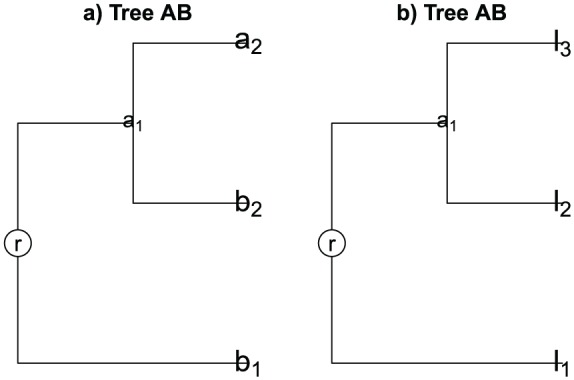
(a) Tree for samples $A$ and $B$. (b) Tree for samples $A$ and $B$ with the label leaves for $l_i$ with $i=1,2,3$ ($b_1=l_1,b_2=l_2,a_2=l_3$).

$$P_1^A=\frac{1}{4}\mathrm{and}{P}_1^B=\frac{2}{3}$$ (1)

respectively. The second branch has the sequences $r,a_1,b_2$ where $\{r,a_1,a_1\}\in A$ and $\{r,b_2\}\in B$, in this way

$$P_2^A=\frac{3}{4}\mathrm{and}{P}_2^B=\frac{2}{3}$$

analogously, the proportions of descendant sequences in third branch are

$$P_3^A=\frac{4}{4}\mathrm{and}{P}_3^B=\frac{1}{3}$$

In later examples, the sequences in leaf on the $ith$ branch will be denoted by $l_i$ (see Figure 1) in order to follow the given notation. This is because to definite the diversity measures, we need the branch length ($d(l_i)$) whose notation is given for sequences in the $ith$ leaf.

UniFrac

The diversity measure UniFrac was proposed by Lozupone and Knight¹ and it is defined as

$$d^u(A,B)=\frac{{\sum }_{i=1}^{n}d(l_i)|I(P_i^A>0)-I(P_i^B>0)|}{{\sum }_{i=1}^{n}d(l_i)}$$ (2)

where $I(\cdot )$ is the indicator function. We can see that the absolute value is $0$ or $1$. It is $1$ when the $ith$ branch has sequences in samples $A$ or $B$ and it is $0$ when has two samples.

Example 2

Consider the raised tree in Example 1, with $i=1,2,3$. The proportion of descendant sequences in $A$ and $B$ are greater than $0$, see the expression (1), then

$$I(P_i^A>0)=1\mathrm{and}I(P_i^B>0)=1$$

thus,

$$|I(P_i^A>0)-I(P_i^B>0)|=0$$

The diversity measure UniFrac version ignores the abundant information about sequences, only consider its presence or absence in the branch.

Proposition 1

The diversity measure UniFrac is a pseudosemimetric.

Proof

We will prove that the diversity measure UniFrac satisfies Definition 1. Moreover, we will give an example where it does not satisfy the metric definition.

1. If $A=B$, it is $A_i=B_i$ for all $i$ and $A_t=B_t$, so

$$I(P_i^A>0)=I(P_i^B>0)$$

for all $i$, thus,

$$|I(P_i^A>0)-I(P_i^B>0)|=0$$

therefore,

$$d^u(A,B)=0$$

• 2. To prove symmetry, we consider

$$\begin{array}{c}{d}^u(A,B)=\frac{{\sum }_{i=1}^{n}d(l_i)|I(P_i^A>0)-I(P_i^B>0)|}{{\sum }_{i=1}^{n}d(l_i)}\\ =\frac{{\sum }_{i=1}^{n}d(l_i)|I(P_i^B>0)-I(P_i^A>0)|}{{\sum }_{i=1}^{n}d(l_i)}\\ =d^u(B,A)\end{array}$$

Then the diversity measure UniFrac satisfies Definition 1. Additionally, we will give an example that does not satisfy the metric definition.

1. Let $T_{AB}$ be the tree built from two different samples:

$$A=\{r,l_1\}\mathrm{and}B=\{r,l_2\}$$

where $r$ is the root and the sequence l₁ ≠ l₂ (see Figure 2). The branch is the path from $r$ to $l_1$ and the branch $2$ the path from $r$ to $l_2$, we have to

Figure 2.

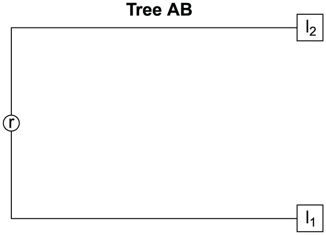
Tree for samples $A$ and $B$.

$$d^u(A,B)=\frac{d(l_1)|1-1|+d(l_2)|1-1|}{d(l_1)+d(l_2)}=0$$

however, we supposed that l₁ ≠ l₂. So that if $d^u(A,B)=0$, it does not imply that $A=B$.

• 2. We consider the samples

$$A=\{r,a\},B=\left\{b\right\}\mathrm{and}C=\{r,c\}$$

and the trees $T_{AB}$, $T_{AC}$, and $T_{CB}$ built for samples $A$ and $B$, $A$ and $C$, and $C$ and $B$, respectively (see Figure 3), where

Figure 3.

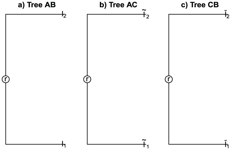
(a) Tree for samples $A$ and $B$. (b) Tree for samples $A$ and $C$. (c) Tree for samples $C$ and $B$.

$$l_1={\widehat{l}}_1=a,l_2={\overline{l}}_2=b\mathrm{and}{\widehat{l}}_2={\overline{l}}_1=c$$

Moreover, suppose that

$$d({\overline{l}}_1)<d(l_1)$$ (3)

If we estimate $d^u(A,B)$, $d^u(A,C)$, and $d^u(C,B)$ we have the following:

$$\begin{array}{c}{d}^u(A,B)=\frac{d(l_1)|1-0|+d(l_2)|1-1|}{d(l_1)+d(l_2)}\\ =\frac{d(l_1)}{d(l_1)+d(l_2)}\end{array}$$ (4)

$$\begin{array}{c}{d}^u(A,C)=\frac{d({\widehat{l}}_1)|1-1|+d({\widehat{l}}_2)|1-1|}{d({\widehat{l}}_1)+d({\widehat{l}}_2)}\\ =\frac{0}{d({\widehat{l}}_1)+d({\widehat{l}}_2)}=0\end{array}$$ (5)

$$\begin{array}{c}{d}^u(C,B)=\frac{d({\overline{l}}_1)|1-0|+d({\overline{l}}_2)|1-1|}{d({\overline{l}}_1)+d({\overline{l}}_2)}\\ =\frac{d({\overline{l}}_1)}{d({\overline{l}}_1)+d({\overline{l}}_2)}\end{array}$$ (6)

If the triangle inequality is satisfied and we considered expressions (4) to (6), we have that

$$\frac{d(l_1)}{d(l_1)+d(l_2)}\le 0+\frac{d({\overline{l}}_1)}{d({\overline{l}}_1)+d({\overline{l}}_2)}$$

where not necessary

$$d(l_1)<\_d({\overline{l}}_1)$$

It contradicts assumption (3). Then, triangle inequality is not satisfied.

Weighted UniFrac

The weighted UniFrac was proposed by Lozupone et al² and is denoted by

$$d^w(A,B)=\sum _{i=1}^{n}d(l_i)|P_i^A-P_i^B|$$ (7)

It uses information about the abundance of the genetic material sequences. If the branch has large length, it means a fast evolution, and it could influence more than other in $d^w(A,B)$.

Proposition 2

The weighted UniFrac is a pseudosemimetric.

Proof

We will prove that the weighted UniFrac satisfies Definition 1.

1. If we suppose that $A=B$, we have $A_i=B_i$ for all $i$ and $A_t=B_t$, so

$$P_i^A=P_i^B,\mathrm{for}\mathrm{all}i$$

thus,

$$|P_i^A-P_i^B|=0,\mathrm{for}\mathrm{all}i$$

Therefore,

$$d^w(A,B)=0$$

1. To prove symmetry, we consider

$$\begin{array}{c}{d}^w(A,B)=\sum _{i=1}^{n}d(l_i)|P_i^A-P_i^B|\\ =\sum _{i=1}^{n}d(l_i)|P_i^B-P_i^A|\\ =d^w(B,A)\end{array}$$

Then, the weighted UniFrac satisfies Definition 1, but it does not satisfy the metric definition. We show some examples

1. Consider the different samples

$$A=\{r,a,l_1\}\mathrm{and}B=\{r,b,l_2\}$$

and the tree $T_{AB}$ built for samples $A$ and $B$ (see Figure 4) that satisfied the next conditions:

Figure 4.

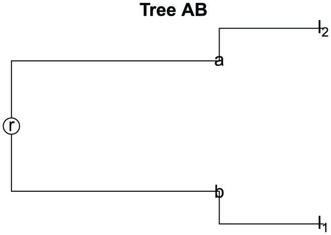
Tree for samples $A$ and $B$.

$$A_t=B_t=3\mathrm{and}{A}_1=B_1=A_2=B_2=2$$

Therefore,

$$\begin{array}{c}{d}^w(A,B)=d(l_1)\left|\frac{2}{3}-\frac{2}{3}\right|+d(l_2)\left|\frac{2}{3}-\frac{2}{3}\right|\\ =0\end{array}$$

with A ≠ B.

1. Consider the samples

$$\begin{array}{l}A=\{r,a_1,a_2\},B=\{r,b_1,b_2,b_2,b_2\}\\ \mathrm{and}C=\{r,r,c_1,c_1,c_1,c_1,c_1,c_1,c_2,c_2\}\end{array}$$

and the trees $T_{AB}$, $T_{AC}$, and $T_{CB}$ built for samples $A$ and $B$, $A$ and $C$, and $C$ and $B$, respectively (see Figure 5), where

Figure 5.

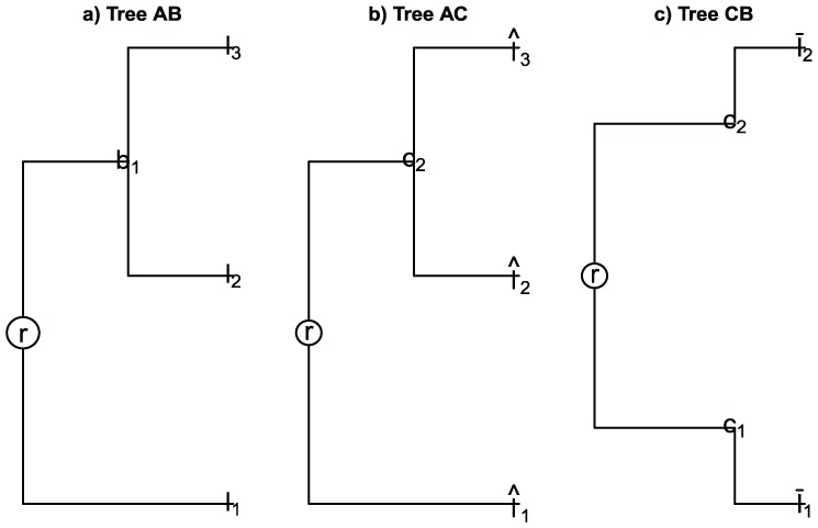
(a) Tree for samples $A$ and $B$. (b) Tree for samples $A$ and $C$. (c) Tree for samples $C$ and $B$.

$$l_2={\widehat{l}}_2=a_1,l_3={\widehat{l}}_3=a_2,l_1={\overline{l}}_1=b_2,{\overline{l}}_2=b_1\mathrm{and}{\widehat{l}}_1=c_1$$ (8)

and also, we assume

$$d(l_2)=d(l_3)$$ (9)

$$d(l_1)>d({\widehat{l}}_1)$$ (10)

From equations (8) and (9), we have that

$$d({\widehat{l}}_2)=d({\widehat{l}}_3)=d(l_2)=d(l_3)$$

If we estimate $d^w(A,B)$, $d^w(A,C)$, and $d^w(C,B)$, we have the following:

$$\begin{array}{c}{d}^w(A,B)=d(l_1)\left|\frac{1}{3}-\frac{4}{5}\right|+d(l_2)\left|\frac{2}{3}-\frac{2}{5}\right|\\ +d(l_3)\left|\frac{2}{3}-\frac{2}{5}\right|\\ =d(l_1)\frac{7}{15}+d(l_2)\frac{8}{15}\end{array}$$ (11)

$$\begin{array}{c}{d}^w(A,C)=d({\widehat{l}}_1)\left|\frac{1}{3}-\frac{4}{5}\right|+d({\widehat{l}}_2)\left|\frac{2}{3}-\frac{2}{5}\right|\\ +d({\widehat{l}}_3)\left|\frac{2}{3}-\frac{2}{5}\right|\\ =d({\widehat{l}}_1)\frac{7}{15}+d({\widehat{l}}_2)\frac{8}{15}\end{array}$$ (12)

$$\begin{array}{l}{d}^w(C,B)=d({\overline{l}}_1)\left|\frac{4}{5}-\frac{4}{5}\right|\hfill \\ +d({\overline{l}}_2)\left|\frac{2}{5}-\frac{2}{5}\right|=0\hfill \end{array}$$ (13)

If the triangle inequality is satisfied, using equalities (11) to (13), we have

$$d(l_1)\frac{7}{15}+d(l_2)\frac{8}{15}\le d({\widehat{l}}_1)\frac{7}{15}+d({\widehat{l}}_2)\frac{8}{15}+0$$

where we can get

$$d(l_1)<\_d({\widehat{l}}_1)$$

this contradicts the supposition (10), so the weighted UniFrac does not comply with the triangle inequality.

We proved that weighted UniFrac satisfies Definition 1; however, it is not a metric.

Normalized weighted UniFrac

The normalized weighted UniFrac was proposed by Lozupone et al² and it is given by

$$d_n^w(A,B)=\frac{{\sum }_{i=1}^{n}d(l_i)|P_i^A-P_i^B|}{D}$$ (14)

where the normalizing factor is

$$D=\sum _{j=1}^{m}d(j)\left(Q_j^A+Q_j^B\right)$$ (15)

with $m$ the number of different sequences in $A\cup B$ and $d(j)$ the distance from the root to the sequence $j\in (A\cup B)$; furthermore,

$$Q_j^A=\frac{{\alpha }_j}{A_t}\mathrm{and}{Q}_j^B=\frac{{\beta }_j}{B_t}$$ (16)

where ${\alpha }_j$ and ${\beta }_j$ are the number of times that the sequence $j$ is observed in samples $A$ and $B$, respectively.

Example 3

In Example 1, $A\cup B=\{a_1,a_2,b_1,b_2\}$, where the sequences proportions in sample $A$ are

$$Q_{a_1}^A=\frac{2}{4},Q_{a_2}^A=\frac{1}{4},Q_{b_1}^A=0,Q_{b_2}^A=0$$

and the sequences proportions in sample $B$ are

$$Q_{a_1}^B=0,Q_{a_2}^B=0,Q_{b_1}^A=\frac{1}{3},Q_{b_2}^B=\frac{1}{3}$$

The normalized weighted UniFrac is less sensitive to branches with a long length and is determined by branches with different proportions.

Proposition 3

The normalized weighted UniFrac is a pseudosemimetric.

Proof

We will prove that the normalized weighted diversity measure UniFrac satisfies Definition 1.

• 1. Analogous to 2. of Proposition 2, we have

$$d_n^w(A,B)=0$$

• 2. To prove symmetry, we consider

$$\begin{array}{c}{d}_n^w(A,B)=\frac{{\sum }_{i=1}^{n}d(l_i)|P_i^A-P_i^B|}{{\sum }_{j=1}^{m}d(j)(Q_j^A+Q_j^B)}\\ =\frac{{\sum }_{i=1}^{n}d(l_i)|P_i^B-P_i^A|}{{\sum }_{j=1}^{m}d(j)(Q_j^B+Q_j^A)}\\ =d_n^w(B,A)\end{array}$$

Thus, the normalized weighted diversity measure UniFrac satisfies with Definition 1. Now, examples where it does not satisfy:

• 1. We consider the example in item (1) from Proposition 2. Therefore,

$$d_n^w(A,B)=0$$

• 2. Consider the samples

$$\begin{array}{l}A=\{r,a_1,a_2\},B=\{r,b_1,b_1,b_1,b_2\}\\ \mathrm{and}C=\{r,r,c_1,c_1,c_1,c_1,c_1,c_1,c_2,c_2\}\end{array}$$

and the trees $T_{AB}$, $T_{AC}$, and T_CB built for samples $A$ and $B$, $A$ and $C$, and $C$ and $B$, respectively (see Figure 6), where

Figure 6.

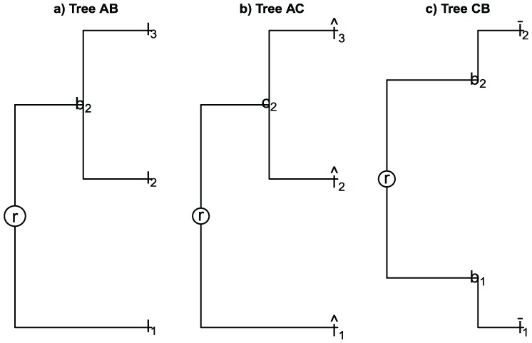
(a) Tree by samples $A$ and $B$. (b) Tree by samples $A$ and $C$. (c) Tree by samples $C$ and $B$.

$$l_1=b_1,l_2={\widehat{l}}_2=a_1,l_3={\widehat{l}}_3=a_2,{\overline{l}}_1={\widehat{l}}_1=c_1,\mathrm{and}{\overline{l}}_2=c_2$$ (17)

and additionally assume

$$d(l_3)=d(l_2)$$ (18)

$$d(l_1)=d(b_2)$$

$$d({\overline{l}}_2)=d({\overline{l}}_1)$$

$$d(l_1)<d({\widehat{l}}_1)$$ (19)

Note that equations (17) and (18) imply that

$$d(l_3)=d(l_2)=d({\widehat{l}}_2)=d({\widehat{l}}_3)$$

Thus,

$$\begin{array}{l}{d}_n^w(A,B)\\ =\frac{d(l_1)|\frac{1}{3}-\frac{4}{5}|+d(l_2)d(l_3)|\frac{2}{3}-\frac{2}{5}||\frac{2}{3}-\frac{2}{5}|}{d(l_1)\frac{3}{5}+d(b_2)\frac{1}{5}+d(l_3)\frac{1}{3}+d(l_2)\frac{1}{3}}\\ =\frac{d(l_1)\frac{7}{15}+d(l_2)\frac{8}{15}}{d(l_1)\frac{4}{5}+d(l_2)\frac{2}{3}}\end{array}$$ (20)

$$\begin{array}{l}{d}_n^w(A,C)\\ =\frac{d({\widehat{l}}_1)|\frac{1}{3}-\frac{4}{5}|+d({\widehat{l}}_2)|\frac{2}{3}-\frac{2}{5}|+d({\widehat{l}}_3)|\frac{2}{3}-\frac{2}{5}|}{d(c_2)\frac{1}{5}+d({\widehat{l}}_1)\frac{3}{5}+d({\widehat{l}}_2)\frac{1}{3}+d({\widehat{l}}_3)\frac{1}{3}}\\ =\frac{d({\widehat{l}}_1)\frac{7}{15}+d({\widehat{l}}_2)\frac{8}{15}}{d({\widehat{l}}_1)\frac{4}{5}+d({\widehat{l}}_2)\frac{2}{3}}\end{array}$$ (21)

$$\begin{array}{l}{d}_n^w(C,B)\\ =\frac{d({\overline{l}}_1)|\frac{4}{5}-\frac{4}{5}|+d({\overline{l}}_2)|\frac{2}{5}-\frac{2}{5}|}{\tilde{D}}=0\end{array}$$ (22)

with $\tilde{D}$ the respective normalizing factor. As the triangle inequality is satisfied using the equalities (20)-(22), we have

$$\frac{d(l_1)\frac{7}{15}+d(l_2)\frac{8}{15}}{d(l_1)\frac{4}{5}+d(l_2)\frac{2}{3}}\le \frac{d({\widehat{l}}_1)\frac{7}{15}+d({\widehat{l}}_2)\frac{8}{15}}{d({\widehat{l}}_1)\frac{4}{5}+d({\widehat{l}}_2)\frac{2}{3}}+0$$

from we can get

$$d({\widehat{l}}_1)<\_d(l_1)$$

it contradict the supposition (10). Therefore, the normalized weighted diversity measure UniFrac does not satisfy the triangle inequality.

We proved that normalized weighted diversity measure UniFrac is a pseudosemimetric. Next, we will give examples where we calculated the diversity measures UniFrac on a tree illustrate by McClelland and Koslicki¹⁶ and we will compare with EMDUniFrac.

EMDUniFrac

Based on Evans and Matsen,¹⁰ the EMDUniFrac is proposed in McClelland and Koslicki,¹⁶ Given two samples $A$ and $B$ of genetic material and their associated abundances, we can estimate two probability distributions $P$ and $Q$ on their phylogenetic tree $T$ that represent the fraction of a given sample that appears at each node in $T$. Let $D$ be the matrix of all pairwise distances between nodes in $T$ and $\Gamma (P,Q)$ describe the space of all ways in which one community can be transformed into the other. The $(i,j)th$ entry of $M\in \Gamma (P,Q)$ indicates the total abundance of $M_{i,j}$ has been moved from node $i$ in sample $P$ to node $j$ in sample $Q$. In this way, the EMDUniFrac is given by

$$EMDUniFrac(P,Q)=\underset{M\in \Gamma (P,Q)}{\min }\sum _{i,j\in T}{D}_{i,j}{M}_{i,j}$$

it represents the minimum amount of ‘work’ required to transform the distribution $P$ into the distribution $Q$ along the phylogenetic tree. It has been previously show that EMDUniFrac(P, Q) is equivalent to weighted UniFrac distance when the sample size is large enough.¹⁰ However, we will give examples where the EMDUniFrac distance and the diversity measures UniFrac are different between them.

Considerate the tree $T$ as in Figure 1(b) in McClelland and Koslicki¹⁶ where EMDUniFrac(P, Q) is $0.2333$. We calculate the diversity measure UniFrac on $T$:

$$\begin{array}{c}{d}^u(A,B)=\frac{d(l_1)(1)+d(l_2)(1)+d(l_3)(0)+d(l_4)(1)}{\frac{6}{5}}\\ =\frac{\frac{3}{10}(3)}{\frac{6}{5}}=\frac{3}{4}=0.75\end{array}$$

Thus,

$$EMDUniFrac(P,Q)=/d^u(A,B)$$

both under $T$.

It is important to mention the samples size is very small.

The weighted diversity measure UniFrac (see expression 7) on the tree $T$ is

$$\begin{array}{l}{d}^w(A,B)=d(l_1)|P_1^A-P_1^B|+d(l_2)|P_2^A-P_2^B|\hfill \\ +d(l_3)|P_3^A-P_3^B|+d(l_4)|P_4^A-P_4^B|\hfill \\ =\frac{3}{10}|0-\frac{1}{3}|+\frac{3}{10}|\frac{1}{2}-0|+\frac{3}{10}|\frac{1}{2}-\frac{1}{3}|\hfill \\ +\frac{3}{10}|0-\frac{2}{3}|\hfill \\ =\frac{3}{10}\left(\frac{1}{3}+\frac{1}{2}+\frac{1}{6}+\frac{2}{3}\right)=\frac{1}{2}=0.5\hfill \end{array}$$

thus, can see that

$$EMDUniFrac(P,Q)=/d^w(A,B)$$

Now, we obtain the normalized weighted UniFrac value as

$$\begin{array}{l}{d}_n^w(A,B)\\ =\frac{\frac{1}{2}}{d(1)\frac{1}{3}+d(2)\frac{1}{2}+d(3)\frac{1}{2}+d(4)\frac{1}{3}+d(5)(0)+d(6)\frac{1}{3}}\\ =\frac{\frac{1}{2}}{\frac{3}{10}\frac{1}{3}+\frac{3}{10}\frac{1}{2}+\frac{3}{10}\frac{1}{2}+\frac{3}{10}\frac{1}{3}+\frac{1}{5}(0)+\frac{1}{5}\frac{1}{3}}\\ =\frac{\frac{1}{2}}{\frac{1}{10}+\frac{3}{20}+\frac{3}{20}+\frac{1}{10}+\frac{1}{15}}=\frac{\frac{1}{2}}{\frac{1}{2}+\frac{1}{15}}=\frac{15}{17}=0.8823\end{array}$$

Thus,

$$EMDUniFrac(P,Q)=/d_n^w(A,B)$$

Therefore, the diversity measures UniFrac and EMDUniFrac are different between them. Then, we can say the diversity measures UniFrac are not equal to EMDUniFrac(P, Q) if the samples size is not large enough.

On the other hand, considerate the tree $T$ as the Figure 1(b) in McClelland and Koslicki,¹⁶ it is built for the different samples $A=\{3,4,5,7\}$ and $B=\{1,2,6,7\}$, we calculate the weighted UniFrac measure as $T$:

$$\begin{array}{l}{d}^w(A,B)=d(l_1)|P_1^A-P_1^B|+d(l_2)|P_2^A-P_2^B|\hfill \\ +d(l_3)|P_3^A-P_3^B|+d(l_4)|P_4^A-P_4^B|\hfill \\ =\frac{3}{10}|\frac{2}{4}-\frac{2}{4}|+\frac{3}{10}|\frac{2}{4}-\frac{2}{4}|+\frac{3}{10}|\frac{2}{4}-\frac{2}{4}|\hfill \\ +\frac{3}{10}|\frac{2}{4}-\frac{2}{4}|\hfill \\ =\frac{3}{10}(0)=0\hfill \end{array}$$

however, samples $A$ and $B$ are different. So that if $A=/B$, it does not imply that $d^w(A,B)=/0$.

Conclusions

In this article, we prove that diversity measures UniFrac, weighted UniFrac, normalized weighted UniFrac satisfy the positive property, symmetry property, and the implication that if the samples are equal then the diversity measures are zero. On the other hand, examples were presented where the diversity measures mentioned do not comply the metric definition. We prove that diversity measures comply the pseudosemimetric definition.

Although measures UniFrac are used in microbiology as a tool to measure the proximity between samples of genetic material large enough and showing a good performance, as mentioned in the literature,^3–7 when the sample size is small, no it is appropriate to use it in that sense. The previous thing due to the lack of the properties previously amended, as Schloss said. In section “EMDUniFrac,” we could see examples where the diversity measures UniFrac and EMDUniFrac are different between them; in this way, we can say the diversity measures UniFrac are not equivalent to EMDUniFrac if the samples size is not large enough. Furthermore, if we calculate the weighted UniFrac for two different small samples, it does not imply that weighted UniFrac is zero. Then an alternative for diversity measures UniFrac is the Kantorovich-Rubinstein metric¹⁰ or EMDUniFrac metric.^18–20

References

- 1. Lozupone CA, Knight R. UniFrac: a new phylogenetic method for comparing microbial communities. Appl Environ Microbiol. 2005;71:8228–8235. [DOI] [PMC free article] [PubMed] [Google Scholar]
- 2. Lozupone CA, Hamady M, Kelley ST, Knight R. Quantitative and qualitative β diversity measures lead to different insights into factors that structure microbial communities. Appl Environ Microbiol. 2007;73:1576–1585. [DOI] [PMC free article] [PubMed] [Google Scholar]
- 3. Frank DN, Amand ALS, Feldman RA, Boedeker EC, Harpaz N, Pace NR. Molecular-phylogenetic characterization of microbial community imbalances in human inflammatory bowel diseases. Proc Natl Acad Sci U S A. 2007;104:13780–13785. [DOI] [PMC free article] [PubMed] [Google Scholar]
- 4. Costello EK, Lauber CL, Hamady M, Fierer N, Gordon JI, Knight R. Bacterial community variation in human body habitats across space and time. Science. 2009;326:1694–1697. [DOI] [PMC free article] [PubMed] [Google Scholar]
- 5. Charlson ES, Bittinger K, Haas AR, et al. Topographical continuity of bacterial populations in the healthy human respiratory tract. Am J Respir Crit Care Med. 2011;184:957–963. [DOI] [PMC free article] [PubMed] [Google Scholar]
- 6. Ley RE, Bäckhed F, Turnbaugh P, Lozupone CA, Knight RD, Gordon JI. Obesity alters gut microbial ecology. Proc Natl Acad Sci U S A. 2005;102:11070–11075. [DOI] [PMC free article] [PubMed] [Google Scholar]
- 7. Chang Q, Luan Y, Sun F. Variance adjusted weighted UniFrac: a powerful beta diversity measure for comparing communities based on phylogeny. BMC Bioinformatics. 2011;12:118. [DOI] [PMC free article] [PubMed] [Google Scholar]
- 8. Chen J, Bittinger K, Charlson ES, et al. Associating microbiome composition with environmental covariates using generalized UniFrac distances. Bioinformatics. 2012;28:2106–2113. [DOI] [PMC free article] [PubMed] [Google Scholar]
- 9. Schloss PD. Evaluating different approaches that test whether microbial communities have the same structure. ISME J. 2008;2:265. [DOI] [PubMed] [Google Scholar]
- 10. Evans SN, Matsen FA. The phylogenetic Kantorovich-Rubinstein metric for environmental sequence samples. J R Stat Soc Series B Stat Methodol. 2012;74:569–592. [DOI] [PMC free article] [PubMed] [Google Scholar]
- 11. Rachev ST. Probability Metrics and the Stability of Stochastic Models, Volume 269. Hoboken, NJ: John Wiley & Son Ltd; 1991. [Google Scholar]
- 12. Rachev ST, Rüschendorf L. Mass Transportation Problems, Volume I: Probability and Its Applications. New York, NY: Springer; 1998. [Google Scholar]
- 13. Villani C. Topics in Optimal Transportation. Providence, RI: American Mathematical Society; 2003. [Google Scholar]
- 14. Villani C. Optimal Transport: Old and New. Grundlehren der mathematischen Wissenschaften. Berlin, Germany: Springer; 2008. [Google Scholar]
- 15. Levina E, Bickel P. The earth mover’s distance is the mallows distance: some insights from statistics. In: Proceedings Eighth IEEE International Conference on Computer Vision. ICCV 2001, vol. 2 New York, NY: IEEE; 2001:251–256. [Google Scholar]
- 16. McClelland J, Koslicki D. EMDUnifrac: exact linear time computation of the Unifrac metric and identification of differentially abundant organisms. J Math Biol. 2018;77:935–949. [DOI] [PubMed] [Google Scholar]
- 17. Warnow T. Computational Phylogenetics. An Introduction to Designing Methods for Phylogeny Estimation. Cambridge, UK: Cambridge University Press; 2017. [Google Scholar]
- 18. Srinivasan S, Hoffman NG, Morgan MT, et al. Bacterial communities in women with bacterial vaginosis: high resolution phylogenetic analyses reveal relationships of microbiota to clinical criteria. PLoS ONE. 2012;7:e37818. [DOI] [PMC free article] [PubMed] [Google Scholar]
- 19. Smith BC, McAndrew T, Chen Z, et al. The cervical microbiome over 7 years and a comparison of methodologies for its characterization. PLoS ONE. 2012;7:e40425. [DOI] [PMC free article] [PubMed] [Google Scholar]
- 20. Livermore JA, Mattes TE. Phylogenetic detention of novel cryptomycota in an Iowa (United States) aquifer and from previously collected marine and freshwater targeted high-throughput sequencing sets. Environ Microbiol. 2013;15:2333–2341. [DOI] [PubMed] [Google Scholar]