Simplifying the Implementation of Modern Scale Scoring Methods with an Automated R Package: Automated Moderated Nonlinear Factor Analysis (aMNLFA)

Abstract

When generating scores to represent latent constructs, analysts have a choice between applying psychometric approaches that are principled but that can be complicated and time-intensive versus applying simple and fast, but less precise approaches, such as sum or mean scoring. We explain the reasons for preferring modern psychometric approaches: namely, use of unequal item weights and severity parameters, the ability to account for local dependence and differential item functioning, and the use of covariate information to more efficiently estimate factor scores. We describe moderated nonlinear factor analysis (MNLFA), a relatively new, highly flexible approach that allows analysts to develop precise factor score estimates that address limitations of sum score, mean score, and traditional factor analytic approaches to scoring. We then outline the steps involved in using the MNLFA scoring approach and discuss the circumstances in which this approach is preferred. To overcome the difficulty of implementing MNLFA models in practice, we developed an R package, aMNLFA, that automates much of the rule-based scoring process. We illustrate the use of aMNLFA with an empirical example of scoring alcohol involvement in a longitudinal study of 6,998 adolescents and compare performance of MNLFA scores with traditional factor analysis and sum scores based on the same set of 12 items. MNLFA scores retain more meaningful variation than other approaches. We conclude with practical guidelines for scoring.

Latent constructs are common in the field of addiction research. Constructs like “addiction severity” or “risky adolescent drinking” cannot be measured with a single item; instead, we must use several items to capture an underlying latent construct. There are more and less precise approaches for achieving this goal. On the less precise end of the continuum, we can sum or average items. On the more precise end of the continuum, we can use modern psychometric approaches like item response theory (IRT) or factor analysis to account for the relationship of each item to the underlying latent construct and for differential item functioning (DIF) across groups (e.g., gender, age) when constructing scores (e.g., Lindhiem, Bennett, Hipwell, et al., 2015).

With increased precision comes increased effort and the need for specialized knowledge and possibly expensive software. These barriers may discourage adoption of superior psychometric techniques for scoring. We have reduced this barrier by developing an R package that automates many of the steps involved in conducting modern psychometric analysis using the moderated nonlinear factor analysis model (MNLFA), a method that encompasses and expands upon traditional factor analysis and IRT (Bauer & Hussong, 2009; Bauer, 2017). The outline of this manuscript is as follows. First, we explain why simple approaches to scoring, like sum scores, can lead to undesirable results: the assumptions of equal item weighting and unidimensionality and inattention to item severity. Then we discuss the consequences of using a traditional factor analytic scoring method in the presence of DIF, and we introduce properties of IRT and factor analysis that address these problems. We then describe MNLFA, a flexible model that generalizes these approaches (Bauer, 2017). We outline the steps involved in conducting MNLFA and introduce our automated R package, aMNLFA. Finally, we illustrate the use of aMNLFA in an empirical example and we compare the performance of scores obtained using aMNLFA versus traditional factor analysis and sum scores.

Problems with Traditional Scoring Methods

Despite their ease of implementation, simple scoring methods require four problematic assumptions that we describe in this section.

Equal item weights.

When items are summed or averaged, each item contributes equally to the overall score (assuming all items have equivalent response scales). There are undesirable consequences of this approach. For example, when measuring depressive symptoms with the CES-D, an endorsement of having trouble sleeping would have equal weight to having thoughts of suicide—both items would be given a weight of “1” for a sum score or a weight that is inversely proportional to the number of items for a mean score. To make matters worse, if items are not scaled identically (e.g., see Table 1), then it is not obvious how best to compute sum or mean scores since equal weights are not face valid. Similarly, it is not obvious how to handle item-level missing data when computing sum or mean scores.

Table 1.

Items used to measure alcohol involvement

Variable		Responses
Label	Question	Options*
AU2	During the last 3 months, about how many days did you have 1 or more drink of alcohol?	0,1–2,3–5,6+
AU3	About how much did you usually have when you drank in the last 3 months?	<1, 1, 2, 3, or 4+
During the past 3 months, about how many times have you …
AU4	Had 3 or 4 drinks in a row?	0 ,1–2, 3–5, 6+
AU5	Had 5 or more drinks in a row?	0, 1–2, 3+
AU6	Gotten drunk or very high from drinking alcoholic beverages?	0, 1–2, 3–5, 6+
AC7	Drunk alcohol when you were alone?	0, 1–2, 3+
AU8	Been hung over?	0, 1–2, 3+
AC1	Gotten in trouble with your parents because you had been drinking?	0, 1–2, 3+
AC2	Had problems with someone you were dating because you had been drinking?	0, 1–2, 3+
AC3	Did something you later regretted because you had been drinking?	0, 1–2, 3+
AC4	Gotten into a sexual situation that you later regretted because you	0, 1+
	had been drinking?
AC5	Gotten into a physical fight because you had been drinking?	0, 1+

^*Response options were collapsed in some cases to avoid cell sparseness

While the assumption of equal item weights is necessary in simple scoring methods, it is not required with modern methods like factor analysis or IRT. With these more complex methods, it is assumed that one or more latent constructs underlie item responses. Items that are more strongly correlated with other items on the scale are given more weight and items that contain more unique variance are given less weight. In the depression example, suicidal ideation, which may be more specific to depression and correlate highly with other items, would receive greater weight in scoring the latent depression construct whereas trouble sleeping, which may be less specific to depression and relate to many factors such as caffeine intake, room temperature, and spousal snoring, would receive less weight in scoring the latent depression construct.

Unidimensionality.

There are two issues related to unidimensionality that arise when using sum or mean scores to measure latent constructs, both of which can be addressed using modern psychometric scoring approaches. The first is that the set of items used to generate an individual’s score on a construct may not actually reflect a single latent construct, but these simpler scoring approaches assume that they do. For instance, items used to measure social motivations for alcohol use might tap several distinct dimensions (e.g., sociability, general motivation to drink, social anxiety). Failure to establish a unidimensional factor structure results in misleading scores.

Another issue related to dimensionality, but which can occur for items that do tap a single construct, is the problem of local dependence. Local dependence arises when two or more items are redundant, or when they are correlated for reasons other than the latent construct. For instance, negatively-worded items may be more correlated with one another than they are with positively-worded items, or items sharing the same question prompt may be correlated as an artefact of the prompt (e.g., “How much do you agree or disagree with each of the following statements?”). If ignored, local dependence results in invalid and biased measurement because the meaning of the latent construct shifts toward the cause of local dependence (Hambleton, Swaminathan, & Rogers, 1991). It is not possible to test for local dependence with simple scoring methods, but psychometric approaches like factor analysis and IRT make it straightforward to identify and address local dependence. When the number of items is large, one item in a pair of locally dependent items can be dropped. When dropping items is undesirable, residual correlations can be incorporated into the model.

Assumption of equal severity.

Some items are more “difficult” to endorse, or are more “severe,” than are others. Endorsement of more severe items should increase a person’s score more than endorsement of less severe items because these items distinguish amongst individuals at higher levels of the latent factor. For instance, an item assessing whether an adolescent experienced a blackout from a drinking episode might be more severe than an item assessing whether the adolescent had ever gotten in trouble with their parents as a result of drinking. The concept of severity is not present in simpler scoring methods, whereas modern psychometric methods account for it.

Differential item functioning.

A final limitation of simple scoring methods is that they cannot accommodate DIF. DIF occurs when the weight or severity of an item depends on a characteristic of the individuals being scored that is unrelated to the latent construct of interest, like race, gender, age, or socioeconomic status. For example, girls tend to endorse crying more frequently than boys on depression scales, regardless of their actual level of depression (Steinberg & Thissen, 2006). When group differences in measurement properties are ignored during scoring, they masquerade as true group differences on the latent construct when they are simply artefacts of measurement (Millsap, 1998). This can cause serious errors in inference, clinical assessment, and could even lead to misguided public policy.

DIF can also occur with ordinal items when the distance between response options varies as a function of an individual or group-level characteristic. This is particularly likely to arise when harmonizing across studies that use similar measures, but different response options. For instance, one study might ask: “How often did you use alcohol in the past 3 months,” giving options “never,” “sometimes,” or “frequently,” and another study might ask the same question, but provide participants with options “never,” “1–4 times a week,” “5–7 times a week.” In this example, we would not expect for the item loadings or severity to differ across the studies, but the thresholds for the level of alcohol use required in order to select each of the three options might vary across studies.

In sum, simple scoring methods make strong assumptions, the violation of which can lead to serious errors of inference. The first three of the four limitations described in this section are addressed by standard psychometric models like factor analysis and IRT. The general goal of these techniques is to model the relationships between multiple indicators and latent variables, and not to incorporate information about individual differences into measurement. However, traditional psychometric approaches are limited in how well they can address the fourth concern and can only handle measurement differences across a very small number of discrete groups (e.g., male vs. female or Black vs. White). In the following section, we provide a brief overview of traditional factor analysis before introducing MNLFA, an approach that can address all four of the limitations laid out in this section.

Traditional Factor Analysis

Factor analysis and IRT are very similar methods and are equivalent under many scenarios (Takane & De Leeuw, 1987; Wirth & Edwards, 2007). Historically, factor analysis was used with continuous items or scales and IRT was used for discrete response distributions; however, factor analysis is no longer constrained for use with continuous response distributions.¹ In this section, we provide a background on the basic underpinnings of traditional factor analysis models because they provide a notation that is more easily extended to introduce MNLFA than that used in the IRT tradition.

The traditional factor analysis model, represented graphically on the left side of Figure 1, assumes that correlations between items (represented as rectangles labeled “y₁” through “y₄”) arise from a common factor or factors (η) that in turn give rise to item responses. In factor analysis, each factor represents a unidimensional construct. Although only one factor is depicted in Figure 1, it is possible to model multiple common factors. Additionally, local dependence between items can be accommodated by permitting residual correlations between dependent items – these correlations allow items to be more correlated with one another than would be expected given their association with the common factor(s). An example of a residual correlation is depicted between y₁ and y₂ in the figure. Items are differentially related to η, as represented by the unique item weights, λ (also called “factor loadings”). Finally, each item has its own intercept, τ, which represents its level of difficulty or severity.²

Figure 1.

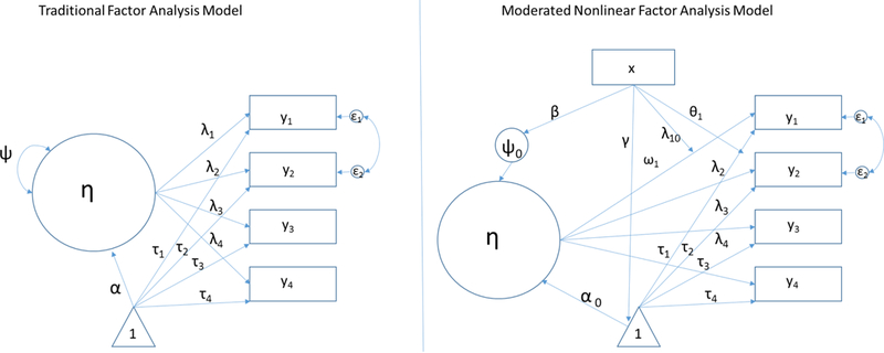
Path diagrams representing a traditional factor analysis model (left; i.e., confirmatory factor analysis) and a moderated nonlinear factor analysis (MNLFA) model (right). Paths represented in these figures have a one-to-one correspondence with equations in the text.

Moderated Nonlinear Factor Analysis (MNLFA)

MNLFA extends the flexibility of traditional psychometric models in a few ways (Bauer, 2017). First, traditional psychometric models like IRT and factor analysis require the use of multiple groups models to account for DIF. As such, it is only feasible to accommodate DIF for a few discrete groups before the models become unwieldly, under-powered, and difficult to interpret. If measurement is expected to vary as a function of a continuous variable, such as age, then it is necessary to dichotomize or trichotomize the continuous variable for use in the multiple groups framework. In contrast, MNLFA incorporates estimation of more complex patterns of DIF using item weights (i.e., factor loadings) and severity parameters (i.e., item intercepts) that are regressed on any number of discrete or continuous predictors, their interactions, and polynomial expansions of these predictors (e.g., age²). Similarly, latent variable means and variances can be regressed on these predictors to increase measurement precision (Thissen & Wainer, 2001). The latter parameters are referred to as “impact” parameters (i.e., mean impact and variance impact). In the depression example, we might expect age to have mean and variance impact in a sample of adolescents because depression symptoms tend to increase over pubertal development and we might see more inter-individual variation among older adolescents. Thus, impact reflects true differences on the latent construct, whereas DIF represents a measurement artefact.

Mathematical details of MNLFA are available elsewhere (Bauer, 2017; Bauer & Hussong, 2009; Curran, McGinley, Bauer, et al., 2014). We provide only a brief overview here, linking the equations with the path diagram on the right side of Figure 1.

In MNLFA, factor scores for an individual i, denoted α_i, are a function of an overall intercept,α₀, plus a weighted linear combination of K predictors. Figure 1 shows a single predictor, x. However, there are few constraints on the set of predictors that can be used. As mentioned above, predictors can take any distributional form and can include polynomial terms or interactions. Factor variances, denoted &ψ_i, are conditional on an intercept, ψ₀, multiplied by an exponential function of K predictors. An exponential function is used to avoid negative variances. Thus, the mean and variance impact equations take the following form:

$$\begin{gathered} {\alpha }_i={\alpha }_0+\sum _K{\gamma }_k{x}_{ki} \\ {\psi }_i={\psi }_0{e}^{\sum _K{\beta }_k{x}_{ki}}. \end{gathered}$$ (1)

Similarly, the item weights (i.e., factor loadings, λ_ti ) are each a function of an overall mean loading, λ_0t plus a linear combination of K predictors. Item severity parameters (i.e., intercepts, τ_ti ) are a function of an overall mean severity parameter, τ_0t plus a weighted combination of K predictors. The DIF equations take the following form:

$$\begin{gathered} {\lambda }_{ti}={\lambda }_{0t}+\sum _K{\theta }_{tk}{x}_k \\ {\tau }_{ti}={\tau }_{0t}+\sum _K{\omega }_{tk}{x}_k. \end{gathered}$$ (2)

Although we index K predictors for each of the MNLFA equations, it is not necessary to use the same K predictors across all equations within a given model. It is only necessary that predictors that are included in the factor loading equations are also included in the item intercept equations. The reason is equivalent to the reason why it is necessary to include main effects of a variable whenever it is used in an interaction term (i.e., $E[y_{ti}]={\tau }_{ti}+{\lambda }_{ti}{\eta }_i$ ).

Curran and colleagues (2014) outlined a recommended procedure for conducting MNLFA that we summarize and expand here.

1. Establish unidimensional construct(s). Although it is possible to fit a multifactor MNLFA for multidimensional scales, it is more computationally efficient to run separate one-factor models for each unidimensional item set. Therefore, we recommend identifying unidimensional factors that can be handled separately in MNLFA for the purpose of assessing impact and DIF. If desired, one can follow up these analyses by fitting a single, multidimensional MNLFA that incorporates the impact and DIF determined from the separate unidimensional models (see Bauer, 2017, for an example).

2. Data visualization to identify potential DIF or impact. Inspect item frequencies, collapsing sparse categories as necessary. Plot item responses as a function of the K predictors for which DIF or impact is suspected. If data are longitudinal, items responses can be plotted over time as a function of other predictors, like gender. These plots help researchers to predict effects they can expect to encounter in the MNLFA. The analyst will notice that some predictor effects appear to be constant across items: this type of pattern represents impact. Other predictor effects will be exclusive to certain items. This pattern is consistent with DIF.

3. Draw a calibration sample. This step applies only when data are nested or longitudinal. The purpose is to draw a sample of independent observations by choosing one observation per cluster. Subsequent steps will be conducted with the calibration sample until the scoring step (step 8), when the full sample is again used. One may wish to repeat these analyses with a second randomly drawn calibration sample to determine model stability.

4. Initial impact assessment. Regress factor means and variances on the same K predictors investigated in step 2, including any hypothesized interactions or polynomial terms (e.g., age²). However, for computational feasibility, we recommend against including interaction terms or polynomial effects in variance impact equations unless there is a clear rationale for doing so. Because predictor effects will be trimmed in subsequent steps, we recommend using alpha = .10 to retain impact effects in this step.

5. Initial DIF assessment. In line with the IRT LR-DIF approach of assuming invariance of all other items while testing DIF in one measure at a time (Finch, 2005; Woods, 2011), test predictor effects on factor loadings and item thresholds for one item at a time, allowing all other items to serve as non-invariant “anchors” for the latent construct. We use an alpha level of .05 for retaining predictor effects on factor loadings in this step. We use a stricter alpha level for DIF effects because multiple testing is a concern (Finch, 2005). As noted previously, any predictor effect that is significantly related to the item’s factor loading must be remain as a predictor for item intercepts, as well as any additional intercept predictors meeting the alpha = .05 criterion.

6. Test all impact and DIF effects simultaneously. The purpose of this step is to form the final scoring model that accounts for DIF and impact effects simultaneously. Computationally, it would not be possible to estimate all possible DIF and impact effects in a single model because the model would not be identified, so all effects that met the preliminary alpha criteria in steps 4 and 5 are included in a single model in this step. By trimming obviously nonsignificant effects in the previous steps, we are in a better position to uncover true effects in this step. Out of concern for Type I error resulting from multiple significance tests for DIF parameters, we sequentially apply the Benjamini-Hochberg family-wise error correction to λ (loading) DIF parameters, and then, because all items with significant factor loading DIF necessarily are permitted to have intercept DIF, the Benjamini-Hochberg correction is applied to all τ (intercept) DIF parameters for items with no significant loading DIF.

7. Obtain parameter estimates for the final scoring model. In this last step with the calibration sample, the set of effects identified in step 6 are included in a final MNLFA in order to obtain parameter estimates for the DIF and impact effects that can be applied to the full sample. Note that if data are not nested, this step can be combined with step 8.

8. Generate scores for the full sample. In this step, the MNLFA parameters are fixed (i.e., not estimated, but held constant at a given value) to the parameter estimates that were obtained with the calibration sample so that these parameters can be used to generate factor score estimates for every case in the full sample without bias.

9. Visual inspection of results. In this step, factor score estimates are plotted against time (if applicable) and other predictors to confirm that patterns of results align with what would be expected given data visualization in step 1. This step can also include inspection of individual items as a function of factor score estimates.

Although we are convinced of the benefits of improved scoring that result from implementation of these models, we have no illusions about the difficulty of implementing this scoring method. We have spent countless hours specifying these models, in the process identifying and correcting errors that have cost us time. It is for these reasons that we developed automated code that would allow us to carry out the full MNLFA procedure outlined above so that each MNLFA analysis takes substantially less user input than would be otherwise required. By using our aMNLFA package, we have cut down on time and errors while retaining the benefits of using a high-quality scoring method (e.g., Gottfredson et al., 2017).

With few exceptions (e.g., Smith, Rose, Mazure, et al., 2014; Witkiewitz, Hallgren, O’Sickey, et al., 2016), MNLFA has not been widely adopted. We hope that by formalizing aMNLFA into a readily-available and documented R package, and by illustrating its use here, other researchers will be able to experience these benefits. We now walk through an illustrative example of how aMNLFA is used to generate factor score estimates. More detailed information about the package and its functionality is available in the online appendix.

Empirical Example

Data for this example are from a longitudinal study of N=6,998 adolescents in grades 6 through 12 for all middle and high schools within three North Carolina counties. The study followed an accelerated cohort-sequential design and surveys were administered during school with written consent from adolescents and a waiver of written parental consent. Surveys were administered every semester for six waves, and the seventh wave was administered one year after the sixth wave. Study protocols were approved by the UNC IRB. 50% of the students were male, 52% of the students identified as White and 37% identified as Black. Additional details of the sample and procedure are provided elsewhere (e.g., Ennett et al., 2006).

For the purposes of this paper we will examine the alcohol involvement construct measured with the 12 indicators summarized in Table 1. We tested impact and DIF as a function of semester in school (Spring of 6^th grade through Fall of 12^th grade), gender, race/ethnicity, maximum level of education ever reported for either parent (high school or less, some college or technical school, college degree or higher), cohort (1, 2, or 3), and high school attended. A traditional psychometric scoring approach would require evaluating differences in measurement properties for each of these groupings separately, which is problematic because many of these factors are collinear. MNLFA allows us to model them simultaneously, including a test of a quadratic effect of grade and linear interactions between grade and other factors. Although items are ordinal and thus have threshold parameters, we chose not to evaluate the possibility of threshold DIF in this example because item response options stayed constant for all waves, so threshold DIF would be unlikely.

We first cleaned the data by collapsing sparse cells in the alcohol items and centering predictors. Grade was centered at the first observed time point, in the spring of 6^th grade. Gender, parental education, and race/ethnicity were effect-coded to allow the intercepts of the item parameters to reflect the mean across all groups. We then conducted exploratory factor analysis to evaluate dimensionality. (See the online appendix for details on data formatting required for aMNLFA.)

Our package contains eight functions necessary to conduct a complete MNLFA using the aMNLFA package. These functions are listed in Table 2 and a video demonstration of their application in this empirical example is available here: https://nishagottfredson.web.unc.edu/amnlfa/; function details are described in depth in the online appendix). In terms of software requirements, R is free to use and can be downloaded here: www.r-project.org/. aMNLFA utilizes the free MplusAutomation package (Hallquist & Wiley, 2017) to generate Mplus input scripts and to read in Mplus output files. Access to Mplus is required to run the input files (www.statmodel.com).

Table 2.

aMNLFA functions in order of application

aMNLFA step	Function name	Purpose	User inputs	Outputs	External actions required
NA	aMNLFA.object	Generate aMNLFA object, which is an object containing all the relevant information about the analysis; this will be referenced throughout the aMNLFA process.	Data in appropriate format (described in the online appendix), file path, list of unidimensional item labels and response type (normal, categorical), time variables, ID variable (if applicable), variables to be included in DIF model, variables to be included in mean and variance impact models, Boolean operator (i.e., TRUE or FALSE) indicating whether to assess threshold DIF.	aMNLFA object in R workspace (with a user- specified name).	None.
2 – Data visualization	aMNLFA.itemplots	Generate item plots as a function of predictors (including time)	aMNLFA object created in step 1	PNG files containing graphs in parent folder. All factor indicators are scaled continuously in these plots.	Open PNG files that are generated by this step to visualize items as a function of predictors.
3 – Draw a calibration sample	aMNLFA.sample	Prepare data. If data are nested by drawing a calibration sample and format for Mplus. Otherwise, simply format for Mplus	aMNLFA object created in step 1	Flat text file called (“sample.dat”) containing prepared data in parent folder.	None.
4 – Initial impact assessment & 5 – Initial DIF assessment	aMNLFA.initial	Generate initial mean and variance impact and item wise DIF models.	aMNLFA object created in step 1	One Mplus input file each for mean impact, variance impact, and DIF for each item, in parent folder.	Use Mplus to open and run the pre-populated input files. These models may take several hours to converge. Limit computational problems by simplifying the variance impact model. Once these models have converged, proceed to the next step.
6 – Test all impact and DIF effects simultaneously	aMNLFA.simultaneous	Run a simultaneous MNLFA model using trimmed results from the previous step	aMNLFA object created in step 1	One Mplus input file for fitting simultaneous MNLFA.	Open Mplus to run the pre-populated input file. This model may take several hours to converge. Once this model has converged, proceed to the next step.
7 – Obtain parameter estimates for the final scoring model skip if data are not nested)	aMNLFA.final	Obtain final parameter estimates	aMNLFA object created in step 1	One Mplus input file for fitting final model.	Open Mplus to run the pre-populated input file. This model make take several hours to converge. Once the model has converged, proceed to the next step.
8 – Generate scores for the full sample	aMNLFA.scores	Generate factor score estimates for the full sample	aMNLFA object created in step 1	One Mplus input file for scoring.	Open Mplus to run the pre-populated input file. Scores will be available in a file called “scores.dat.”
9 – Visual inspection of results	aMNLFA.scoreplots	Visually inspect factor score estimates.	aMNLFA object created in step 1	PNG files containing graphs in parent folder, and merged data file containing scores for entire dataset.	Open PNG files to inspect factor score estimates as a function of predictors.

A sample of item plots resulting from the aMNLFA.plot function are shown in Figure 2. This set of item plots compares mean responses to the 12 alcohol involvement items over time for Black students and for White students. Other racial/ethnic groups are not included here due to small cell sizes. We see that White students tend to use much more alcohol than Black students and that these differences grow over time (AU2 and AU3). A similar, but less extreme, pattern is observed for the more severe items (e.g, AU6). Thus, we might expect to find mean impact as a function of race and an interaction between race and grade, with the potential for significant DIF parameters to capture different magnitudes of racial differences across items.

Figure 2.

A sample of plots generated by the aMNLFA.itemplots function. Items are described on Table 1. Average item response values for alcohol involvement items over time as a function of race/ethnicity. Bubble size is proportional to the sample size contributing to each mean estimate. Grade is mean centered in this plot.

Having first established unidimensionality, we drew a calibration sample using the aMNLFA.sample function; the resultant data file contained one record per subject. We created the Mplus input files using the aMNLFA.initial, aMNLFA.simultaneous, and aMNLFA.final functions, and ran them in order.³ This required little effort except for pointing R to the correct file locations, providing variable names, and monitoring model convergence in Mplus. We note that these are the steps that are typically time-consuming from a data management perspective, and extremely error-prone. By automating this rule-based procedure, the major barrier to implementing MNLFA models has been removed.

As a final step, we used the aMNLFA.scoreplots function to create plots of the factor score estimates as a function of semester in school, gender, parental education, and race. One of the sample plots generated by this step is displayed in Figure 3. Factor score estimates follow the same pattern that we observed from the item plots in Figure 2: White students have higher alcohol involvement scores than Black students and these differences become wider across development. Importantly, the factor score estimates generated using the MNLFA approach are not biased as a result of artefactual measurement differences across Black and White students as they might be had DIF not been taken into account (Millsap, 1998).

Figure 3.

A sample plot produced using the aMNLFA.scoreplots function: alcohol involvement factor score estimates over time as a function of race/ethnicity. Bubble size is proportional to the sample size contributing to each mean estimate. Grade is mean centered in this plot.

The final scoring model showed evidence for positive mean impact (i.e., higher average levels of alcohol involvement) for adolescents whose parents had low levels of education and for grade. We found negative mean impact for Black students and males, a quadratic effect of grade, and a grade-by-race interaction. We also found mean impact for school membership and cohort. Gender exerted variance impact such that alcohol involvement was more variable for males than for females. We found no evidence for factor loading DIF, but race/ethnicity exerted intercept DIF for items AU4 and AU5, meaning that, although White students endorsed these items more overall, Black students were more likely to endorse these items than White students holding the true, underlying level of alcohol involvement constant.

Comparison of Scores

Although the aMNLFA package greatly reduces the effort required to generate scores based on this method, other scoring methods are still easier to implement. To evaluate the utility of using the MNLFA method versus the sum score and traditional factor analysis methods, we compared the performance of these scores. Sum scores were generated by rescaling all items to range from 0 to 1 and then summing the rescaled variables. Items were rescaled to avoid giving excess weight to items with more response options. Traditional factor score estimates were generated using the same set of factor indicators as MNLFA using Mplus, but no DIF or impact effects were included in the confirmatory factor model.

Figure 4 shows univariate and bivariate distributions of sum scores, CFA scores, and MNLFA scores. MNLFA scores are highly correlated with CFA scores (r=.96) and somewhat less with sum scores (r=.84). CFA scores are highly correlated with sum scores (r=.92). Despite the high correlations with MNLFA scores, sum scores and CFA scores are extremely zero-inflated and skewed. In contrast, the MNLFA-based scores are more variable and follow a bimodal distribution. Additionally, because grade exerted strong impact on alcohol involvement, MNLFA scores retained a stronger association with grade than CFA or sum scores: r=.36 for MNLFA scores, r=.21 for CFA scores, and r=.19 for sum scores. Race had smaller impact on alcohol involvement true scores, so the difference between scoring method was not as stark when correlating scores with race (Black versus White): r=−.12 for MNLFA scores, r=−.10 for CFA scores, and r=−.09 for sum scores.

Figure 4.

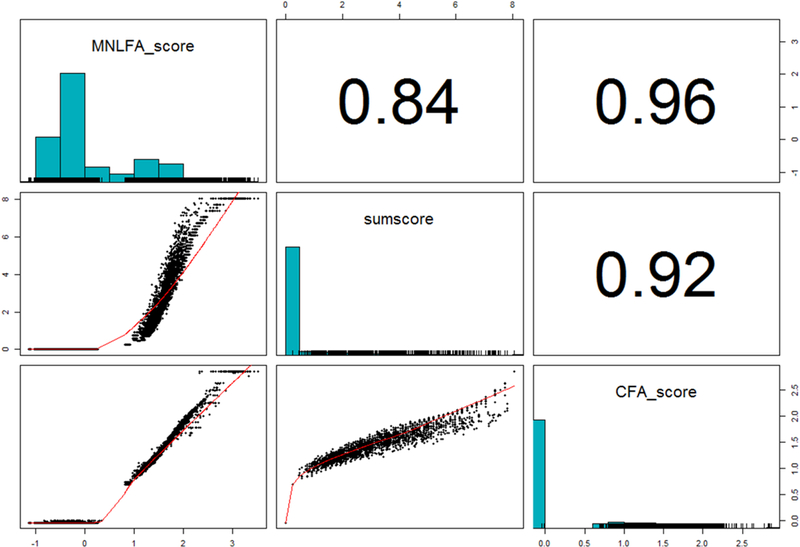
Univariate (on diagonal) and bivariate comparison of scoring techniques. Pearson correlations are in the upper diagonal. MNLFA = moderated nonlinear factor analysis. CFA = confirmatory factor analysis.

Although these results are only from a single dataset, they are in line with those obtained in simulation research that examined a broader set of conditions: CFA and MNLFA scores tend to be similarly rank-ordered with MNLFA scores only slightly more correlated with the underlying true scores (Curran et al., 2018). However, when used in secondary predictive models, CFA scores often produce badly biased estimates whereas this bias is much reduced when using MNLFA scores (Curran et al., 2018). Differences between the scoring methods are starkest when there are relatively few factor indicators.

Discussion

The goal of this special issue is to identify and correct for barriers to the implementation of quantitative advances in the field of addiction research. As methodologists, we are committed to optimizing the precision and validity of scores that we obtain from measures that are collected for study participants and to preventing imprecise or incorrect scientific inferences to the extent possible. MNLFA is a flexible approach that permits regression of factor means, variances, factor loadings, intercepts, and thresholds on covariates that can follow any distributional or functional form.

Limitations and Practical Considerations

In spite of its advantages, there are at least two circumstances when it may not make sense for researchers to implement MNLFA for scoring. The first is when the sample size is small. Use of complex statistical methods with small samples can lead to less stable models that capitalize on chance and do not generalize well in other samples. Simulation studies have found stable results with samples as low as 500 so it is not clear yet what the sample size requirements for MNLFA models are. The answer likely varies depending on model complexity (e.g., number of indicators and covariates), but we have found results to be stable with sample sizes around N=200 when used in practice. The second scenario when MNLFA is not feasible is when researchers do not have access to the software programs needed to run these models. Although the aMNLFA R package is free to use, Mplus is not.

In its current form, aMNLFA does not compute effect sizes and we recommend using simple significance testing to determine which DIF effects to allow in the final model. Future research should draw from IRT literature on DIF effect sizes to generate guidelines for MNLFA users regarding what constitutes meaningful DIF beyond patterns of statistical significance.

Conclusion

As applied addiction researchers, we are attuned to the costs associated with implementing more complex analysis methods when simpler methods are available. It is because of this tension that we designed the aMNLFA package to facilitate implementation of MNLFA. We hope that this package will make it possible for our colleagues to implement more optimal measurement practices in their own work, and ultimately improving the statistical validity of work in addiction science.

Highlights.

• Moderated nonlinear factor analysis generates more precise scores than traditional methods.

• We created an R package (aMNLFA) to facilitate application of this approach.

• Application of the package is illustrated

• Factor scores generated using aMNLFA contained more meaningful variation than sum scores.

Online Appendix: Instructions for Using Automated Moderated Nonlinear Factor Analysis (aMNLFA)

Preparing the data

• ○Column headers must be in all-caps with no periods. Keep names short (8 characters max)
• ○
  Nominal predictors should be hard coded in two formats:

  1. A single variable with all nominal levels included
  2. Contrast-coded variables for all levels except the reference level.
• ○Hard-code interaction terms. Use the first three characters from each main effect with an underscore in between. Example: interaction between ABCDEFG and ZYXWV should be named ABC_ZYX.
• ○Hard-code quadratic terms. Use the first three characters of the linear term followed by _2. Example: GRADE and GRA_2.
• ○If data are longitudinal, the file should be in long format (one record per response occasion) o Read the data in as an R dataframe. This may be done using the read.table function, e.g.,: df <- read.table(“C:/Users/AddictionResearcher/Dropbox/aMNLFA/data.dat”, header=TRUE)

R object definitions (User input)

The main function which defines the automated MNLFA is an aMNLFA object. In the first step of the analysis (described below), the user creates an aMNLFA object which is passed to all subsequent functions.

• ○dir: In quotations, indicate the location of the data. Use forward-slashes instead of back-slashes in the path. Do not include a slash at the end of the path.
• ○mrdata: Multiple record data file for the user to read in. This must be an R dataframe (i.e., not a reference to an external file), as described above.
• ○indicators: Within parentheses, list a set of indicators of a single factor in quotations with a comma separating each indicator.
• ○catindicators: Within parentheses, list the subset of indicators from indicators that are binary or ordinal.
• ○countindicaors: Noninvariance testing of this type is not supported by Mplus for count indicators at this time. It is best to leave this blank and use MLR estimation for any model testing measurement noninvariance of count items.
• ○meanimpact: List all variables that should be tested in the mean impact models. Use contrast-coded versions of nominal variables (not one-item factors). Include hard-coded interactions and quadratic terms formatted as described in the ‘Prepare the Data’ section. All variables should be in quotes with commas separating them. Leave blank or write measinvar = NULL if you do not wish to test for mean impact.
• ○varimpact: List variables to be included in the variance impact model. Use contrast-coded versions of nominal variables (not one-item factors). Include hard-coded interactions and quadratic terms formatted as described in the ‘Prepare the Data’ section. All variables should be in quotes with commas separating them. We strongly suggest limiting this list to main effects unless absolutely necessary. Leave blank or write measinvar = NULL if you do not wish to test for variance impact.
• ○measinvar: List variables to be included in tests for measurement non-invariance. Use effect-coded versions of nominal variables. Include hard-coded interactions and quadratic terms formatted as described in the ‘Prepare the Data’ section. All variables should be in quotes with commas separating them. Leave blank or write measinvar = NULL if you do not wish to test for measurement invariance.
• ○ID: Define the person ID variable in quotation marks.
• ○auxiliary: List all variables that should be included to identify each case in long file. Typically, this will include the ID variable and a time metric (e.g., wave) that differs from time (below). Leave blank or write auxiliary = NULL if there are no auxiliary variables.
• ○time: If applicable, list the variable that represents the metric of time that will be used for plots and for data analysis. This variable will be rounded to the nearest integer for plots, but it will be left in its raw form for data analysis. Leave blank or write time = NULL if data are cross-sectional.
• ○factors: List the full set of factors for which impact and measurement invariance is to be tested. Use dummy coding for nominal variables. Enclose each variable in quotations and separate with commas. These are the variables that will be used to generate plots. Leave blank or write factors = NULL if there are no factors.
• ○thresholds: TRUE or FALSE: indicate whether you would like to test measurement invariance of thresholds for ordinal indicators.

Analysis Step

1. Define aMNLFA object (aMNLFA.object)

• ○
  This step defines an aMNLFA object, which converts all of the variables above to a set of instructions for all of the subsequent steps.

  • ○
    Example:

    obj <- aMNLFA.object(dir = 
    “C:/Users/AddictionResearcher/Dropbox/aMNLFA/data”,
    indicators = 
    c(“AU2”,”AU3”,”AU4”,”AU5”,”AU6”,”AU7”,”AU8”,”AC1”,”AC2”,”AC3”,”AC4”,”AC 
    5”),
    catindicators = 
    c(“AU2”,”AU3”,”AU4”,”AU5”,”AU6”,”AU7”,”AU8”,”AC1”,”AC2”,”AC3”,”AC4”,”AC 
    5”),
    countindicators = NULL, 
    id = “ID”,
    auxiliary = “ID”,
    time = “CNGRADE”,
    factors = c(“X2”,”X3”),
    meanimpact = c(“X2”, “X3”, “X4”),
    varimpact = c(“X2”, “X3”, “X4”),
    measinvar = c(“X2”, “X3”, “X4”),
    thresholds = FALSE)

• ○Please check the specification of the aMNLFA object, as misspecifications at this step will affect all following steps. In the previous example, submitting the command obj will display all of the arguments above.

2. Plot items over time and/or as a function of predictors (aMNLFA.itemplots)

• ○If data are longitudinal, running this code outputs PNG files containing plots of each item over time (rounded to the nearest integer; time) as a function of each factor being considered (factors)
• ○If data are cross-sectional, running this code outputs PNG files containing boxplots of each item by factors in factors.
• ○Occasions with less than 1% of the sample responding are omitted from the plots.
• ○
  Example:

  aMNLFA.itemplots(myObject)

3. Draw a calibration sample create Mplus input files for mean impact, variance impact, and item-by-item measurement non-invariance (aMNLFA.sample)

• ○Running this code will output a data file with one record per ID (myID) chosen at random (“sample.dat”). This calibration sample will be used for obtaining parameter estimates to be used in scoring models.
• ○If data are cross-sectional, the calibration sample will be identical to the original file.
• ○
  Example:

  aMNLFA.sample(obj)

4. Create Mplus input files for mean impact, variance impact, and item-by-item measurement non-invariance (aMNLFA.initial)

• ○This code generates the following separate Mplus input scripts: one for mean impact (including predictors in meanimpact; filename = meanimpactscript.inp), one for variance impact (from varimpact; filename = varimpactscript.inp), and one for testing measurement noninvariance for each latent variable indicator (from measinvar; filename = measinvarscript_<item name>.inp).
• ○To avoid errors, the variance impact model includes all predictors tested in the variance model as predictors of the latent variable mean.
• ○Run these scripts manually. They may take several hours. One time-saving technique is to run all of the Mplus files in a batch. There are two ways to do this. First, you may use the R function runModels, which is a part of the MplusAutomation package. Second, you may group-select and open your Mplus files all at once to run them using the Mplus GUI. This may require first directing your computer to always open *.inp files using Mplus.
• ○Due to the complexity of these models, it may be necessary for you to manually adjust the input scripts to remove problematic parameters. Do not change the order of parameter labels for model constraint parameters.
• ○Proceed to the next step after all of these models have converged.
• ○
  Example:

  aMNLFA.initial(obj)

5. Incorporate all ‘marginally significant’ terms into a simultaneous Mplus input file (aMNLFA.simultaneous

• ○Running this code results in a single Mplus script file (round2calibration.inp)
• ○All mean and variance impact terms with p<.10 are included
• ○All noninvariance terms are included if either the loading or the intercept have p<.05
• ○Run the resulting script manually. This model make take several hours.
• ○Due to the complexity of these models, it may be necessary for you to manually adjust the input scripts to remove problematic parameters. Do not change the order of parameter labels for model constraint parameters.
• ○Proceed to the next step after this model has converged.
• ○
  Example:

  aMNLFA.simultaneous(obj)

6. Trim terms from simultaneous model using a 5% False Discovery Rate correction for non-invariance terms and generate final calibration model for longitudinal data; generate factor score estimates for cross-sectional data (aMNLFA.final)

• ○All mean and variance impact terms with p<.10 are included (impact models should be inclusive but parsimonious).
• ○Noninvariance terms for factor loadings are trimmed using the Benjamini Hochberg procedure with a 5% false detection rate. The number of tests is equal to the number of items times the number of predictors.
• ○Noninvariance terms for intercepts are tested if the corresponding factor loading is invariant. The Benjamini Hochberg procedure with a 5% false detection rate is used. The number of tests equals the number of items times the number of predictors minus the number of noninvariant factor loadings.
• ○Running this code produces a Mplus input script containing only the effects that meet these criteria (round3calibration.inp). This is the final calibration model for longitudinal data.
• ○This script produces a file containing factor score estimates if data are cross-sectional.
• ○Run the resulting script manually. This model make take several hours.
• ○If your data are longitudinal, proceed to the next step after this model has converged.
• ○
  Example:

  aMNLFA.final(obj)

7. (Only for longitudinal data) Use parameter values generated from the last calibration model to fix parameter values in the scoring model using the full, longitudinal dataset (aMNLFA.scoring)

• ○Running this code creates an Mplus script (scoring.inp) that fixes model parameter values to the estimates that were obtained in the final calibration model.
• ○The resulting Mplus script uses the long (mr.dat) data file and outputs factor score estimates for each observation.Run the resulting script manually.

Example:

aMNLFA.scoring(obj)

8. Describe and visualize factor score estimates and generate empirical item characteristic curves (aMNLFA.scoreplots)

• ○This segment of code reads in factor score estimates and merges them with mr.dat.
• ○When applicable, factor scores are visualized over time (time) rounded to the nearest integer and as a function of the predictive factors (factors). Plots are output as PNGs.
• ○Empirical item characteristic curves are plotted and output as PNGs. These represent the average item value as a function of the factor score estimates.
• ○The merged file with the raw data and factor score estimates is saved as mr_with_scores.dat.
• ○
  Example:

  aMNLFA.scoreplots(obj)

References

- Bauer DJ (2017). A more general model for testing measurement invariance and differential item functioning. Psychological methods, 22(3), 507. [DOI] [PMC free article] [PubMed] [Google Scholar]
- Bauer DJ, & Hussong AM (2009). Psychometric approaches for developing commensurate measures across independent studies: traditional and new models. Psychological methods, 14(2), 101. [DOI] [PMC free article] [PubMed] [Google Scholar]
- Curran PJ, Cole VT, Bauer DJ, Rothenberg WA, & Hussong AM (2018). Recovering Predictor–Criterion Relations Using Covariate-Informed Factor Score Estimates. Structural Equation Modeling: A Multidisciplinary Journal, 1–16. [DOI] [PMC free article] [PubMed]
- Curran PJ, McGinley JS, Bauer DJ, Hussong AM, Burns A, Chassin L, … & Zucker R (2014). A moderated nonlinear factor model for the development of commensurate measures in integrative data analysis. Multivariate behavioral research, 49(3), 214–231. [DOI] [PMC free article] [PubMed] [Google Scholar]
- Ennett ST, Bauman KE, Hussong A, Faris R, Foshee VA, Cai L, & DuRant RH (2006). The peer context of adolescent substance use: Findings from social network analysis. Journal of research on adolescence, 16(2), 159–186. [Google Scholar]
- Finch H (2005). The MIMIC model as a method for detecting DIF: Comparison with Mantel-Haenszel, SIBTEST, and the IRT Likelihood Ratio. Applied Psychological Measurement, 29, 278–295. [Google Scholar]
- Gottfredson NC, Hussong AM, Ennett ST, & Rothenberg WA (2017). The Role of Parental Engagement in the Intergenerational Transmission of Smoking Behavior and Identity. Journal of Adolescent Health, 60(5), 599–605. [DOI] [PMC free article] [PubMed] [Google Scholar]
- Hambleton RK, Swaminathan H, & Rogers HJ (1991). Fundamentals of Item Response Theory Sage Publications, Inc. [Google Scholar]
- Kamata A & Bauer DJ (2008). A note on the relation between factor analytic and item response theory models. Structural Equation Modeling, 15, 136–153. [Google Scholar]
- Lindhiem O, Bennett CB, Hipwell AE, & Pardini DA (2015). Beyond symptom counts for diagnosing oppositional defiant disorder and conduct disorder?. Journal of abnormal child psychology, 43(7), 1379–1387. [DOI] [PMC free article] [PubMed] [Google Scholar]
- Millsap RE (1998). Group differences in regression intercepts: Implications for factorial invariance. Multivariate Behavioral Research, 33(3), 403–424. [DOI] [PubMed] [Google Scholar]
- Smith PH, Rose JS, Mazure CM, Giovino GA, & McKee SA (2014). What is the evidence for hardening in the cigarette smoking population? Trends in nicotine dependence in the US, 2002–2012. Drug and alcohol dependence, 142, 333–340. [DOI] [PMC free article] [PubMed] [Google Scholar]
- Steinberg L & Thissen D (2006). Using effect sizes for research reporting: Examples using item response theory to analyze differential item functioning. Psychological Methods, 11, 402–415. [DOI] [PubMed] [Google Scholar]
- Takane Y & De Leeuw J (1987). On the relationship between item response theory and factor analysis of discretized variables. Psychometrika, 52, 393–408. [Google Scholar]
- Thissen D & Wainer H (2001). Test Scoring NJ: Lawrence Erlbaum Associates, Inc. [Google Scholar]
- Wirth RJ & Edwards MC (2007). Item factor analysis: Current approaches and future directions. Psychological Methods, 12, 58–79. [DOI] [PMC free article] [PubMed] [Google Scholar]
- Witkiewitz K, Hallgren KA, O’Sickey AJ, Roos CR, & Maisto SA (2016). Reproducibility and differential item functioning of the alcohol dependence syndrome construct across four alcohol treatment studies: An integrative data analysis. Drug and alcohol dependence, 158, 86–93. [DOI] [PMC free article] [PubMed] [Google Scholar]
- Woods CM (2009). Evaluation of MIMIC-model methods for DIF testing with comparison to two-group analysis. Multivariate Behavioral Research, 44, 1–27. [DOI] [PubMed] [Google Scholar]