

Abstract
Various deep learning models have recently been applied to predictive modeling of Electronic Health Records (EHR). In medical claims data, which is a particular type of EHR data, each patient is represented as a sequence of temporally ordered irregularly sampled visits to health providers, where each visit is recorded as an unordered set of medical codes specifying patient’s diagnosis and treatment provided during the visit. Based on the observation that different patient conditions have different temporal progression patterns, in this paper we propose a novel interpretable deep learning model, called Timeline. The main novelty of Timeline is that it has a mechanism that learns time decay factors for every medical code. This allows the Timeline to learn that chronic conditions have a longer lasting impact on future visits than acute conditions. Timeline also has an attention mechanism that improves vector embeddings of visits. By analyzing the attention weights and disease progression functions of Timeline, it is possible to interpret the predictions and understand how risks of future visits change over time. We evaluated Timeline on two large-scale real world data sets. The specific task was to predict what is the primary diagnosis category for the next hospital visit given previous visits. Our results show that Timeline has higher accuracy than the state of the art deep learning models based on RNN. In addition, we demonstrate that time decay factors and attentions learned by Timeline are in accord with the medical knowledge and that Timeline can provide a useful insight into its predictions.
Keywords: Electronic Health Records, deep learning, attention model, healthcare
1. INTRODUCTION
Electronic Health Records (EHRs) are the richest available source of information about patients, their conditions, treatments, and outcomes. EHRs consist of a heterogeneous set of formats, such as free text (e.g., progress notes, medical history), structured data (demographics, vital signs, diagnosis and procedure codes), semistructured data (text generated following a template, such as medications and lab results), and radiology images. The main purpose of the EHRs is to give the health providers access to all information pertinent to their patients and to facilitate information sharing across different providers. In addition to aiding decision making and supporting coordinated care, there is a strong interest in using large collections of EHR data to discover correlations and relationships between patient conditions, treatments, and outcomes. For example, EHR data have been widely used in various healthcare research tasks such as risk prediction [15, 16, 33], retrospective epidemiologic studies [17, 26, 29] and phenotyping [12, 31]. Many of those tasks boil down to being able to develop a predictive model that could forecast the future state of a patient given the currently available information about the patient [7, 8, 19].
When building a predictive model, the first challenge is to decide on the representation of the current knowledge about a patient in a way that could allow accurate forecasting. A traditional approach is to represent the current knowledge about a patient as a feature vector and to use that vector as an input to a predictive function. In such an approach, features are typically generated by hand using the domain knowledge. Given the features, training data are used to fit the predictive function to minimize an appropriate cost function. More recently, deep learning approaches were proposed to jointly learn a good representation and the prediction function.
Among many deep neural network architectures, Recurrent Neural Networks (RNNs) have been particularly popular for predictive modeling of EHRs. The main reason for this is the temporal nature of EHR data, where interactions of a patient with the health system are recorded as a temporal log of individual visits. Thus, the knowledge about a patient at time t includes all recorded visits prior to time t. If each visit could be represented as a feature vector, those vectors could be sequentially provided as inputs to an RNN and the corresponding outputs could be used (by concatenating them, averaging them, or using only the last output) to produce a vector representation of the current knowledge about the patient. Such patient-level vector representation can then be used as an input to additional layers of a neural network to forecast the property of interest, such as readmission, mortality, or a reason for the next visit. Several recent studies showed that predictive modeling of EHR data using RNNs can significantly outperform traditional models such as logistic regression, multilayer perceptron (MLP), and support vector machine (SVM), which all depend on feature engineering [6, 18, 23].
Despite the very promising results, traditional RNNs have several limitations when applied to EHR data. One limitation of the RNN approach is that it can be very difficult to obtain an insight into the resulting predictions. The lack of interpretability of RNNs is one of the key obstacles to their practical use as a predictive tool in the healthcare domain. The reason is that the predictive models are rarely used in isolation in healthcare domain. More often, they are used either to assist doctors in making treatment decisions or to reveal unknown relationships between conditions, treatments, and outcomes. In order to trust the model, it is essential for doctors and domain experts to understand the rationale behind the model predictions [20, 32].
One way to address the interpretability problem is to add the attention layer to an RNN, as was done in some recent healthcare studies [7, 8, 19, 28]. The idea behind the attention mechanism is to learn how to represent a composite object (e.g., a visit can be represented as a set of medical codes, or a patient can be represented as a set of visits) as a weighted sum of representations of its elementary objects [1, 30, 34]. By inspecting the weight values associated with each complex object, an insight could be gained about which elementary objects are the most important for the predictions. For example, in [19] authors used three attention mechanisms to calculate attention weights for each patient visit. By analyzing these attention weights, their model was able to identify patient visits that are influencing the prediction the most. Due to these positive results, our proposed method also employs an attention mechanism.
Another challenge in using RNNs on EHR data is irregular sampling of patient visits. In particular, the visits occur at arbitrary times and they often incur bursty behavior; having long periods with few visits and short periods with multiple visits. Traditional RNN are oblivious to the time interval between two visits. Recent studies are attempting to address this issue by using the information about the time intervals when calculating the hidden states of the recurrent units [2, 3, 8, 22, 35]. However, most of this work does not account for the relationship between the patient condition and time between visits. Unlike the previous work, we observe that the impact of previous conditions depends on a disease. For example, influence of an acute disease diagnosed and cured one year ago on the current patient condition is typically much smaller than the influence of a chronic condition treated, but not completely cured a year ago. Based on the observation that each disease has its unique progression pattern through time, in this paper we propose a novel interpretable, time-aware, and disease-sensitive RNN model, called Timeline.
In this paper, we consider medical claims data, which is a special type of EHR data used primarily for billing purposes. In claims data, each patient visit is summarized by a set of diagnosis codes (using ICD-9 or ICD-10 ontologies), specifying primary conditions and important comorbidities of a patient, and a set of procedure codes (using ICD-9/ICD-10 or CPT ontologies), describing procedures employed to treat the patient. One benefit of claims data is that visit representation is more straightforward than for the complete EHR data. In particular, representation of each visit could be a weighted average of medical code representations. Another benefit is that our medical claim data, called SEER-Medicare, has an outstanding coverage. Most senior citizens (ages 65 and above) are enrolled into the national Medicare program, and all their hospital, outpatient, and physician visits are recorded. Unlike this data set, most available EHR data sets are specific to a healthcare provider and it is very likely that a substantial number of visits to other healthcare providers are not recorded. A full coverage of visits is very important for high-quality predictive modeling.
The proposed Timeline model first embeds medical codes in a continuous vector space. Next, for each medical code in a single visit, Timeline uses an attention mechanism similar to [30] in order to properly aggregate context information of the visit. Timeline follows by applying a time-aware disease progression function to determine how much each current and previously recorded disease and comorbidity influences the subsequent visits. The progression function is disease-dependent and enables us to model impact of different diseases differently. Another input to the progression function is the time interval between a previous visit and a future visit. Timeline uses the progression function and the attention mechanism to generate a visit representation as a weighted sum of embeddings of its medical codes. The visit representations are then used as inputs to Long Short-Term Memory (LSTM) network [13], and the LSTM outputs are used to predict the next visit through a softmax function. Timeline mimics the reasoning of doctors, which would review the patient history and focus on previous conditions that are the most relevant for the current visit. As shown in Figure 1, a doctor may give high attention to an acute disease diagnosed yesterday, but ignore the same disease if it was diagnosed last year. For the visits occurring long time ago, a doctor might still pay attention to the lingering chronic conditions.
Figure 1:
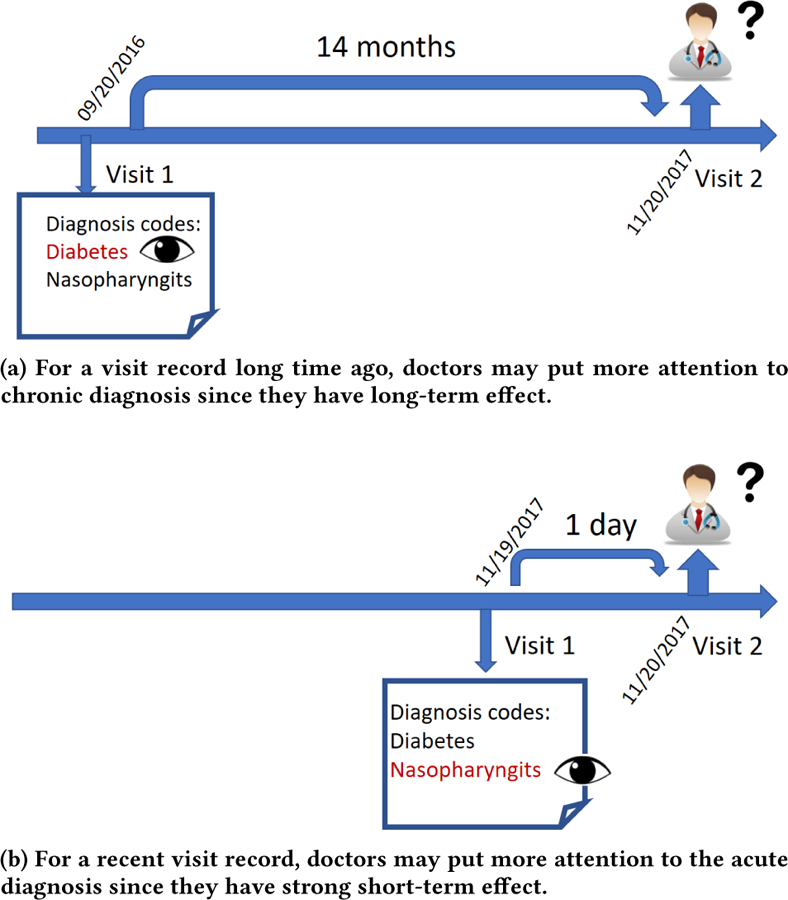
The diagnosis process in one visit: doctors review all previous patient visit records and pay attention to those diagnosis that may affect patient’s current health conditions. Here time interval plays an import role since each disease has its own effect range.
We evaluated Timeline on two data sets derived from SEER-Medicare medical claim data for 161,366 seniors diagnosed with breast cancer between 2000 and 2010. The specific task was to predict what is the primary diagnosis category for the hospital visit given all previous visits. Our results show that Timeline has higher accuracy than the state of the art deep learning models based on RNN. In addition, we demonstrate that time decay factors and attentions learned by Timeline are in accord with the medical knowledge and that Timeline can provide a useful insight into its predictions.
Our work makes the following contributions:
We propose Timeline, a novel interpretable end-to-end model to predict clinical events from past visits, while paying attention to elapsed time between visits and to types of conditions in the previous visits.
We empirically demonstrate that Timeline outperforms state of the art methods on two large real world medical claim datasets, while providing useful insights into its predictions.
The rest of the paper is organized as follows: in section 2 we discuss the relevant previous work. Section 3 presents the Timeline model. In section 4 we explain experiment design. The results are shown and discussed in section 5.
2. RELATED WORK
A unique feature of EHR is irregular sampling of patient visits. Several recent studies attempted to address this issue and proposed modifications to the traditional RNN model [2, 3, 8, 22, 35]. In [8] the authors propose an attention model combined with RNN to predict heart failure. The model learns attention at visit level and variable level. Therefore, the model could find influential past diagnoses and visits. Additionally, they propose a mechanism to handle time irregularity by using the time interval as an additional input feature. This simple approach improves the accuracy, but it does not improve interpretability. Other approaches modify the RNN hidden unit to incorporate time decay. For example, [3] applies a time decay factor to the previous hidden state in Gated Recurrent Unit (GRU) before calculating the new hidden state. [35] uses a time decay term in the update gate in GRU to find a tradeoff between the previous hidden state and the candidate hidden state. [22] modifies the forget gate of the standard LSTM unit to account for time irregularity of admissions. [2] first decomposes memory cell in LSTM into long-term memory and short-term memory, then applies time decay factor to discount the short term memory, and finally calculates the new memory by combining the long-term memory and a discounted short-term memory. In spite of the improved accuracy, the above approaches have limitations. [2, 22] use time decay factors insensitive to diseases, while the progression patterns of diseases should be different. [3, 35] focus on multivariate time series such as lab test results, while our paper focuses on medical codes. More importantly, [2, 3, 22, 35] apply time decay factors inside RNN units, which limits the interpretability of the resulting models, since RNN units are usually treated as black boxes. Instead of controlling how information flows inside the RNN units, our model controls how information of each disease flows into the model, therefore providing improved interpretation via analysis of weights associated with each code.
Recently, [24] developed an ensemble model for several healthcare prediction tasks. The ensemble model combines three different models, one of which is called Feedforward Model with Time-Aware Attention. Given the sequence of event embeddings, attention weights are calculated for each embedding while taking time into consideration. Our proposed model is different in three ways: 1) we use disease-dependent time decay factors, 2) we use LSTM instead of the feedforward neural network, 3) we use a sigmoid function to control how much information of each disease flows into the network, rather than the softmax function that transforms attention values into probabilities.
Several other models that use the attention mechanism to weight medical codes or visits have been proposed. [7] proposes Gram model which uses attention mechanism to utilize domain knowledge about the medical codes. For rare codes, the model could borrow information from the parent codes in the ontology. [19] proposes Dipole which employs bidirectional recurrent neural networks to remember all information from both the past and the future visits and introduces three attention mechanisms to calculate weights for each visit. [28] applies hierarchical attention networks [34] to learn both attention weights of medical codes and patient visits. All the above methods do not combine attention value with information about time intervals between visits.
Many other convolutional neural networks [4, 21] and recurrent neural networks [9, 25] have been applied to modeling EHR data for different prediction tasks, but their focus is slightly outside of the scope of this paper.
3. METHODOLOGY
In this section we describe the proposed Timeline model. We first introduce the problem setup and define our goal. Then, we describe the details of the proposed approach. Finally, we explain how to interpret the learned model by analyzing weights associated with medical codes.
3.1. Basic Problem Setup
Assume our dataset is a collection of patient records. The i-th patient consists of a sequence of Ti visits ordered by the visiting time. The j-th visit is a 2-tuple , in which consists of a set of unordered medical codes , which includes the diagnosis and procedure codes recorded during the visit and is the admission day of the visit. We denote the size of code vocabularly C as . For simplicity, in the following we describe our algorithm for a single patient and discard superscript i to avoid cluttering the notation.
3.2. Timeline Model
For a future visit Vi, the goal is to use the information in all previous visits V1, V2, V3,… Vi–1 to predict a future clinical event such as the primary diagnosis for visit Vi. Predicting the main diagnosis for a future visit as a function of the time of the future visit could be very useful in estimating the future risks of admission and coming up with preventive steps to avoid such visits. The state of the art solution to this task is to use a Recurrent Neural Network (RNN), which at each time step uses vector representation of a visit as input, combines the input with the RNN hidden state that encodes the past visits and transforms the RNN outputs into the prediction. One of the key steps in the RNN approach is to generate a vector representation for a given visit Vj. As shown in Figure 2, many previous studies use a simple approach that first embeds medical codes in a continuous vector space, wherein each unique code c in vocabulary C has a corresponding m-dimensional vector Then, for a given visit Vj, which contains N medical codes vector representation of the visit can be calculated by calculating the sum of embeddings of codes appearing in the visit as follows,
| (1) |
In the above approach, each code contributes equally to the final visit representation. However, some codes may be more important than other codes. For example, high blood pressure is much more indicative of hypertensive heart disease than insomnia. In our proposed model, called Timeline, each code contributes differently to the visit representation depending on when the medical code occurs and what the medical code is.
Figure 2:
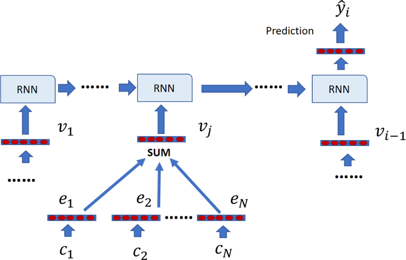
The framework of using vanilla visit representation with RNN for diagnosis prediction. Each visit representation is the sum of embeddings of medical codes in that visit.
The process of Timeline is shown in Figure 3. The first step is to aggregate context information for each code in the visit, because it has been observed that each disease may exhibit different meanings in different contexts. For example, sepsis can occur due to many different reasons such as infection from bacteria or viruses and can cause a wide range of symptoms from acute kidney injury to nervous system damage [11]. Previous methods use CNN filter [10] or RNN units [28] to generate the context vector. However, both CNN and RNN assume temporal or spatial order of input data while each visit is a set of unordered codes. Inspired by recent work [30], which uses attention mechanism to aggregate context information of words while not making an assumption that words are ordered, Timeline uses a similar way to calculate the context vector,
| (2) |
| (3) |
in which and . qn is the query vector for code cn and kn is the key vector for code cn. Next, attention value can be calculated as:
| (4) |
in which is the scaling factor.
Figure 3:
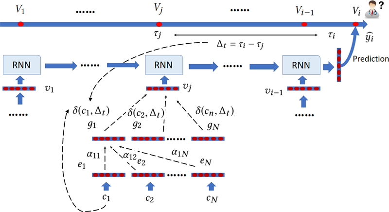
The illustration of Timeline. Timeline starts by embedding each medical code cn as a low dimensional vector en. Next, it uses a self attention mechanism to generate context vector gn. Then, it applies a disease progression function δ to control how much the information about cn flows into the RNN. δ depends on the specific disease c and the time interval ∆t. Finally, Timeline uses the weighted sum of the context vector as visit representation and feeds it into a RNN for prediction.
The context vector gn for code cn is calculated as the weighted sum of all codes in the same visit,
| (5) |
Next, we decide how much each code contributes to the final visit representation. We assume that each code has its own disease progression pattern, which can be modeled using δ function,
| (6) |
| (7) |
| (8) |
in which and are disease-specific learnable scalar parameters. ∆t is the time interval between visit Vj and the visit we need to do prediction for, is the initial influence of disease depicts how the influence of disease changes through time. If is small, then the effect of disease changes slowly through time. On the other hand, the effect of disease can dramatically change if is large. Finally, we use a sigmoid function S(x) to transform into a probability between 0 and 1. We did not use softmax function here since in softmax the sum of weights of codes in a visit is always 1. Instead, we want to reduce the information flow into the network if the visit happened long before the prediction time. represents how disease cn diagnosed at ∆t ago affects the patient condition at the time of prediction.
After calculating contributions of each code to the visit representation, can be calculated as
| (9) |
Finally, we use these visit representations as inputs to the RNN for prediction of the target label . Here yi is a one-hot vector in which only the target category is set to 1. In this paper we use bidirectional LSTM network [27] to provide prediction. Our goal is to predict primary diagnosis category yi out of L categories in visit Vi given all previous visits: . This process can be described as follows:
| (10) |
| (11) |
in which is the predicted category probability distribution, is the LSTM’s hidden state output at time step j, θLSTM are LSTM’s parameters, is the weight matrix, and is the bias vector of the output softmax function. Note that we use bidirectional LSTM network, although we can decide to use any RNN such as GRU [5]. Since our task is formulated as a multiclass classification problem, we use negative log likelihood loss function,
| (12) |
Note that equation (12) is the loss for one instance. In our implementation, we take the average of instance losses for multiple instances. In the next section we will describe how to generate instances from the raw data. We use the adaptive moment estimation (Adam) algorithm [14] to minimize the above loss values over all instances.
3.3. Interpretation
Interpretability is one of main requirements for healthcare predictive models. Interpretable model needs to shed some light on the rationale behind the prediction. In Timeline, this could be achieved by analyzing weights associated with each embedding e of medical code c. By combining equations (5) and (9), we get:
| (13) |
We define coefficient , which measures how much each code embedding ex contributes to the final visit representation: . If is large, the information of cx flows into the network substantially and contributes to the final prediction. We show some representative examples in section 4.4.
4. EXPERIMENTAL SETUP
4.1. Data Sets
In our experiments we used medical claims data from SEER-Medicare Linked Database [10]. SEER-Medicare Database records each visit of a patient as a set of diagnosis and procedure billing codes. In particular, our dataset contains inpatient, outpatient and carrier claims from 161,366 patients diagnosed with breast cancer from 2000 to 2010. The inpatient medical claims summarize services requiring a patient to be admitted to a hospital. Each inpatient claim summarizes one hospital stay and includes up to 25 ICD-9 diagnosis codes and 25 ICD-9 procedure codes. Outpatient claims summarize services which do not require a hospital stay. Outpatient claims contain a set of ICD-9 diagnosis, ICD-9 procedure, and CPT codes. CPT codes record medical procedures and are an alternative to the ICD-9 procedure ontology. Carrier claims refer to services by non-institutional providers such as physicians or registered nurses. Carrier claims use ICD-9 diagnosis codes and CPT codes. Given the heterogeneous nature of this database, we derived two datasets for our experiments.
Inpatient dataset: this dataset contains only inpatient visits. It evaluates the algorithm in the scenario where data come from a single source with homogeneous structure. This dataset contains only ICD-9 diagnosis codes and ICD-9 procedure codes.
Mixed dataset: this dataset is derived from all available visit types, including inpatient, outpatient and physician visits. This dataset allows us to evaluate the algorithm in a scenario where data come from different sources with heterogeneous structure. This dataset contains a mix of ICD-9 and CPT codes. To merge three different kinds of data, we combine all claims from a single day into a single visit. This is validated by an observation that inpatient or outpatient visits are often recorded as a mix or hospital and carrier claims.
Sequential diagnosis prediction task: our goal is to predict the primary diagnosis of future inpatient visits. Primary diagnosis is the main reason a patient got admitted into the hospital and is unique for each admission. Since a patient is typically admitted to a hospital only when he/she has a serious health condition, it is essential to understand the factors that lead to the hospitalization. As the vocabulary of ICD-9 diagnosis codes is very large, in this work we were content to predict the high level ICD-9 diagnosis categories, by grouping all ICD-9 diagnosis codes into 18 major disease groups1. For the Inpatient dataset, given a sequence of inpatient visits, we use all previous inpatient visits to predict the final recorded visit. For the Mixed dataset, we create an instance for each inpatient visit. In this way, one patient will result in two instances if he/she has two inpatient visits. For both datasets we exclude patients with less than two visits. The basic statistics of our datasets are shown in Table 1.
Table 1:
Basic statistics of Inpatient and Mixed datasets
| Dataset | Inpatient dataset | Mixed dataset |
|---|---|---|
| # of patients | 45,104 | 93,123 |
| # of visits | 155,898 | 5,979,529 |
| average # of visits per patient | 3.46 | 64.21 |
| max # of visits per visit | 35 | 483 |
| # of instances | 45,104 | 200,892 |
| # of unique medical codes | 6,020 | 18,826 |
| # of unique ICD-9 diagnosis codes | 3,928 | 8,342 |
| # of unique ICD-9 procedure codes | 2,092 | 2,614 |
| # of unique CPT codes | NA | 7,870 |
| Average # of medical codes per visit | 8.01 | 6.21 |
| Max # of medical codes per visit | 29 | 105 |
4.2. Experimental design
We start this subsection by describing the baselines for diagnosis prediction tasks. Then, we summarize the implementation details. We used the following five baselines:
Majority predictor: As a trivial baseline, we report the accuracy of a predictor that always predicts the majority class. Since our data relate to patients diagnosed with breast cancer, the majority class is “neoplasms”.
RNN-uni: This is the traditional RNN, which uses the sum of code embeddings as visit embeddings and feeds them as inputs to a unidirectional LSTM.
RNN-bi: This is the same as the RNN-uni method, except that we use a bidirectional LSTM to better represent information from the the first to the last visit.
Dipole [19]: Dipole employs three different attention mechanisms to calculate attention weights for each visit. Dipole also uses bidirectional RNN architecture to better represent information from all visits. We used location-based attention as baseline as it shows the best performance in [19].
GRNN-HA [28]: This model employs a hierarchal attention mechanism. It calculates two levels of attention: attention weights for medical codes and attention weights for patient visits.
We compared the five described baselines with our proposed Timeline model. Since the Timeline model uses a bidirectional architecture as the default, we also show the result of a Timeline model called Timeline-uni, which only uses a unidirectional LSTM.
To evaluate the accuracy of predicting the main diagnosis for the next visit, we used two measures for multiclass classification tasks: (1) accuracy, which equals the fraction of correct predictions, (2) weighted F1-score, which calculates F1-score for each class and reports their weighted mean.
We implemented all the approaches with Pytorch. We used Adam optimizer with the batch size of 48 patients. We randomly divided the dataset into the training, validation and test set in a 0.8, 0.1, 0.1 ratio. θ and µ were initialized as 1 and 0.1, respectively. We set the dimensionality of code embeddings m as 100, the dimensionality of attention query vectors and key vectors a as 100, and the dimensionality of hidden state of LSTM as 100. We used 100 iterations for each method and report the best performance.
4.3. Prediction results
We show the experimental results of 6 different approaches on Inpatient and Mixed datasets in Table 2.
Table 2:
The accuracy and weighted F1-score of Timeline and 5 baselines on two datasets.
| Inpatient dataset | Mixed dataset | |||
|---|---|---|---|---|
| Method | Accuracy | F1 | Accuracy | F1 |
| Majority Predictor | 0.212 | NA | 0.245 | NA |
| RNN-uni | 0.299 | 0.194 | 0.511 | 0.436 |
| RNN-bi | 0.298 | 0.199 | 0.516 | 0.442 |
| Dipole | 0.300 | 0.230 | 0.523 | 0.463 |
| GRNN-HA | 0.301 | 0.222 | 0.519 | 0.450 |
| Timeline-uni | 0.314 | 0.234 | 0.526 | 0.469 |
| Timeline | 0.315 | 0.235 | 0.530 | 0.473 |
From the table we can see that Timeline outperforms all baselines. The accuracies obtained on the Mixed dataset are much higher than on the Inpatient dataset, which demonstrates that using all available claims from multiple sources is very informative. We also observe that for Inpatient dataset, the benefit of using bidirectional model is not large. This could be explained by the fact that the number of claims per patient is much smaller in the Inpatient data than in the aims to improve representation of long sequences is marginal. On the other hand, for the Mixed dataset, bidirectional architectures outperform their unidirectional counterparts more significantly, which shows their superiority on long sequences of claims.
4.4. Model interpretation
In this subsection we discuss interpretability of Timeline. For each medical code we are able to calculate the weight associated with it using equation (13). We first generate two realistic-looking synthetic patients, which do not correspond to any real patient, but have properties similar to real patients in the SEER-Medicare dataset. We illustrate how our model utilizes the information in the patient visits for prediction. For each patient, we show each visit, the time stamp of each visit, medical codes recorded during each visit, and the weights assigned by Timeline to each medical code.
From Table 3 we can see that most of the medical codes have assigned weights equal to 0, meaning that they are ignored during the prediction. This weight sparsity is very useful for interpretation since our model focuses on medical codes with nonzero weights. Physicians could also gain insight by checking codes with nonzero weights. We can observe that our model has strong preference towards recent visits: visit 1 and visit 2 occurred 298 days ago and 185 days ago, respectively, and all weights of codes in these two visits are close to 0. For the visits 3–5, which occurred within the last month, Timeline gives large weights to medical codes indicative of female breast cancer. This result is enabled by the disease progression function δ in Timeline. Note that although visits 2 and 3 are consecutive visits, Timeline assigned large weights to codes in visit 3, while ignoring codes in visit 2, showing that it is aware that these two visits are distant in time.
Table 3:
Visits of synthetic patient 1. For each visit, all medical codes and weights associated with them are shown. CPT codes are prefixed by c_; ICD-9 diagnosis codes are prefixed by d_..
| visit 1 (298 days ago) | ||
| c_99213 | 0.0 | Office, outpatient visit |
| d_2859 | 0.0 | Anemia unspecified |
| c_92012 | 0.0 | Eye exam |
| visit 2 (185 days ago) | ||
| c_99213 | 0.0002 | Office, outpatient visit |
| d_4241 | 0.0002 | Aortic valve disorders |
| visit 3 (26 days ago) | ||
| c_80061 | 0.03 | Lipid panel |
| d_6117 | 1.739 | Signs and symptoms in breast disorders |
| visit 4 (10 days ago) | ||
| d_V048 | 0.458 | viral diseases |
| c_G0008 | 0.601 | Administration of influenza virus vaccine |
| d_4019 | 0.0 | Unspecified essential hypertension |
| visit 5 (8 days ago) | ||
| d_1742 | 1.87079 | Upper-inner quadrant of female breast cancer |
| c_99243 | 0.0 | Office consultation |
| Prediction: | Neoplasms (0.99) | |
From Table 4, we can observe that Timeline assigned weights to relatively few medical codes. Although visit 1 occurred 153 days ago, both medical codes d_7240 and d_4149 have large weights. The large weights were assigned because the two codes have slowly decaying disease progression function. For these two codes they can have large weights even when they are assigned long time ago since they have long-term influence on the future patient conditions. On the other hand, for the most recent visit, which occurred 18 days ago, none of the codes have large weights, since Timeline learned they have little influence on the future patient condition. This visit is about a basic blood test, which is not very influential for inferring the future health condition of the patient.
Table 4:
Visits of synthetic patient 2. For each visit, all medical codes and weights associated with them are shown. CPT codes are prefixed by c_; ICD-9 diagnosis codes are prefixed by d_.
| visit 1 (153 days ago) | ||
| d_4149 | 1.0 | Chronic ischemic heart disease unspecified |
| d_7240 | 1.0 | Spinal stenosis other than cervical |
| d_4019 | 0.0 | Unspecified essential hypertension |
| c_99213 | 0.0 | Office, outpatient visit |
| visit 2 (143 days ago) | ||
| d_2780 | 0.0 | Obesity |
| d_3751 | 0.0 | Disorders of lacrimal gland |
| c_92012 | 0.0 | Eye exam |
| visit 3 (82 days ago) | ||
| d_3771 | 1.94464 | Pathologic fracture |
| c_72080 | 1.739 | Radiologic examination, spine |
| d_4019 | 0.0 | Unspecified essential hypertension |
| visit 4 (18 days ago) | ||
| d_4019 | 0.0 | Unspecified essential hypertension |
| c_80048 | 0.017 | Basic metabolic panel |
| c_85025 | 0.0 | Blood count |
| d_V726 | 0.301 | Special investigations and examinations |
| Prediction: | diseases of the musculoskeletal system and connective tissue (0.67) | |
As another illustration of the interpretability of Timeline, we generated another synthetic patient. As seen in Table 5, the patient has 2 recorded visits, the first occurred t days ago with diagnosis d_1749 (female breast cancer, unspecified), while the second occurred 10 days ago with diagnosis d_2720 (Pure hypercholesterolemia). d_1749 is a strong indicator of cancer hospital admission while d_2720 is an indicator of admission because of circulatory system disease. The prediction task is to predict the main diagnosis of the next hospital visit if the first visit occurs t ago, where t ranges form 11 to 160. We can observe in Figure 4 that for t < 60 the Timeline is very confident the diagnosis will be “neoplasms”, while for t > 80 it is very confident it will be “diseases of the circulatory system”. This example shows that Timeline is very sensitive to the exact time of past clinical events.
Table 5:
We generate two visits, one visit contains d_1749 and one visit contains d_2720, we change the time interval of the first visit in order to see how prediction changed.
| visit 1 (t days ago) | |
| d_1749 | female breast cancer unspecified |
| visit 2 (10 days ago) | |
| d_2720 | Pure hypercholesterolemia |
Figure 4:
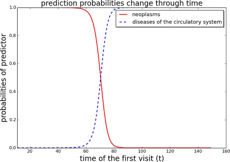
We change time interval t in Table 5 and show how prediction probabilities change with t.
To further illustrate how the learned disease progression functions might differ depending on the disease, we select six medical codes and show their δ (c, ∆) function in Figure 5. As we can see, each disease has its own disease progression function. For d_5712 (alcoholic cirrhosis of liver), δ decrease slowly through time and approaches zero after 100 days. However, for acute diseases d_4878 (influenza) and d_4643 (acute epiglottitis), it decreases much faster and approaches zero in 20 days and 10 days, respectively. For code d_4280 (congestive heart failure unspecified), its influence actually increases over time and reaches 1 (the upper limit of sigmoid function δ ) very fast. This implies d_4280 is a very serious chronic disease and its influence is high irrespective of time. We note that this result is a consequence of our decision to allow the µ parameter in equation (6) to be negative. For d_4019 (essential hypertension unspecified), we found its influence decreases fast and starts from a relatively low value. This is explained by the fact that hypertension is a very common comorbidity and that it is not predictive of the future hospitalizations. Therefore, Timeline decreases its influence fast and tries to ignore it. Another common code is our dataset is d_1749 (female breast cancer unspecified). δ of this code decreases slowly and approaches zero at 100 days. This code is a very strong indicator of neoplasm, and its influences stays strong over a long time period.
Figure 5:
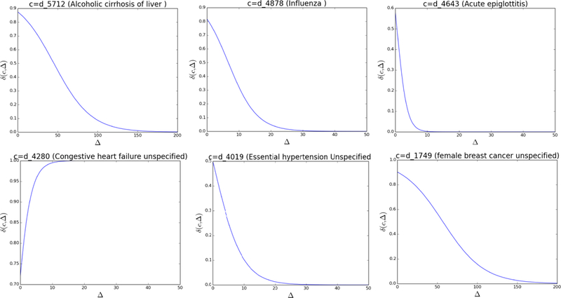
The δ (c, ∆) function for six different codes.
5. CONCLUSIONS
Predictive modeling, such as prediction of the main diagnosis of a future hospitalization, is one of the key challenges in healthcare informatics. In order to properly model sequential patient data, it is important to take sampling irregularity and different disease progression patterns into consideration. The state of the art deep learning approaches for predictive modeling of EHR data are not capable of producing interpretable models that can account for those factors. To address this issue, in this paper we proposed Timeline, a novel interpretable model which uses an attention mechanism to aggregate context information of medical codes and uses time-aware disease-specific progression function to model how much information of each disease flows into the recurrent neural network. Our experiments demonstrate that our model outperforms state-of-the-art deep neural networks on the task of predicting the main diagnosis of a future hospitalization using two large scale real world data sets. We also demonstrated the interpretability of Timeline by analyzing weights associated with different medical codes recorded in previous visits.
ACKNOWLEDGMENTS
This work was supported by the National Institutes of Health grants R21CA202130 and P30CA006927. We thank Dr. Richard Bleicher from Fox Chase Cancer Center for providing us with access to the patient data.
Footnotes
Contributor Information
Tian Bai, Temple University, Philadelphia, PA, USA tue98264@temple.edu.
Brian L. Egleston, Fox Chase Cancer Center Philadelphia, PA, USA Brian.Egleston@fccc.edu
Shanshan Zhang, Temple University, Philadelphia, PA, USA zhang.shanshan@temple.edu.
Slobodan Vucetic, Temple University, Philadelphia, PA, USA vucetic@temple.edu.
REFERENCES
- [1].Bahdanau Dzmitry, Cho Kyunghyun, and Bengio Yoshua. 2014. Neural machine translation by jointly learning to align and translate. arXiv preprint arXiv:1409.0473 (2014).
- [2].Baytas Inci M, Xiao Cao, Zhang Xi, Wang Fei, Jain Anil K, and Zhou Jiayu. 2017. Patient subtyping via time-aware LSTM networks In Proceedings of the 23rd ACM SIGKDD International Conference on Knowledge Discovery and Data Mining. ACM, 65–74. [Google Scholar]
- [3].Che Zhengping, Purushotham Sanjay, Cho Kyunghyun, Sontag David, and Liu Yan. 2016. Recurrent neural networks for multivariate time series with missing values. arXiv preprint arXiv:1606.01865 (2016). [DOI] [PMC free article] [PubMed]
- [4].Cheng Yu, Wang Fei, Zhang Ping, and Hu Jianying. 2016. Risk prediction with electronic health records: A deep learning approach In Proceedings of the 2016 SIAM International Conference on Data Mining. SIAM, 432–440. [Google Scholar]
- [5].Cho Kyunghyun, Merriënboer Bart Van, Gulcehre Caglar, Bahdanau Dzmitry, Bougares Fethi, Schwenk Holger, and Bengio Yoshua. 2014. Learning phrase representations using RNN encoder-decoder for statistical machine translation. arXiv preprint arXiv:1406.1078 (2014).
- [6].Choi Edward, Bahadori Mohammad Taha, Schuetz Andy, Stewart Walter F, and Sun Jimeng. 2016. Doctor ai: Predicting clinical events via recurrent neural networks In Machine Learning for Healthcare Conference. 301–318. [PMC free article] [PubMed] [Google Scholar]
- [7].Choi Edward, Bahadori Mohammad Taha, Song Le, Stewart Walter F, and Sun Jimeng. 2017. GRAM: Graph-based attention model for healthcare representation learning In Proceedings of the 23rd ACM SIGKDD International Conference on Knowledge Discovery and Data Mining. ACM, 787–795. [DOI] [PMC free article] [PubMed] [Google Scholar]
- [8].Choi Edward, Bahadori Mohammad Taha, Sun Jimeng, Kulas Joshua, Schuetz Andy, and Stewart Walter. 2016. Retain: An interpretable predictive model for healthcare using reverse time attention mechanism. In Advances in Neural Information Processing Systems 3504–3512.
- [9].Choi Edward, Schuetz Andy, Stewart Walter F, and Sun Jimeng. 2016. Using recurrent neural network models for early detection of heart failure onset. Journal of the American Medical Informatics Association 24, 2 (2016), 361–370. [DOI] [PMC free article] [PubMed] [Google Scholar]
- [10].Feng Yujuan, Min Xu, Chen Ning, Chen Hu, Xie Xiaolei, Wang Haibo, and Chen Ting. 2017. Patient outcome prediction via convolutional neural networks based on multi-granularity medical concept embedding. In 2017 IEEE International Conference on Bioinformatics and Biomedicine (BIBM). IEEE, 770–777. [Google Scholar]
- [11].Gligorijevic Djordje, Stojanovic Jelena, and Obradovic Zoran. 2016. Disease types discovery from a large database of inpatient records: A sepsis study. Methods 111 (2016), 45–55. [DOI] [PubMed] [Google Scholar]
- [12].Halpern Yoni, Horng Steven, Choi Youngduck, and Sontag David. 2016. Electronic medical record phenotyping using the anchor and learn framework. Journal of the American Medical Informatics Association 23, 4 (2016), 731–740. [DOI] [PMC free article] [PubMed] [Google Scholar]
- [13].Hochreiter Sepp and Schmidhuber Jürgen. 1997. Long short-term memory. Neural computation 9, 8 (1997), 1735–1780. [DOI] [PubMed] [Google Scholar]
- [14].Kingma Diederik P and Ba Jimmy. 2014. Adam: A method for stochastic optimization. arXiv preprint arXiv:1412.6980 (2014).
- [15].Klabunde Carrie N, Potosky Arnold L, Legler Julie M, and Warren Joan L. 2000. Development of a comorbidity index using physician claims data. Journal of clinical epidemiology 53, 12 (2000), 1258–1267. [DOI] [PubMed] [Google Scholar]
- [16].Krumholz Harlan M, Wang Yun, Mattera Jennifer A, Wang Yongfei, Han Lein Fang, Ingber Melvin J, Roman Sheila, and Normand Sharon-Lise T. 2006. An administrative claims model suitable for profiling hospital performance based on 30-day mortality rates among patients with heart failure. Circulation 113, 13 (2006), 1693–1701. [DOI] [PubMed] [Google Scholar]
- [17].Levitan Nathan, Dowlati A, Remick SC, Tahsildar HI, Sivinski LD, Beyth R, and Rimm AA. 1999. Rates of initial and recurrent thromboembolic disease among patients with malignancy versus those without malignancy. Risk analysis using Medicare claims data. Medicine (Baltimore) 78, 5 (1999), 285–91. [DOI] [PubMed] [Google Scholar]
- [18].Lipton Zachary C, Kale David C, Elkan Charles, and Wetzel Randall. 2015. Learning to diagnose with LSTM recurrent neural networks. arXiv preprint arXiv:1511.03677 (2015).
- [19].Ma Fenglong, Chitta Radha, Zhou Jing, You Quanzeng, Sun Tong, and Gao Jing. 2017. Dipole: Diagnosis prediction in healthcare via attention-based bidirectional recurrent neural networks. In Proceedings of the 23rd ACM SIGKDD International Conference on Knowledge Discovery and Data Mining. ACM, 1903–1911. [Google Scholar]
- [20].Miotto Riccardo, Wang Fei, Wang Shuang, Jiang Xiaoqian, and Dudley Joel T. 2017. Deep learning for healthcare: review, opportunities and challenges. Briefings in bioinformatics (2017). [DOI] [PMC free article] [PubMed]
- [21].Nguyen Phuoc, Tran Truyen, Wickramasinghe Nilmini, and Venkatesh Svetha. 2017. Deepr: A Convolutional Net for Medical Records. IEEE journal of biomedical and health informatics 21, 1 (2017), 22–30. [DOI] [PubMed] [Google Scholar]
- [22].Pham Trang, Tran Truyen, Phung Dinh, and Venkatesh Svetha. 2016. Deepcare: A deep dynamic memory model for predictive medicine. In Pacific-Asia Conference on Knowledge Discovery and Data Mining. Springer, 30–41. [Google Scholar]
- [23].Purushotham Sanjay, Meng Chuizheng, Che Zhengping, and Liu Yan. 2017. Bench-mark of Deep Learning Models on Large Healthcare MIMIC Datasets. arXiv preprint arXiv:1710.08531 (2017). [DOI] [PubMed]
- [24].Rajkomar Alvin, Oren Eyal, Chen Kai, Dai Andrew M, Hajaj Nissan, Liu Peter J, Liu Xiaobing, Sun Mimi, Sundberg Patrik, Yee Hector, et al. 2018. Scalable and accurate deep learning for electronic health records. arXiv preprint arXiv:1801.07860 (2018). [DOI] [PMC free article] [PubMed]
- [25].Razavian Narges, Marcus Jake, and Sontag David. 2016. Multi-task prediction of disease onsets from longitudinal laboratory tests. In Machine Learning for Healthcare Conference. 73–100. [Google Scholar]
- [26].Schneeweiss Sebastian, Seeger John D, Maclure Malcolm, Wang Philip S, Avorn Jerry, and Glynn Robert J. 2001. Performance of comorbidity scores to control for confounding in epidemiologic studies using claims data. American journal of epidemiology 154, 9 (2001), 854–864. [DOI] [PubMed] [Google Scholar]
- [27].Schuster Mike and Paliwal Kuldip K. 1997. Bidirectional recurrent neural networks. IEEE Transactions on Signal Processing 45, 11 (1997), 2673–2681. [Google Scholar]
- [28].Sha Ying and Wang May D. 2017. Interpretable Predictions of Clinical Outcomes with An Attention-based Recurrent Neural Network. In Proceedings of the 8th ACM International Conference on Bioinformatics, Computational Biology, and Health Informatics. ACM, 233–240. [DOI] [PMC free article] [PubMed] [Google Scholar]
- [29].Taylor Donald H Jr, Østbye Truls, Langa Kenneth M, Weir David, and Plassman Brenda L. 2009. The accuracy of Medicare claims as an epidemiological tool: the case of dementia revisited. Journal of Alzheimer’s Disease 17, 4 (2009), 807–815. [DOI] [PMC free article] [PubMed] [Google Scholar]
- [30].Vaswani Ashish, Shazeer Noam, Parmar Niki, Uszkoreit Jakob, Jones Llion, Gomez Aidan N, Kaiser Łukasz, and Polosukhin Illia. 2017. Attention is all you need. In Advances in Neural Information Processing Systems 6000–6010.
- [31].Warren Joan L, Harlan Linda C, Fahey Angela, Virnig Beth A, Freeman Jean L, Klabunde Carrie N, Cooper Gregory S, and Knopf Kevin B. 2002. Utility of the SEER-Medicare data to identify chemotherapy use. Medical care 40, 8 (2002), IV–55. [DOI] [PubMed] [Google Scholar]
- [32].Yadav Pranjul, Steinbach Michael, Kumar Vipin, and Simon Gyorgy. 2017. Mining Electronic Health Records: A Survey. arXiv preprint arXiv:1702.03222 (2017).
- [33].Yan Yan, Birman-Deych Elena, Radford Martha J, Nilasena David S, and Gage Brian F. 2005. Comorbidity indices to predict mortality from Medicare data: results from the national registry of atrial fibrillation. Medical care 43, 11 (2005), 1073–1077. [DOI] [PubMed] [Google Scholar]
- [34].Yang Zichao, Yang Diyi, Dyer Chris, He Xiaodong, Smola Alex, and Hovy Eduard. 2016. Hierarchical attention networks for document classification. In Proceedings of the 2016 Conference of the North American Chapter of the Association for Computational Linguistics: Human Language Technologies. 1480–1489. [Google Scholar]
- [35].Zheng Kaiping, Wang Wei, Gao Jinyang, Ngiam Kee Yuan, Ooi Beng Chin, and James Yip Wei Luen. 2017. Capturing Feature-Level Irregularity in Disease Progression Modeling. In Proceedings of the 2017 ACM on Conference on Information and Knowledge Management. ACM, 1579–1588. [Google Scholar]