Isotropic periodic sum: A method for the calculation of long-range interactions

Abstract

This work presents an accurate and efficient approach to the calculation of long-range interactions for molecular modeling and simulation. This method defines a local region for each particle and describes the remaining region as images of the local region statistically distributed in an isotropic and periodic way, which we call isotropic periodic images. Different from lattice sum methods that sum over discrete lattice images generated by periodic boundary conditions, this method sums over the isotropic periodic images to calculate long-range interactions, and is referred to as the isotropic periodic sum (IPS) method. The IPS method is not a lattice sum method and eliminates the need for a reciprocal space sum. Several analytic solutions of IPS for commonly used potentials are presented. It is demonstrated that the IPS method produces results very similar to that of Ewald summation, but with three major advantages, (1) it eliminates unwanted symmetry artifacts raised from periodic boundary conditions, (2) it can be applied to potentials of any functional form and to fully and partially homogenous systems as well as finite systems, and (3) it is more computationally efficient and can be easily parallelized for multiprocessor computers. Therefore, this method provides a general approach to an efficient calculation of long-range interactions for various kinds of molecular systems.

I. INTRODUCTION

Molecular simulation has been widely used in the study of many-particle systems.^1,2 Long-range interactions, such as electrostatic and van der Waals (VDW) interactions, are usually the most costly part of a molecular simulation. Electrostatic interaction is especially troublesome since its range reaches far beyond the size of a typical simulation system. There are many approaches for long-range interaction calculation,¹ such as cutoff methods,^3–6 reaction field methods,^7–11 and lattice sum methods.^1,2,12,13 The cutoff methods calculate interactions within a cutoff range and approximate the interactions beyond the cutoff range as zero or, after long-range correction, a constant. The reaction field methods assume a continuum dielectric medium with a predefined dielectric constant beyond the cutoff range and long-range interactions are replaced by reaction field interactions. The lattice sum methods use discrete lattice images created by periodic boundary conditions (PBC) to calculate long-range interactions. Among these methods, the lattice sum methods are widely recognized to be the most accurate.

Lattice sum methods calculate long-range interactions by summing over all interactions with the lattice images generated by periodic boundary conditions. Obviously, lattice sum methods do not apply to systems with irregular boundaries or no boundaries such as vacuum. For periodic boundary systems, an accurate summation over all lattice images is difficult to compute. To improve calculation efficiency, many methods such as particle-mesh Ewald,^14,15 particle-particle-particle-mesh Ewald,¹⁶ and fast multipole method¹⁷ have been developed for the electrostatic potential. While for other potential forms such as the Lennard-Jones potential, the calculation is complicated by the diversity of atom sizes. In addition, the lattice sum methods exaggerate the symmetry effect imposed by periodic boundary conditions. When noncrystalline systems such as liquids and solutions are simulated under periodic boundary conditions, they may give rise to unwanted long-range correlation artifacts¹⁸ as well as anisotropy effects due to the artificially induced periodicity.¹⁹ This anisotropy effect is especially troublesome when studying macromolecular systems where conformational distributions are very sensitive to image interactions.

In this work, we present an approach called isotropic periodic sum (IPS) to calculate long-range interactions. Unlike lattice sum methods, this method does not sum the lattice images. Instead, this method uses so-called isotropic periodic images to represent remote structures statistically in calculating long-range interactions. The isotropic and periodic characters of the images make the summation of long-range interactions a much easier problem than the summation over the discrete lattice images. This method simplifies particle interactions to short-range interactions within a defined region plus long-range interactions given by the isotropic periodic sums.

In the following sections, we first describe the IPS method and calculation details. Then, through several examples, we examine the accuracy of IPS in energy and force calculation for homogeneous as well as heterogeneous systems. Finally, we evaluate the application of the IPS method through simulations of two example systems.

II. THEORIES AND METHODS

A. Isotropic periodic images and isotropic periodic sum

In a molecular system, the energy of a particle is the sum of interactions with all other particles. For a particle i, it is convenient to define a local region Ω_i centered at this particle, so that the interactions with particle i can be divided into local interactions within the local region and long-range interactions outside the local region:

$$E_i=\frac{1}{2}\sum _j^{\infty }{\epsilon }_{ij}({\mathbf{r}}_{ij})=\frac{1}{2}\sum _{{\mathbf{r}}_j\in {\mathbf{\Omega }}_i}{\epsilon }_{ij}({\mathbf{r}}_{ij})+\frac{1}{2}\sum _{{\mathbf{r}}_j\notin {\mathbf{\Omega }}_i}{\epsilon }_{ij}({\mathbf{r}}_{ij}),$$ (1)

where r_j is the position of particle j and r_ij is the vector from particle i to particle j. Normally, all short-range interactions such as covalent bonding interactions, as well as all other interactions with the local particles, are included in the local region interactions shown as the first term in the right-hand side of Eq. (1). The second term includes only long-range interactions, such as electrostatic and VDW potentials, with all particles outside the local region. Theoretically, the long-range contribution, the second term in the right-hand side of Eq. (1), should cover the whole system, which is unrealistic to calculate explicitly for normal systems of interest.

The summation over a large number of interactions beyond the local region can be simplified by assuming that the particle configurations outside the local region are somehow related to the configurations in the local region, so that the long-range contribution becomes a function of the configuration of the local region:

$$\begin{gathered} E_i=\frac{1}{2}\sum _{{\mathbf{r}}_j\in {\mathbf{\Omega }}_i}{\epsilon }_{ij}({\mathbf{r}}_{ij})+\frac{1}{2}\sum _{{\mathbf{r}}_j\in {\mathbf{\Omega }}_i}{\varphi }_{ij}({\mathbf{r}}_{ij},{\mathbf{\Omega }}_i) \\ =\frac{1}{2}\sum _{{\mathbf{r}}_j\in {\mathbf{\Omega }}_i}[{\epsilon }_{ij}({\mathbf{r}}_{ij})+{\varphi }_{ij}({\mathbf{r}}_{ij},{\mathbf{\Omega }}_i)]. \end{gathered}$$ (2)

Here, ϕ_ij(r_ij, Ω_i) represents the long-range contribution as a function of r_ij and Ω_i. The cutoff methods use a spherical local region of radius r_c, and assume ϕ_ij(r_ij, Ω_i) = 0 or ${\varphi }_{ij}({\mathbf{r}}_{ij},{\mathbf{\Omega }}_i)={\epsilon }_{ij}^{\text{LRC}}(r_c)$ where ${\epsilon }_{ij}^{\text{LRC}}(r_c)$ is the long-range correction (LRC) term based on a uniform distribution¹ or calculated using a longer cutoff distance.²⁰ The reaction field methods assume a continuum dielectric medium surrounding the local region and ϕ_ij(r_ij, Ω_i) represents the interaction with the medium. The lattice sum methods assume a local region defined by a periodic boundary condition and ϕ_ij(r_ij, Ω_i) represents the sum over interactions with all lattice images created by the periodic boundary condition. Obviously, these methods are different in the way a local region is defined and the estimation of the long-range contributions.

For an isotropic, homogeneous system consisting of many particles, there is no structural preference in any direction. Statistically, two regions far away may be similar in structure. To calculate the interactions of a particle, assuming any region far away from it be an image of its local region is a reasonable approximation. The widely used periodic boundary condition is a special case of this approximation, which assumes that the images of the local regions are arranged to follow a given lattice symmetry. Instead of using the static lattice images created by periodic boundary conditions, we use so-called isotropic periodic images of a local region as described below to calculate long-range interactions.

In a homogenous system, for each particle, the near region around it is defined as its local region and the remaining region is represented by a distribution of images of this local region. The size of the local region determines how much heterogeneity will be considered. Because the system is isotropic, the local region should be spherical and the images of the local region, which we call image regions, should distribute statistically around the local region in all directions. If we denote the radius of the local region as r_c, based on periodicity, the nearest image regions are bound with the local region and their centers must be 2r_c from the center of the local region. Because the image regions distribute in all directions, the centers of the nearest image regions will form an image shell with a radius of 2r_c. Similarly, the next image shell has a radius of 4r_c and the mth shell has a radius of 2mr_c. Because all image regions are the same as the local region and have a radius of r_c, the space with a radius from (2m−1)r_c to (2m+1)r_c belongs to the mth image shell. The image regions on image shells are simply translations of the local region without any rotation. Therefore, the images of each particle in the local region form its own image shells centered at this particle. Because of the isotropic and periodic distribution, we call these images the isotropic periodic images. It should be noted that these isotropic periodic images are only used to represent statistically the conformation beyond the local region for long-range interaction calculation. They are not actually present in a simulation system.

Figure 1 illustrates the definition of the local region and its isotropic periodic images in a square periodic boundary system. The local region of particle 1 is enclosed by a dashed circle of radius r_c. The isotropic periodic images of the local region and its particles are shown as dotted circles and dotted particles labeled correspondingly. The image regions of the first layer are bounded with the local region and occupy the area with a radius from r_c to 3r_c. In this layer, the isotropic periodic images of particle 1 are distributed on image shells with a radius of 2r_c. The image regions on an image shell are statistical representation of conformations around this image shell and can overlap with each other. Because the image regions are translation of the local region, the images of each particle will distribute on its own image shells centered at this particle. As shown in Fig. 1, the isotropic periodic images of particle 2 distribute on image shells centered at particle 2. Particle 1 only interacts with particles within its local region, i.e., particles 2, 3, and 4, and the isotropic periodic images of all particles in its local region, including itself. Similarly, all particles in the local region will interact with the isotropic periodic images of particle 1. All other particles, such as particles 5, 6, 7, and all images generated by the periodic boundary condition that are outside the local region are not seen by particle 1 and are replaced by the isotropic periodic images of the local particles in the calculation of long-range energies. Particle 4 is at the boundary of the local region of particle 1 and has the same distance r_c from particle 1 and from its nearest isotropic periodic image on the first image shell. Due to the periodicity, the total force on particle 4 from particle 1 and its images is zero. Please note that the total interaction between particle 1 and all images of particle 2 will be the same as that between particle 2 and all images of particle 1.

FIG. 1.

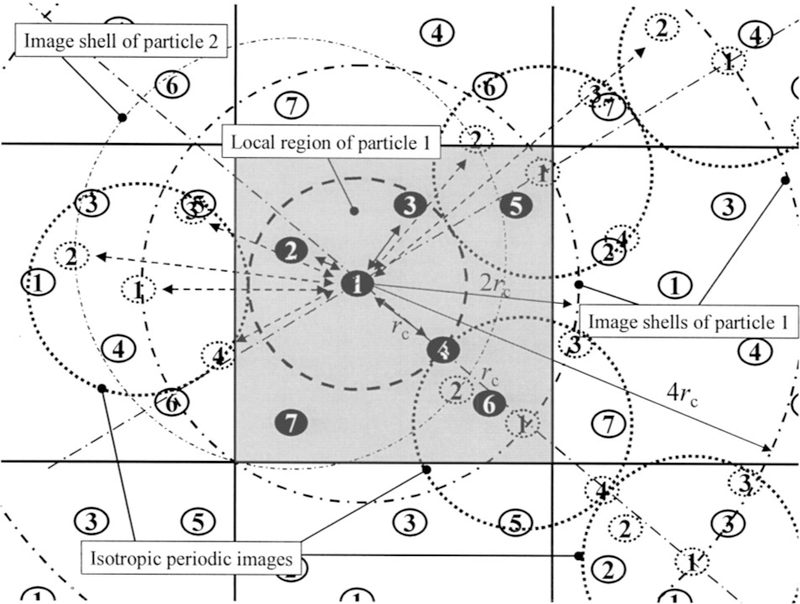
The local region and isotropic periodic images in a square periodic boundary system. The local region of particle 1 is enclosed by the dashed circle. The image shells of particles 1 and 2 are shown as dotted-dashed circles around particles 1 and 2, respectively. The image shells of other particles are not shown for clarity. The isotropic periodic images of the local region shown as dotted circles distribute around the local region and can overlap with each other. Particle 1 interacts with particles 2, 3, and 4 in its local region and the isotropic periodic image particles, shown as dotted particles. Particle 4 is at the boundary of the local region and has the same distances to particle 1 and to the nearest image of particle 1.

Some systems are homogenous only in certain directions, which we call partially homogenous systems. For example, planar membranes are often homogenous along their planar directions, and a metal wire can be thought to be homogenous along the elongate direction. To be general, we define a homogenous index (p_x, p_y, p_z) to describe a partially homogenous system. The index component is 1 if it is homogenous along this component direction or 0 otherwise. For example, a fully homogenous system which we call a three-dimensional (3D) homogenous system has a homogenous index of (1,1,1); for a membrane on the x–y plane, which we call a 2D homogenous system, the homogenous index is (1,1,0); and for a metal wire along the z axis, which we call a 1D homogenous system, the homogenous index is (0,0,1). Note that all systems we discuss here are in three-dimensional space, while the number of homogenous dimensions is 1, 2, or 3 for 1D, 2D, or 3D homogenous systems, respectively.

Based on the homogenous index, we separate a Cartesian coordinate r=(x, y, z) to an isotropic coordinate u (p_xx, p_yy, p_zz) and an anisotropic coordinate h=[(1–p_x)x,(1–p_y) y,(1–p_z)z]. Correspondingly, we have the isotropic distance

$$u_{ij}=\sqrt{p_x^2{(x_j-x_i)}^2+p_y^2{(y_j-y_i)}^2+p_z^2{(z_j-z_i)}^2}$$ (3)

and the anisotropic distance

$$h_{ij}=\sqrt{{(1-p_x)}^2{(x_j-x_i)}^2+{(1-p_y)}^2{(y_j-y_i)}^2+{(1-p_z)}^2{(z_j-z_i)}^2},$$ (4)

where (x_i, y_i, z_i) and (x_j, y_j, z_j) are the coordinates of particles i and j, respectively. Because the homogenous indices p_x, p_y, and p_z are either 0 or 1, we have the following relation:

$$r_{ij}=\sqrt{{(x_j-x_i)}^2+{(y_j-y_i)}^2+{(z_j-z_i)}^2}=\sqrt{u_{ij}^2+h_{ij}^2}.$$ (5)

Any potential function of distance r is also a function of u and h: ε(r)= ε(u,h).

In partially homogenous systems, the local region of any particle i includes all particles j whose isotropic distance u_ij is less than the cutoff distance r_c. For a 3D homogenous system, the local region is a sphere with a radius r_c. For a 2D homogenous system, the local region is a cylinder of radius r_c with an infinite length perpendicular to the homogeneous plane. And for a 1D homogenous system, the local region is a cylinder of length 2r_c along the homogeneous axis with an infinite radius. Here, the partially homogenous systems are those with small system sizes in the anisotropic direction, as the 1D or 2D CaCl₂ fluids shown later in this paper. Even though the local regions are infinitely large in these directions, the particles contained in the local region are limited. When the system size in the anisotropic direction is large, for example, periodic, the system would be better treated approximately as a fully (3D) homogenous system to avoid a large number of particles in a local region.

Figure 2 shows a partially homogenous system of two particles. Two particles A and B are separated by an isotropic distance u and an anisotropic distance h. Between A and all images of B, the anisotropic distances are same, while the isotropic distances are different. If u is less than the cutoff distance r_c, particle B will be in the local region of particle A. The total interaction between A and B is the sum of the direct interaction between them and all interactions with their images:

$${\epsilon }^{\text{IPS}}(\mathbf{r})=\epsilon (r)+\sum _m\epsilon (u_m,h)=\epsilon (r)+\varphi (u,h).$$ (6)

Here, u_m is the isotropic distance between particle A and the mth image of particle B. The summation ϕ(u,h) = Σ_mε(u_m,h) runs over all isotropic periodic images of particle B and is called an isotropic periodic sum.

FIG. 2.

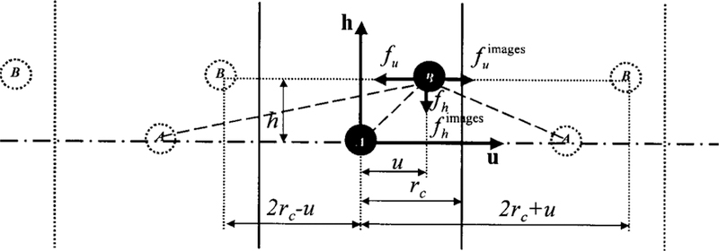
A partially homogenous system of two particles, A and B, viewed on the u×h plan. The system is periodic in the u direction and vertical lines mark the boundaries. The images labeled ‘‘B’’ are images of particle B, and images labeled ‘‘A’’ are images of particle A. B interacts with A and all images. In u direction (horizontal), the forces from A and from A’s images have opposite direction and when B is at the boundary (u=r_c) they cancel with each other. In h direction (vertical), the forces from A and from A’s images have same direction and will not cancel when B is at the boundary.

For any particle in a local region of volume V₀, its density is 1/V₀. On each image shell, the number of images can be calculated from the volume of the image shell:

$$n(m)=\frac{V_m}{V_0},$$ (7)

where V_m is the volume of the mth image shell defined as the region where the isotropic distance runs from (2m−1)r_c to (2m+1)r_c. For different type of homogenous systems, we can calculate the shell image numbers according to equations listed below:

$$n_{1\text{D}}(m)=\frac{2\left[\left(2m+1\right)r_c-(2m-1)r_c\right]}{2r_c}=2,$$ (8)

$$n_{2\text{D}}(m)=\frac{\pi {\left(2m+1\right)}^2{r}_c^2-\pi {(2m-1)}^2{r}_c^2}{\pi r_c^2}=8m,$$ (9)

$$n_{3\text{D}}(m)=\frac{\frac{4}{3}\pi {\left(2m+1\right)}^2{r}_c^3-\frac{4}{3}\pi {(2m-1)}^3{r}_c^2}{\frac{4}{3}\pi r_c^3}=24m^2+2.$$ (10)

The distribution of the n(m) images on image shells effects the particle-image interaction. Because there are more than one images on each image shell, the image distribution cannot be fully random due to the mutual exclusion between images. We divide the distribution of the images on each image shell into two parts, a random distribution and a non-random distribution. For a pair of interacting particles, the image distribution should be symmetric about the axis connecting the two particles. The simplest nonrandom distribution that is symmetric about the axis would be the one with particles distributing on the axis, i.e., with particles sitting at the two points where the axis crosses the shell, as shown in Fig. 3. We call this kind of distribution the axial distribution. For simplicity, we use the axial distribution to describe approximately the effect due to the nonrandom distribution of the images. On each image shell, assume there are ξ images on each of the two axis-crossing positions. We call ξ the distribution parameter, which describes the nonrandomness of the image distribution. The rest images n(m)−2 ξ distribute randomly on the shell.

FIG. 3.

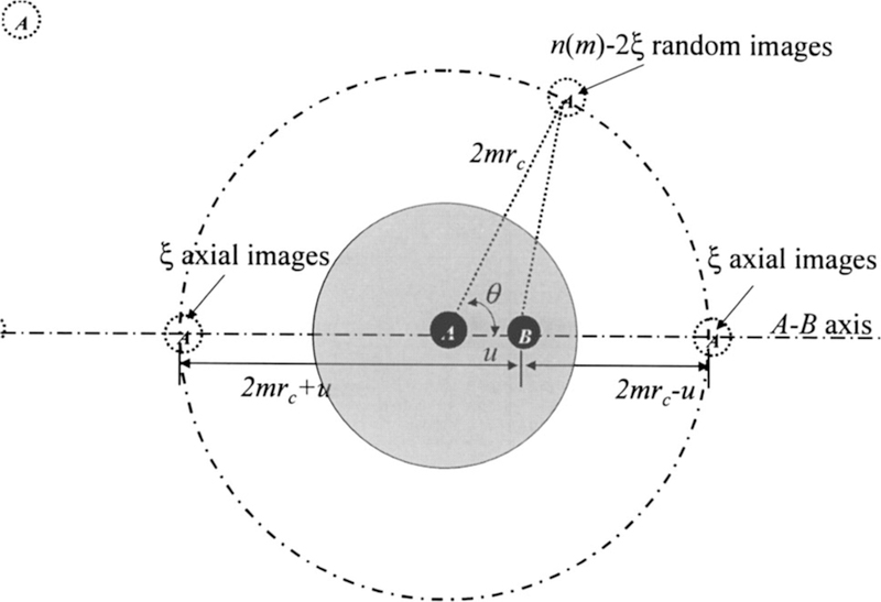
The distribution of isotropic periodic images of particle A on its image shells. The distribution is a combination of a random distribution and a nonrandom distribution. The nonrandom distribution is represented by 2ξ particle images sitting at the two points where the axis connecting particles A and B crossing the shell. The rest n(m)−2ξ images distribute randomly on the shell. Particle B interacts with all images of particle A. The image shells of particle B are not shown here, which would be centered at particle B. Please note that the interaction energy between particle B and all images of particle A is the same as that between particle A and all images of particle B.

The isotropic distances between particle A and the two axial images of particle B on the mth shell are 2mr_c−u and 2mr_c+u (see Fig. 3). The sum of the interactions between A and all axial images of B is called the axial interaction:

$$\begin{gathered} {\varphi }_{\text{axial}}(u,h)=\xi \sum _{m=1}^{\infty }\{\epsilon [\sqrt{{(2m{r}_c-u)}^2+h^2}] \\ +\epsilon [\sqrt{{(2m{r}_c-u)}^2+h^2}]\}. \end{gathered}$$ (11)

The sum of the interactions with the random distributed images on all image shells is called the random interaction:

$${\varphi }_{\text{random}}(u,h)=\sum _{m=1}^{\infty }[n(m)-2\xi ]{\varphi }_{\text{shell}}(u,h,m),$$ (12)

where ϕ_shell(u,h,m) is the interaction with one image distributed randomly on the mth shell. We call ϕ_shell(u,h,m) the shell integration because it is calculated by integration over the shell.

For 1D homogenous systems, all images are axial images. Therefore, the isotropic periodic sum is calculated from the axial interaction given by Eq. (11) with ξ=1. If 2r_c = L, where L is the periodic boundary side length along the homogenous direction, and the other sides are infinite large, the IPS is exactly the same as the lattice sum.

For 2D homogenous systems, the shell integration is

$$\begin{gathered} {\varphi }_{\text{shell}}^{(2\text{D)}}(u,h,m) \\ =\frac{1}{\pi }{\int }_0^{\pi }\epsilon [\sqrt{u^2+{(2m{r}_c)}^2-4m{r}_{c}u\cos \theta +h^2}]d\theta . \end{gathered}$$ (13)

For 3D homogenous systems, the anisotropic distance h=0 and the isotropic distance u=r. The shell integration has the following form:

$$\begin{gathered} {\varphi }_{\text{shell}}^{(3\text{D)}}(u,h,m) \\ ={\varphi }_{\text{shell}}^{(3\text{D)}}(r,m) \\ =\frac{1}{2}{\int }_0^{\pi }\sin \theta \epsilon [\sqrt{r^2+{(2m{r}_c)}^2-4m{r}_{c}r\cos \theta }]d\theta . \end{gathered}$$ (14)

The isotropic periodic sum is the combination of the axial interaction and the random interaction:

$$\varphi (u,h)={\varphi }_{\text{axial}}(u,h)+{\varphi }_{\text{random}}(u,h).$$ (15a)

It should be noted that for some energy functions like electrostatic potential the summations in Eqs. (11)–(14) do not converge. In this case, we use the configuration with u=0 and h=0 as a reference state and calculate the IPS as the difference to the reference state:

$$\begin{gathered} \varphi (u,h)=\left[{\varphi }_{\text{axial}}(u,h)-{\varphi }_{\text{axial}}(0,0)\right] \\ +\left[{\varphi }_{\text{random}}(u,h)-{\varphi }_{\text{random}}(0,0)\right]. \end{gathered}$$ (15b)

The summations of the differences in Eq. (15b) converge for most potentials. Using a reference state will not change the force, and for neutral systems, will not change the total electrostatic energy because the total IPS of electrostatic energy at the reference state is zero.

To apply Eq. (15) to the calculation of long-range interactions, we need to determine the distribution of the isotropic periodic images on the image shells. In other words, we need to determine the distribution parameter ξ. Based on the periodicity of the images, we can solve the distribution parameter according to the following equation:

$$\frac{\partial }{\partial u}[\epsilon (u,h)+\varphi (u,h)]{|}_{u=r_c}=0.$$ (16)

Equation (16) means when a particle is at the boundary of a local region, the total force along homogenous directions from the center particle and its images is zero. As shown in Fig. 2, when particle B is at the boundary of the local region of particle A, it is also at the boundary of an image region. Therefore, the force along the isotropic direction from all images of A has the same strength as, but opposite direction to that from A itself, and the total force along the isotropic direction from A and its images is zero.

The IPS method described above is not based on a static physical model as lattice sum methods do. Instead, the IPS method is based on a statistical description of homogenous systems. The solution of the IPS is greatly simplified by using the axial image distribution to represent the nonrandom distribution of images on image shells. Obviously, other image distributions can be chosen to represent the nonrandom distribution. The IPS method can be applied to potentials of any functional form and to both fully and partially homogenous systems. To save space, in the following section, we only present the analytic IPS functions of the electrostatic potential, Lennard-Jones potential, as well as an exponential potential for 3D homogenous systems as examples.

B. Isotropic periodic sums for 3D homogenous systems

In this section, we present the analytic IPS functions of some common used potentials for 3D homogenous systems to demonstrate the application of the IPS method.

1. Electrostatic potential

Electrostatic energy can be represented by the following functional form:

$${\epsilon }_{\text{ele}}(r)=\frac{1}{r}.$$ (17)

The charges and dielectric constant are dropped for the convenience of discussion. Because the summations in Eqs. (11)–(14) do not converge for this function, we calculate the IPS difference to the reference state according to Eq. (15b). For neutral systems, the total IPS of electrostatic energy at the reference state is zero, therefore, the total difference to the reference state is the same as the total absolute value.

The contribution from the axial distribution is

$$\begin{gathered} {\varphi }_{\text{axial}}(r)-{\varphi }_{\text{axial}}(0) \\ ={\xi }_{\text{ele}}\sum _{m=1}^{\infty }\left(\frac{1}{2m{r}_c-r}+\frac{1}{2m{r}_c+r}-\frac{2}{2m{r}_c}\right) \\ =-\frac{{\xi }_{\text{ele}}}{2r_c}\left[2\gamma +\psi \left(1-\frac{r}{2r_c}\right)+\psi \left(1+\frac{r}{2r_c}\right)\right]. \end{gathered}$$ (18)

Here, γ is the Euler’s constant, $\gamma ={\lim }_{m\to \infty }({\sum }_{k=1}^m(1/k)-\log m)\approx 0.577216$, and ψ(z) is the digamma function: $\psi (z)={\mathrm{\Gamma }}^{\prime }(z)/\mathrm{\Gamma }(z)$ and $\mathrm{\Gamma }(z)={\int }_0^{\infty }{t}^{z-1}{e}^{-t}dt$.

The contribution from the random distribution is also calculated as the difference to the reference state:

$$\begin{gathered} {\varphi }_{\text{random}}(r)-{\varphi }_{\text{random}}(0) \\ =\sum _{m=1}^{\infty }\frac{24m^2+2-2{\xi }_{\text{ele}}}{2} \\ \times ({\int }_0^{\pi }\frac{\sin \theta }{\sqrt{r^2+{(2m{r}_c)}^2-4m{r}_{c}r\cos \theta }}d\theta \\ -{\int }_0^{\pi }\frac{\sin \theta }{2m{r}_c}d\theta )=0. \end{gathered}$$ (19)

Because ∂ϕ_random(r,m)/∂r=0 and ∂ϕ_axial(r)/∂r=ξ_ele, we can solve ξ_ele=1 from Eq. (16). Therefore, for 3D homogenous systems, the analytic IPS function of the electrostatic potential is

$${\varphi }_{\text{ele}}(r)=-\frac{1}{2r_c}\left[2\gamma +\psi \left(1-\frac{r}{2r_c}\right)+\psi \left(1+\frac{r}{2r_c}\right)\right].$$ (20)

2. Lennard-Jones potential

Lennard-Jones potential has the following form:

$${\epsilon }_{L-J}(r)=4{\epsilon }_0\left[{\left(\frac{\sigma }{r}\right)}^{12}-{\left(\frac{\sigma }{r}\right)}^6\right]=\frac{A}{r^{12}}-\frac{C}{r^6},$$ (21)

which can be split into a dispersion term

$${\epsilon }_{\text{disp}}(r)=\frac{1}{r^6}$$ (22)

and a repulsion term

$${\epsilon }_{\text{rep}}(r)=\frac{1}{r^{12}}.$$ (23)

Again, the constants A and C are dropped for the convenience of discussion.

First, let us consider the dispersion term. The axial interaction has the following analytic form:

$$\begin{gathered} {\varphi }_{\text{axial}}^{\text{disp}}(r)={\xi }_{\text{disp}}\sum _{m=1}^{\infty }\left(\frac{1}{{(2m{r}_c-r)}^6}+\frac{1}{{(2m{r}_c-r)}^6}\right) \\ =\frac{{\xi }_{\text{disp}}{\pi }^6{\csc }^6\alpha }{30720{\alpha }^6{r}_c^6}[(225+208{\alpha }^6)\cos (2\alpha ) \\ -(90-8{\alpha }^6)\cos (4\alpha )-150+264{\alpha }^6 \\ +15\cos (6\alpha )], \end{gathered}$$ (24)

where α = πr/2r_c. The image shell integration is

$$\begin{gathered} {\varphi }_{\text{shell}}^{\text{disp}}(r,m)=\frac{1}{2}{\int }_0^{\pi }\frac{\sin \theta }{[r^2+{(2m{r}_c)}^2-4m{r}_{c}r\cos \theta {]}^3}d\theta \\ =\frac{4m^2{r}_c^2+r^2}{{(4m^2{r}_c^2-r^2)}^4}. \end{gathered}$$ (25)

The random interaction is

$$\begin{gathered} {\varphi }_{\text{random}}^{\text{disp}}(r)=\sum _{m=1}^{\infty }(24m^2+2-2{\xi }_{\text{disp}}){\varphi }_{\text{shell}}^{\text{disp}}(r,m) \\ =\sum _{m=1}^{\infty }24m^2{\varphi }_{\text{shell}}^{\text{disp}}(r,m)+(2-2{\xi }_{\text{disp}}) \\ \times \sum _{m=1}^{\infty }{\varphi }_{\text{shell}}^{\text{disp}}(r,m). \end{gathered}$$ (26)

The two summations in Eq. (26) have the following analytic expressions:

$$\begin{gathered} \sum _{m=1}^{\infty }24m^2{\varphi }_{\text{shell}}^{\text{disp}}(r,m)=\frac{{\pi }^4{\csc }^4\alpha }{128\alpha r_c^6}[4\alpha +2\alpha \cos (2\alpha ) \\ -3\sin (2\alpha )], \end{gathered}$$ (27)

$$\begin{gathered} \sum _{m=1}^{\infty }{\varphi }_{\text{shell}}^{\text{disp}}(r,m)=\frac{{\pi }^6}{1536{\alpha }^6{r}_c^6}[-12+3{\alpha }^2{\csc }^2\alpha \\ +2{\alpha }^4{\cot }^2\alpha {\csc }^2\alpha +{\alpha }^4{\csc }^4\alpha \\ +3\cot \alpha (\alpha +{\alpha }^3{\csc }^2\alpha )]. \end{gathered}$$ (28)

From Eq. (16), we can solve

$${\xi }_{\text{disp}}=\frac{60-4{\pi }^2}{60+5{\pi }^2}\approx 0.187672.$$

For the repulsion term, the axial interaction has the following expression:

$$\begin{gathered} {\varphi }_{\text{axial}}^{\text{rep}}(r)={\xi }_{\text{rep}}\sum _{m=1}^{\infty }\left(\frac{1}{{(2m{r}_c-r)}^{12}}+\frac{1}{{(2m{r}_c+r)}^{12}}\right) \\ =\frac{{\xi }_{\text{rep}}{\pi }^{12}{\csc }^{12}\alpha }{1307993702400{\alpha }^{12}{r}_c^{12}}[125793984{\alpha }^{12}-72037350+(123492600+155809824{\alpha }^{12})\cos (2\alpha ) \\ -(77182875-35255808{\alpha }^{12})\cos (4\alpha )+(34303500+2442192{\alpha }^{12})\cos (6\alpha )-(10291050-32576{\alpha }^{12}) \\ \times \cos (8\alpha )+(1871100+16{\alpha }^{12})\cos (10\alpha )-155925\cos (12\alpha )]. \end{gathered}$$ (29)

The image shell integration is

$${\varphi }_{\text{shell}}^{\text{rep}}(r,m)=\frac{1}{2}{\int }_0^{\pi }\frac{\sin \theta }{{[r^2+{(2m{r}_c)}^2-4m{r}_{c}r\cos \theta ]}^6}d\theta =\frac{5r^8+240m^2{r}_c^2{r}^6+2016m^4{r}_c^4{r}^4+3840m^6{r}_c^6{r}^2+1280m^8{r}_c^8}{5{(4m^2{r}_c^2-r^2)}^{10}}.$$ (30)

The random interaction is

$${\varphi }_{\text{random}}^{\text{rep}}(r)=\sum _{m=1}^{\infty }(24m^2+2-2{\xi }_{\text{rep}}){\varphi }_{\text{shell}}^{\text{rep}}(r,m)=\sum _{m=1}^{\infty }24m^2{\varphi }_{\text{shell}}^{\text{rep}}(r,m)+(2-2{\xi }_{\text{rep}})\sum _{m=1}^{\infty }{\varphi }_{\text{shell}}^{\text{rep}}(r,m).$$ (31)

The summations in Eq. (31) have the following analytic expressions:

$$\begin{gathered} \sum _{m=1}^{\infty }24m^2{\varphi }_{\text{shell}}^{\text{rep}}(r,m)=\frac{{\pi }^{10}{\csc }^{10}\alpha }{1238630400\alpha r_c^{12}}[156190\alpha +176468\alpha \cos (2\alpha )+29216\alpha \cos (4\alpha ) \\ +1004\alpha \cos (6\alpha )+2\alpha \cos (8\alpha )-101934\sin (2\alpha )-36414\sin (4\alpha )-2214\sin (6\alpha )-9\sin (8\alpha )], \end{gathered}$$ (32)

From Eq. (16), we can solve

$$\begin{gathered} \sum _{m=1}^{\infty }{\varphi }_{\text{shell}}^{\text{rep}}(r,m)=\frac{{\pi }^{12}}{234243200{\alpha }^{12}{r}_c^{12}}[-28350+2835{\alpha }^2{\csc }^2\alpha +{\alpha }^9{\cot }^7\alpha {\csc }^2\alpha (9+2\alpha \cot \alpha )+945{\alpha }^4{\csc }^4\alpha \\ +378{\alpha }^6{\csc }^6\alpha +153{\alpha }^8{\csc }^8\alpha +62{\alpha }^{10}{\csc }^{10}\alpha +18{\alpha }^7{\cot }^5\alpha {\csc }^2\alpha (7+30{\alpha }^2{\csc }^2\alpha )+{\alpha }^8{\cot }^6\alpha {\csc }^2\alpha (36 \\ +247{\alpha }^2{\csc }^2\alpha )+9{\alpha }^5{\cot }^3\alpha {\csc }^2\alpha (105+182{\alpha }^2{\csc }^2\alpha +192{\alpha }^4{\csc }^4\alpha )+6{\alpha }^6{\cot }^4\alpha {\csc }^2\alpha (63 \\ +171{\alpha }^2{\csc }^2\alpha +242{\alpha }^4{\csc }^4\alpha )+{\alpha }^4{\cot }^2\alpha {\csc }^2\alpha (1890+2079{\alpha }^2{\csc }^2\alpha +1620{\alpha }^4{\csc }^4\alpha +1072{\alpha }^6{\csc }^6\alpha ) \\ +9\alpha \cot \alpha (315+315{\alpha }^2{\csc }^2\alpha +210{\alpha }^4{\csc }^4\alpha +119{\alpha }^6{\csc }^6\alpha +62{\alpha }^8{\csc }^8\alpha )]. \end{gathered}$$ (33)

From Eq. (16), we can solve

$$\begin{gathered} {\xi }_{\text{rep}}=\frac{3991680+332640{\pi }^2+33264{\pi }^4+3366{\pi }^6-496{\pi }^8}{3991680+332640{\pi }^2+33264{\pi }^4+3366{\pi }^6+341{\pi }^8 \\ \approx \mathrm{0.532\; 459}.} \end{gathered}$$

From Eqs. (24)–(33), we can calculate the IPS of the Lennard-Jones potential as below:

$$\begin{gathered} {\varphi }_{L-J}(r)=A[{\varphi }_{\text{axial}}^{\text{rep}}(r)+{\varphi }_{\text{random}}^{\text{rep}}(r)] \\ -C[{\varphi }_{\text{axial}}^{\text{disp}}(r)+{\varphi }_{\text{random}}^{\text{disp}}(r)]. \end{gathered}$$ (34)

3. Exponential potentials

Another common used potential function is the exponential potential

$${\epsilon }_{\exp }(r)=e^{-\kappa r}.$$ (35)

For example, the Buckingham potential (or exp-6 potential) uses this function as the repulsion term. This type of potential is especially easy for IPS integrations for 3D homogenous systems. The analytic solution of its IPS is provided here for reference:

$${\varphi }_{\exp }(r)=\frac{1}{cr}[e^{\kappa r}(a-br)-e^{-\kappa r}(a+br)],$$ (36)

where a, b, and c are constants defined by the exponential parameter κ and the cutoff distance r_c according to the following relations:

$$\begin{gathered} a=12\kappa r_c^2{e}^{2\kappa r_c}(e^{4\kappa r_c}-1), \\ b=1+\kappa r_c+{\kappa }^2{r}_c^2+e^{2\kappa r_c}(9+11\kappa r_c-3{\kappa }^2{r}_c^2)+e^{4\kappa r_c}(3 \\ +23\kappa r_c+3{\kappa }^2{r}_c^2)-e^{6\kappa r_c}(13-13\kappa r_c+{\kappa }^2{r}_c^2), \\ c={(e^{2\kappa r_c}-1)}^3[(e^{2\kappa r_c}-1)(1+{(\kappa r_c)}^2) \\ -\kappa r_c(e^{2\kappa r_c}+1)]. \end{gathered}$$

C. A general IPS numerical function for efficient computation

Although analytic IPS solutions are available for some potentials as shown above, there are many cases where IPS cannot be solved analytically, especially for 2D and 1D homogenous systems. Even with analytic IPS solutions, the complicated functional terms could make the calculation time consuming. In practice, it is more convenient to express it as numerical functions. For potentials of the form

$$\epsilon (r)=\frac{1}{r^n},$$ (37)

we propose the following numerical function to calculate IPS:

$$\varphi (u,h)=\frac{{\sum }_{i=0}^m{a}_i{\left(\frac{h}{r_c}\right)}^{2i}}{{\left(2r_c^2+h^2\right)}^{n/2}}+\frac{{\sum }_{i=0}^m{\sum }_{j=0}^{m-i}{b}_{ij}{\left(\frac{u}{r_c}\right)}^{2i}{\left(\frac{h}{r_c}\right)}^{2i}}{{\left(2r_c^2-u^2+h^2\right)}^{n/2}},$$ (38)

where m is the order of the numerical function, a_i and b_ij are parameters used to fit Eq. (38) to IPS solutions. Typically, m = 2 is accurate enough to fit Eq. (38) to IPS solutions. This numerical function can be applied to both fully and partially homogenous systems. Applying Eq. (16) to Eqs. (37) And (38), we obtain the following constraints which must be applied when fitting the parameters:

$$\begin{gathered} b_{00}=1-\frac{(n+2)b_{10}+(n+4)b_{20}+(n+6)b_{30}}{n}, \\ {b}_{01}=-\frac{2b_{10}+4b_{20}+6b_{30}+(2+n)b_{11}+(4+n)b_{21}}{n}, \\ {b}_{01}=-\frac{2b_{11}+4b_{21}+b_{12}(2+n)}{n}, \end{gathered}$$ (39)

$$b_{03}=-\frac{2b_{12}}{n},$$

$$a_0=2^{n/2}{\varphi }_0-b_{00},$$

where ${\varphi }_0=r_c^n\varphi (0,0)$ is the IPS at zero distance when r_c = 1. For 3D homogenous systems, the independent parameters are b₁₀, b₂₀, b₃₀, while for 2D and 1D homogenous systems, additional independent parameters a₁, a₂, a₃ and b₁₁, b₁₂, b₂₁ must be determined.

The parameters of the zeroth-, first-, second-, and third-order numerical functions, Eq. (38), with n = 1 – 14 for 3D homogenous systems have been calculated by fitting to the analytic solutions (except for n = 2 where the IPS is solved numerically) of IPS and are listed in Table I. As can be seen, the second-order numerical functions (m = 2) are already very accurate [rmsd<0.1% (rmsd—root-mean-square deviations) of $\epsilon (r_c)=1/r_c^n$]. Tables II and III list the parameters of the third-order numerical functions (m = 3) of the electrostatic potential (n = 1) and Lennard-Jones potential (n = 6 and 12) for 2D and 1D homogenous systems. For these partially homogenous systems, the IPS is solved numerically.

TABLE I.

Parameters of the IPS numerical function, Eq. (38), for 3D homogenous systems. ${\varphi }_0=r_c^n\varphi (0,0)$ is the IPS at 0 distance when r_c =1. For nonconverging functions (n=1, 2, and 3), the IPS at 0 distance is used as the reference state and ${\varphi }_0=0.\zeta (n)={\sum }_{k=1}^{\infty }1/k^n$ is the Riemann ζ function. m is the order of the numerical function. b₁₀, b₂₀, and b₃₀ are independent parameters for the function and the rest parameters can be calculated using the constraint conditions, Eq. (39). The root-mean-square deviation (rmsd) is calculated using r_c = 1. For cutoff distances other than 1, the rmsd will be $\text{rmsd}/r_c^n$.

Potentials	ϕ0	m	b10	b20	b30	rmsd
$\frac{1}{r}$	0	0	0	0	0	0.070 4
		1	0.757 591 67	0	0	0.001 167
		2	1.010 659 26	0.062 987 66	0	0.000 032 4
		3	1.109 466 44	0.070 800 17	0.007 917 50	0.000 000 176
$\frac{1}{r^2}$	0	0	0	0	0	0.312
		1	0	0	0	0.312
		2	0	0.810 110 26	0	0.003 17
		3	0	0.670 316 04	−0.073 703 86	0.000 078 3
$\frac{1}{r^3}$	0	0	0	0	0	0.402
		1	−7.088 708 88	0	0	0.006 86
		2	3.836 660 27	−1.645 933 20	0	0.000 254
		3	12.105 591 05	−2.623 840 95	−0.151 817 67	0.000 010 7
$\frac{1}{r^4}$	$\frac{{\pi }^2(180+{\pi }^2)}{720}$	0	0	0	0	0.422
		1	−4.725 827 78	0	0	0.006 07
		2	−4.725 827 78	0	0	0.006 07
		3	−4.725 827 78	−0.351 230 75	0.209 513 98	0.001 26
$\frac{1}{r^5}$	$\frac{12\zeta (3)+\zeta (5)}{16}$	0	0	0	0	0.392
		1	−3.689 832 21	0	0	0.002 61
		2	−6.510 264 14	0.900 099 14	0	0.000 544
		3	−44.251 455 3	15.238 214 62	−1.419 493 40	0.000 036 1
$\frac{1}{r^6}$	$\frac{{\pi }^4(126+{\pi }^2)}{30240}$	0	0	0	0	0.335
		1	−2.978 103 10	0	0	0.002 28
		2	−1.705 541 27	−0.469 571 34	0	0.000 623
		3	−1.705 541 27	−0.469 571 34	0	0.000 623
$\frac{1}{r^7}$	$\frac{12\zeta (5)+\zeta (7)}{64}$	0	0	0	0	0.275
		1	−2.423 001 49	0	0	0.007 11
		2	0.582 410 15	−1.219 298 39	0	0.000 621
		3	18.482 147 90	−12.081 713 28	2.336 568 07	0.000 085 6
$\frac{1}{r^8}$	$\frac{{\pi }^6(120+{\pi }^2)}{1209600}$	0	0	0	0	0.217
		1	−1.976 113 99	0	0	0.0113
		2	2.095 045 402	−1.763 860 384	0	0.000 520
		3	8.717 817 76	−6.397 474 45	1.162 777 82	0.000 115
$\frac{1}{r^9}$	$\frac{12\zeta (7)+\zeta (9)}{256}$	0	0	0	0	0.170
		1	−1.617 378 63	0	0	0.014 5
		2	3.189 909 59	−2.182 024 21	0	0.000 351
		3	5.889 633 26	−4.284 478 57	0.584 467 34	0.000 146
$\frac{1}{r^{10}}$	$\frac{{\pi }^8(594+5{\pi }^2)}{239500800}$	0	0	0	0	0.131
		1	−1.327 705 31	0	0	0.016 6
		2	4.017 356 93	−2.510 467 310	0	0.000 185
		3	4.460 526 40	−2.885 212 50	0.111 994 26	0.000 172
$\frac{1}{r^{11}}$	$\frac{12\zeta (9)+\zeta (11)}{1024}$	0	0	0	0	0.102
		1	−1.098 357 74	0	0	0.017 8
		2	4.656 558 13	−2.770 391 31	0	0.000 286
		3	3.490 176 06	−1.719 367 68	−0.331 009 13	0.000 195
$\frac{1}{r^{12}}$	$\frac{{\pi }^{10}(81900+691{\pi }^2)}{1307674368000}$	0	0	0	0	0.078 7
		1	−0.912 231 44	0	0	0.018 2
		2	5.164 822 44	−2.980 400 32	0	0.000 533
		3	2.664 085 31	−0.611 616 35	−0.776 090 73	0.000 209
$\frac{1}{r^{13}}$	$\frac{12\zeta (11)+\zeta (13)}{4096}$	0	0	0	0	0.062 3
		1	−0.766 654 13	0	0	0.018 1
		2	5.583 995 45	−3.155 721 39	0	0.000 783
		3	1.924 693 08	0.447 033 63	−1.215 577 79	0.000 219
$\frac{1}{r^{14}}$	$\frac{{\pi }^{12}(4146+35{\pi }^2)}{2615348736000}$	0	0	0	0	0.049 3
		1	−0.645 784 22	0	0	0.017 6
		2	5.941 357 30	−3.306 524 85	0	0.001 00
		3	1.204 466 67	1.502 292 10	−1.660 022 90	0.000 220

TABLE II.

The third-order parameters of the electrostatic and Lennard-Jones IPS numerical functions, Eq. (38), for 1D homogenous systems. The listed are independent parameters for the function and the rest parameters can be calculated using the constraint conditions, Eq. (39). The root-mean-square deviation (rmsd) is calculated using r_c = 1. For cutoff distances other than 1, the rmsd will be $\text{rmsd}/r_c^n$.

Potentials	j	aj	b1j	b2j	b3j	rmsd
$\frac{1}{r}$	0	2.736 332	1.109 466	0.070 800	0.007 918	0.008 92
	1	3.310 092	0.328 081	0.002 871	…
	2	0.700 897	0.010 807	…	…
	3	0.021 630	…	…	…
$\frac{1}{r^6}$	0	5.115 209	8.533 070	−3.310 330	0.000 331	0.002 51
	1	1.788 536	−0.814 435	1.222 930	…
	2	−0.879 745	−1.060 610	…	…
	3	−0.353 330	…	…	…
$\frac{1}{r^{12}}$	0	−1.643 622	−4.433 790	7.077 210	−3.292 270	0.000 813
	1	−3.409 180	−6.028 260	2.702 020	…
	2	−1.151 619	−0.912 439	…	…
	3	−0.150 011	…	…	…

TABLE III.

The third-order parameters of the electrostatic and Lennard-Jones IPS numerical functions, Eq. (38), for 2D homogenous systems. The listed are independent parameters for the function and the rest parameters can be calculated using the constraint conditions, Eq. (39). The root-mean-square deviation (rmsd) is calculated using r_c = 1. For cutoff distances other than 1, the rmsd will be $\text{rmsd}/r_c^n$.

Potentials	j	aj	b1j	b2j	b3j	rmsd
$\frac{1}{r}$	0	2.420 514	1.176 880	−0.015 407	−0.004 727	0.004 65
	1	−0.292 609	−0.368 307	−0.023 711	…
	2	−1.127 581	−0.088 860	…	…
	3	−0.177 083	…	…	…
$\frac{1}{r^6}$	0	2.792 817	5.082 510	−2.342 010	−0.058 721	0.003 65
	1	−1.653 625	−4.926 840	2.413 370	…
	2	−2.983 751	−2.193 420	…	…
	3	−0.730 507	…	…	…
$\frac{1}{r^{12}}$	0	−0.471 148	−0.620 000	3.233 830	−2.123 100	0.000 890
	1	−2.814 870	−5.410 850	2.547 100	…
	2	−0.933 018	−0.812 586	…	…
	3	−0.143 608	…	…	…

D. Calculation of IPS potentials in molecular simulation

The IPS energy from Eq. (6) is not zero when a particle is at the boundary of a local region (Fig. 4). If not treated properly, this nonzero boundary energy could cause problems in energy-based studies like Monte Carlo simulations. Here, we describe how to work with interactions with non-zero boundary energies in molecular simulation.

FIG. 4.

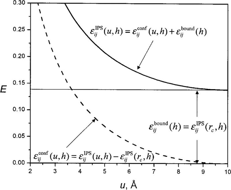
The IPS interaction as a function of the isotropic distance. At the cutoff boundary u = r_c = 10 Å, ε^IPS(r_c, h) ≠ 0. The IPS energy is divided into a boundary energy, ε^bound(h) = ε^IPS(r_c, h), and a configuration energy, ε^conf(u, h) = ε^IPS(u, h) – ε^IPS(r_c, h).

We divide the IPS energy into two parts, a configuration energy and a boundary energy (see Fig. 4):

$${\epsilon }_{ij}^{\text{IPS}}(u_{ij},h_{ij})={\epsilon }_{ij}^{\text{conf}}(u_{ij},h_{ij})+{\epsilon }_{ij}^{\text{bound}}(h_{ij}).$$ (40)

The configuration energy, ${\epsilon }_{ij}^{\text{conf}}(u_{ij},h_{ij})={\epsilon }_{ij}^{\text{IPS}}(u_{ij},h_{ij})-{\epsilon }_{ij}^{\text{IPS}}(r_c,h_{ij})$, is distance dependent, which approaches zero when u_ij → r_c. The boundary energy, ${\epsilon }_{ij}^{\text{bound}}(h_{ij})={\epsilon }_{ij}^{\text{IPS}}(r_c,h_{ij})$, is the energy at the boundary, which is independent of the isotropic distance. Correspondingly, the total energy of a system is also divided into a total configuration energy and a total boundary energy

$$\begin{gathered} E=\frac{1}{2}\sum _i^N\sum _j^{u_{ij}<r_c}{\epsilon }_{ij}^{\text{IPS}}(u_{ij},h_{ij}) \\ =\frac{1}{2}\sum _i^N\sum _j^{u_{ij}<r_c}{\epsilon }_{ij}^{\text{conf}}(u_{ij},h_{ij})+\frac{1}{2}\sum _i^N\sum _j^{u_{ij}<r_c}{\epsilon }_{ij}^{\text{bound}}(h_{ij}) \\ =E^{\text{conf}}+E^{\text{bound}}. \end{gathered}$$ (41)

The total configuration energy, which is continuous upon particles moving in and out of a local region, depends on the configuration of the local region:

$$E^{\text{conf}}=\frac{1}{2}\sum _i^N\sum _j^{u_{ij}<r_c}{\epsilon }_{ij}^{\text{conf}}(u_{ij},h_{ij}).$$ (42)

The total boundary energy depends on the number of particles in the local region and, for enclosed homogeneous systems, depends on the system volume and composition:

$$E^{\text{bound}}=\frac{1}{2}\sum _i^N\sum _j^{u_{ij}<r_c}{\epsilon }_{ij}^{\text{bound}}(h_{ij})\approx \frac{V_0}{2V}\sum _i^N\sum _j^N{\epsilon }_{ij}^{\text{bound}}(h_{ij}),$$ (43)

where V₀ and V are the volumes of the local region and the whole system, respectively. Equation (43) is based on the homogenous approximation that the number of particles in a local region is proportional to the volume of the local region. According to Eq. (43), E^bound depends on the volume of the local region and the particle densities of the whole system, while does not change upon particles moving in and out of a local region. Therefore, the total energy, Eq. (41), is continuous when particles cross local region boundaries.

For partially homogenous systems, when a particle is at the boundary of a local region, u_ij =r_c, the force in the isotropic direction is zero: $f_{uij}^{\text{IPS}}(r_c,h_{ij})=0$. Therefore, the force is continuous at the boundary in the isotropic direction. But in the anisotropic direction the force is not continuous because $f_{hij}^{\text{IPS}}(r_c,h_{ij})\ne 0$ (see Fig. 2). This difference in force continuity can be understood by the fact that there are periodic images in the isotropic direction but not in the anisotropic direction. Similar to the energy treatment, we can divide the IPS force into a configuration force and a boundary force:

$$\begin{gathered} f_{hij}^{\text{IPS}}(u_{ij},h_{ij})=[f_{hij}^{\text{IPS}}(u_{ij},h_{ij})-f_{hij}^{\text{IPS}}(r_c,h_{ij})]+f_{hij}^{\text{IPS}}(r_c,h_{ij}) \\ =f_{hij}^{\text{conf}}(u_{ij},h_{ij})+f_{hij}^{\text{found}}(h_{ij}). \end{gathered}$$ (44)

The total configuration force on particle i is

$$f_{hi}^{\text{conf}}=\sum _j^{u_{ij}>r_c}[f_{hij}^{\text{IPS}}(u_{ij},h_{ij})-f_{hij}^{\text{IPS}}(r_c,h_{ij})]$$ (45)

and the total boundary force is

$$f_{hi}^{\text{bound}}=\sum _j^{u_{ij}>r_c}{f}_{hij}^{\text{IPS}}(r_c,h_{ij})\approx \frac{V_0}{V}\sum _j^N{f}_{hij}^{\text{IPS}}(r_c,h_{ij}).$$ (46)

The configuration force is continuous at the boundary in all directions [$f_{hij}^{\text{conf}}(r_c,h_{ij})=0$ and $f_{uij}^{\text{conf}}(r_c,h_{ij})=f_{uij}^{\text{IPS}}(r_c,h_{ij})=0$]. Because the total boundary force shown in Eq. (46) is calculated in a way independent of the number of particles in local regions, the total force from Eq. (44) is continuous upon particles moving in and out of local regions.

For 3D homogenous systems things are simple. There is no boundary force and no anisotropic coordinate. The total electrostatic boundary energy can be simplified to

$$E_{\text{ele}}^{\text{bound}}=\frac{V_0}{2V}{\left(\sum _i^N{e}_i\right)}^2{\epsilon }_{\text{ele}}^{\text{IPS}}(r_c),$$ (47)

where e_i is the charge of particle i. Obviously, for neutral systems where ${\sum }_i^N{e}_i=0$, $E_{\text{ele}}^{\text{bound}}=0$. For the Lennard-Jones potential, the total boundary energy is

$$E_{L-J}^{\text{bound}}=\frac{V_0}{2V}\left({\epsilon }_{\text{rep}}^{\text{IPS}}(r_c)\sum _i^N\sum _j^N{A}_{ij}-{\epsilon }_{\text{disp}}^{\text{IPS}}(r_c)\sum _i^N\sum _j^N{C}_{ij}\right).$$ (48)

It should be noted that for molecular systems, all atom pairs, including self-pairs, must be considered when calculating configuration energies and configuration forces because all these pairs have been included in the calculation of the boundary energies and boundary forces in Eqs. (43), (45), (47), and (48). It is a normal practice that self-pairs and atoms forming bonds, bond angles, and dihedral angles are excluded or scaled down in a nonbonded energy calculation. Because the boundary energies are removed from all atom pairs, the configuration energies between all atom pairs, including self-pairs, should be calculated according to the following equation:

$${\epsilon }^{\text{conf}}(r_{ij})=\{\begin{array}{ll}{\varphi }_{ij}(u_{ij},h_{ij})-{\epsilon }_{ij}(r_c,h_{ij})-{\varphi }_{ij}(r_c,h_{ij})\hfill & 1-1,1-2,1-3\text{\hspace{1em}pairs}\hfill \\ {\epsilon }_{ij}^{(1-4)}(r_{ij})+{\varphi }_{ij}(u_{ij},h_{ij})-{\epsilon }_{ij}(r_c,h_{ij})-{\varphi }_{ij}(r_c,h_{ij})\hfill & 1-4\text{\hspace{1em}pairs}\hfill \\ {\epsilon }_{ij}(r_{ij})+{\varphi }_{ij}(u_{ij},h_{ij})-{\epsilon }_{ij}(r_c,h_{ij})-{\varphi }_{ij}(r_c,h_{ij})\hfill & \text{otherwise},\hfill \end{array}$$ (49)

where ${\epsilon }_{ij}^{(1-4)}(r_{ij})$ is a special energy function for 1–4 covalent bonded atom pairs, normally a function scaled down from ε_ij(r_ij). No exclusion or scale down should apply to ϕ_ij(u_ij, h_ij).

Pressure is an important property for simulation studies. When using IPS for energy calculation, the boundary energy must be considered accordingly for pressure calculation. Pressure is related to the partition function Q by the following equation:

$$\begin{gathered} P=-{\left(\frac{\partial A}{\partial V}\right)}_{NT}=-{\left(\frac{\partial A^{\text{id}}}{\partial V}\right)}_{NT}-{\left(\frac{\partial A^{\text{conf}}}{\partial V}\right)}_{NT}=\frac{NkT}{V} \\ +kT{\left(\frac{\partial \ln Q}{\partial V}\right)}_{NT}, \end{gathered}$$

where A^id is the Helmholtz free energy of idea gas and A^conf is the configuration contribution. After dividing the energy into the configuration energy and the boundary energy,

$$\begin{gathered} PV=NkT+\frac{VkT}{Q}\int \frac{\partial }{\partial V}{e}^{-E/kT}d\mathrm{\Omega }=NkT \\ -\frac{1}{Q}\int \left(V\frac{\partial E^{\text{conf}}}{\partial V}+V\frac{\partial E^{\text{bound}}}{\partial V}\right)e^{-E/kT}d\mathrm{\Omega }=NkT \\ +\langle W^{\text{conf}}\rangle +\langle W^{\text{bound}}\rangle . \end{gathered}$$ (50)

For 3D homogenous systems, the configuration viral W^conf can be calculated from interaction forces:

$$W^{\text{conf}}=-V\frac{\partial E^{\text{conf}}}{\partial V}=\frac{1}{6}\sum _i^N\sum _j^{r_{ij}<r_c}{r}_{ij}{f}_{ij}^{\text{IPS}}=\frac{1}{3}\sum _i^N{r}_i{f}_i^{\text{IPS}}.$$ (51)

The boundary viral W^bound can be derived from the boundary energy according to Eq. (43):

$$W^{\text{bound}}=-V\frac{\partial E^{\text{bound}}}{\partial V}\approx \frac{V_0}{2V}\sum _i^N\sum _j^N{\epsilon }_{ij}^{\text{IPS}}(r_c)=E^{\text{bound}}.$$ (52)

Similarly, when studying 2D or 1D homogenous systems, boundary energies also must be considered to calculate properties such as surface tension.

III. SIMULATION SYSTEMS AND CONDITIONS

We chose the following systems to examine the accuracy and application of the IPS method in long-range interaction calculations. The IPS energies are calculated using the third-order numerical function, Eq. (38), with parameters listed in Tables I, II, and III. The IPS method has been implemented into the CHARMM program⁶ and is available in version 32. The CHARMM force field²¹ is used in all calculations presented here.

A. CaCl² ionic fluids

This highly charged system is chosen to examine the calculation of electrostatic interactions. The ions interact through charge-charge Coulomb potential, Eq. (17), and the 6–12 Lennard-Jones potential, Eq. (21). There are 2048 Ca²⁺ ions and 4096 Cl⁻ ions in the system.

To generate homogenous conformations of different sizes, the system is simulated at a high temperature of 10 000 K to make the system fully expandable. During the simulations, the electrostatic interaction is calculated using the particle-mesh Ewald method,¹⁴ and the Lennard-Jones interaction is calculated with a force-switch cutoff method³ with a switch-on distance of 8 Å and a cutoff distance of 10 Å.

The conformations of a 1D homogenous system are generated by simulations in a 500 × 500 × L ų rectangular box, where L is the box side length in z axis with values varying from 60 to 160 Å. To keep the system together along the z axis, the 1D homogenous system is restrained with a cylinder potential of the form

$${\epsilon }_{1\text{D}}(r)=k(x^2+y^2).$$ (53)

The force constant is set to be k = 1 kcal/mol Ų. Figure 5(a) shows a typical conformation of the 1D homogenous system.

FIG. 5.

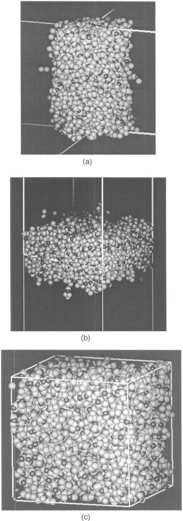
(a) A typical conformation of the 1D homogenous CaCl₂ system along z axis. (b) A typical conformation of the 2D homogenous CaCl₂ system along x–y plan. (c) A typical conformation of the 3D homogenous CaCl₂ system in a cubic box. The white lines mark the PBC boundaries. Ca²⁺ and Cl⁻ ions are represented by black and gray balls, respectively.

The conformations of a 2D homogenous system are generated by simulations in an L × L × 500ų rectangular box, where L is the box side length in x axis and y axis with values varying from 60 to 160 Å. To keep the system together along the x–y plane, the system is restrained with a planar potential function

$${\epsilon }_{2\text{D}}(r)=k{z}^2$$ (54)

The force constant is set to k = 1 kcal/mol Ų. Figure 5(b) shows a typical conformation of the 2D homogenous system.

The conformations of a 3D homogenous system are generated by simulations in an L × L × L ų cubic box with the box side length L ranging from 40 Å to 140 Å. Figure 5(c) shows a typical conformation of the 3D homogenous system.

B. Argon fluids

A cubic box of 9450 argon atoms is used to compare the calculation of Lennard-Jones interactions. Argon’s Lennard-Jones parameters [see Eq. (21)] are σ = 3.405 Å and ε₀ = −0.238 kcal/mol.

C. Acetylcholine binding protein and its pentamer

We chose the x-ray structures of acetylcholine binding protein (ACHBP) (Ref. 22) to examine the energy calculation for heterogeneous systems as well as the symmetry effect of periodic boundary conditions. The monomer and pentamer structures of this protein are shown in Fig. 6.

FIG. 6.

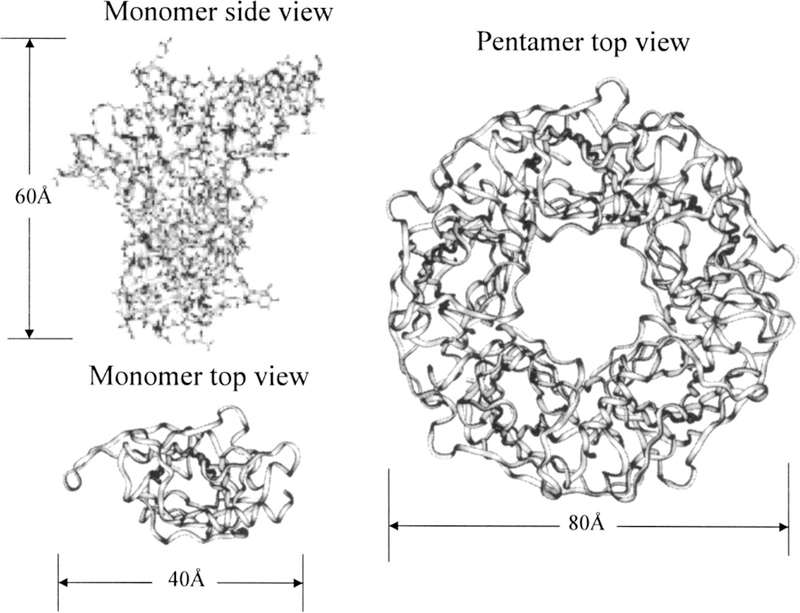
The x-ray structures of acetylcholine-binding protein (PDB code: li9b). The left images are the structure of its monomer viewed from side and top. The right image is a top view of the pentamer. The backbone traces are shown as ribbons. For clarity, atoms are rendered as sticks and are shown only in the side view of the monomer structure.

IV. RESULTS AND DISCUSSIONS

A. Comparison of long-range energy calculation methods

The IPS method introduces a distance-dependent image contribution to particle interactions. As a result, long-range interactions are transformed to short-range interactions as shown in Eq. (6). It would be interesting to examine how different the IPS interaction ε^IPS(r) is from the interactions calculated using other methods. Using the electrostatic potential, Eq. (17), as an example, we compare the IPS interactions with that from the cutoff methods, including straight truncation, energy switch, energy shift, force switch, and force shift,³ the reaction field method, as well as Ewald summation. The reaction field (RF) results are calculated using the Barker-Watts function:²³

$${\epsilon }^{\text{RF}}(r)=\frac{1}{r}+\frac{r^2}{r_c^3}\frac{ϵ-1}{2ϵ+1},$$ (55)

where ϵ is the predefined dielectric constant of the medium surrounding the local region.

Ewald summation results are calculated from the isotropic approximation functions, Eqs. (56) and (57), which are fitted to Ewald summation data with a simple cubic (SC) or a truncated octahedral (TO) periodic boundary condition by Adams and Dubey:²⁴

$$\begin{gathered} {\epsilon }_{\text{TO}}^{\text{Ewald}}(r)\approx \frac{1}{r}-\frac{3.36923345}{L}+\frac{3.53873}{L^3}{r}^2+\frac{8.33958}{L^5}{r}^4 \\ -\frac{28.51289}{L^7}{r}^6, \end{gathered}$$ (56)

$$\begin{gathered} {\epsilon }_{\text{SC}}^{\text{Ewald}}(r)\approx \frac{1}{r}-\frac{2.837297479}{L}+\frac{2.75022}{L^3}{r}^3 \\ -\frac{2.94414}{L^5}{r}^4+\frac{0.86910}{L^7}{r}^6. \end{gathered}$$ (57)

The IPS results are calculated using the following equation, which is derived from the third-order numerical function, Eqs. (38) and (39), with parameters shown in Table I:

$${\epsilon }^{\text{IPS}}(r)=\frac{1}{r}+\frac{2.737821}{r_c\sqrt{2}}+\frac{-2.737821+1.109466{\left(\frac{r}{r_c}\right)}^2+0.070800{\left(\frac{r}{r_c}\right)}^4+0.007918{\left(\frac{r}{r_c}\right)}^6}{\sqrt{2r_c^2-r^2}}.$$ (58)

The IPS method uses the radius of the local region, or the cutoff distance, r_c to define the local region, while Ewald summation uses lattice parameters (box sizes and angles) to define the local region. To make the two methods comparable, the local regions should have the same volume to produce images of the same densities. For the cubic box, this requires $L=\sqrt[3]{\frac{4}{3}\pi r_c^3}\approx 1.6120r_c$, and for the truncated octahedral box, this requires $L=\sqrt[3]{\frac{8}{3}\pi r_c^3}\approx 2.0310r_c$.

Figure 7(a) shows the electrostatic energies from different methods. The energies from the cutoff based methods are significantly lower than the Coulomb potential given by ε(r) = 1/r, because these methods assume zero energy beyond the cutoff distance. On the contrary, the IPS method, as well as the reaction field and Ewald summation, gives higher energies than the Coulomb potential.

FIG. 7.

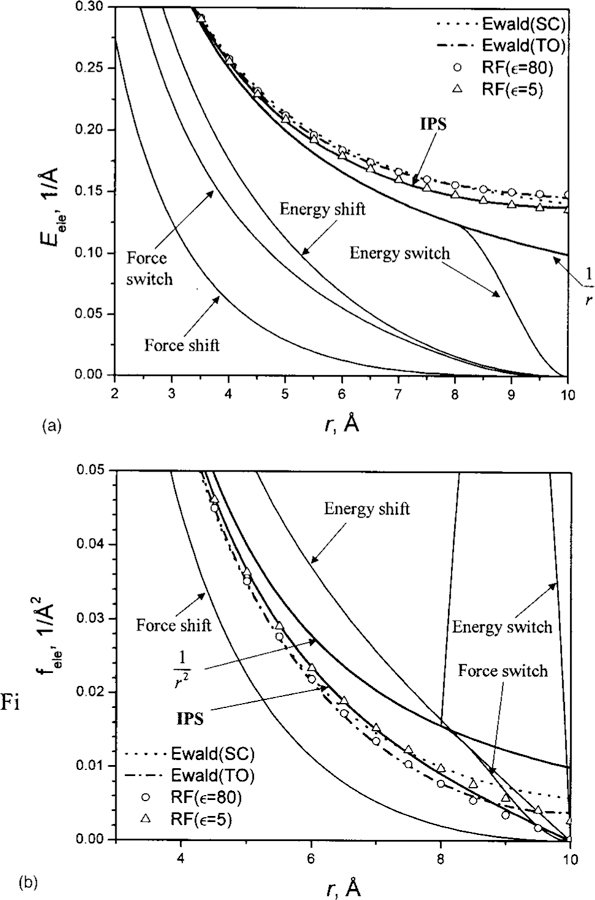
(a) The electrostatic energies calculated using different methods. (b) Electrostatic forces calculated from different methods. The cutoff distances for energy switch, energy shift, force switch, and force shift methods or the radius of local region for the IPS method are r_c = 10 Å. The force switch and energy switch are turned on at 8 Å. The reaction field (RF) results are calculated using Eq. (55). The Ewald results are calculated using Eq. (56) TO and Eq. (57) SC. The IPS results are calculated using Eq. (58). The box sizes for Ewald summation are set to be equal to the local region volume for the IPS calculation.

The reaction field results depend on the predefined dielectric constant ϵ. When ε = 1, the reaction field energies reduce to the Coulomb potential, ${\epsilon }_{ϵ=0}^{RF}(r)=1/r$. When ϵ = 5, the reaction field energies are very close to the IPS results, while at ϵ = 80, the reaction field energies are all above the IPS results. Overall, the IPS energies fall within the range of the reaction field results.

The Ewald energies are different in different periodic boundary conditions. In both cases, SC and TO, the Ewald energies are above the IPS results. Considering the fact that the Ewald isotropic approximations have maximum errors of 0.0097 Å⁻¹ for SC and 0.0062 Å⁻¹ for TO as compared to the true Ewald summation energies of this system,²⁴ we can say that the IPS energies are very close to the Ewald summation results.

Forces are more important than energies in molecular dynamics simulations. Figure 7(b) shows the forces calculated from different methods. As can be seen, except for the force-shift method, which produces much weaker forces than the IPS method, the cutoff-base methods produce stronger forces than the IPS method. The energy-switch method produces a very abrupt force in the switch region and should be used with great care. The reaction field forces show strong dependence on the predefined dielectric constant. At ϵ = 5, the reaction field forces agree with the IPS forces at short distances, while at ϵ = 80, a better agreement is found at distances close to the cutoff boundary. Compared with Ewald forces, the IPS forces are stronger at short distances, while at large distances the IPS force becomes weaker and is zero at the cutoff boundary.

Even though the reaction field method and the Ewald isotropic approximations produce energies and forces close to the IPS results, they are inconvenient to be applied directly to molecular dynamics simulations. For the reaction field method, the dielectric constant of the medium surrounding the local region must be predefined, which may cause artifacts in simulation results. Furthermore, if ϵ is not infinitely large, the force is not continuous at the cutoff boundary and additional shift or switch functions must be used, which may introduce additional artifacts to simulation results. For the Ewald isotropic approximations, first, they are different for different periodic boundary conditions. Second, they are approximations to the true Ewald summations and have large errors at large distances. Third, they do not have a defined boundary and normally are applied to all minimum images, which is time consuming for large systems. Also, their forces are not continuous when minimum images cross the periodic boundary. In all these aspects, the IPS method is a better solution.

B. Accuracy in calculating long-range interactions of homogeneous systems

For a homogeneous system of many particles, even though the IPS method and Ewald summation use different local regions and images, they should yield similar results if their local regions and images can correctly describe the homogenous system. Using different local regions and images should only cause differences in the partition between the local contribution and the long-range contribution as shown in Eq. (2), while the total interactions should remain the same.

Figure 8 shows the electrostatic energies of the highly charged CaCl₂ ionic fluid. The conformations are generated as a 3D homogenous system with different box sizes (the left panel). The energies from Ewald summation are compared with that from the cutoff method (the middle panel) and the IPS method (the right panel). A 10 Å cutoff is used for both the IPS method and the cutoff method. Because there are many ways to implement the cutoff method,³ to avoid any arbitrary factor, we chose straight truncation to perform the cutoff calculation in the following discussion. When the box size changes from 40 Å to 140 Å, the electrostatic energies change from −1.6 × 10⁶ kcal/mol to −1.3 × 10⁶ kcal/mol. The energies from the cutoff method show significant deviations from Ewald summation results, while the energies from the IPS method show very nice correlation with the Ewald results, indicating that the IPS method can be as good as Ewald summation in describing the electrostatic interactions. A comparison of forces calculated from different methods can be found in Fig. 12 and will be discussed later.

FIG. 8.

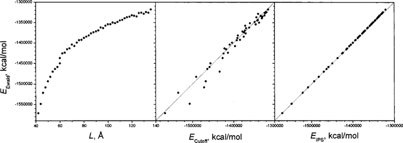
Electrostatic energies of the 3D homogenous CaCl₂ ionic fluid at conformations of different box sizes. The vertical axis is the energy calculated from Ewald summation. The left panel is against the box side lengths, the middle panel is against the energies calculated from the cutoff method with a cutoff distance of 10 Å, and the right panel is against the energies calculated from the IPS method with a local region radius of 10 Å.

FIG. 12.

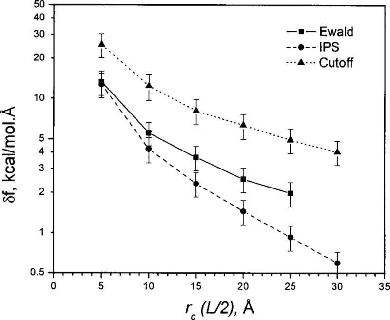
The rmsd of the electrostatic forces in a 3D homogenous CaCl₂ ionic fluid at different PBC box sizes for Ewald summation and at different cutoff distances for the IPS method and the cutoff method. The deviations are against the Ewald forces in a 60×60×60 ų PBC box. See text for details.

The accuracy of the IPS results increases with the size of the local region. Figure 9 shows the average deviations of the electrostatic energies using the cutoff and IPS methods at different cutoff distances. The energy deviations are calculated against the energies from Ewald summation. Clearly, the IPS method is one or two orders of magnitude more accurate than the cutoff method. As the cutoff distance increases, the accuracy of the IPS method increases nearly exponentially (linearly in the semilogarithm plot).

FIG. 9.

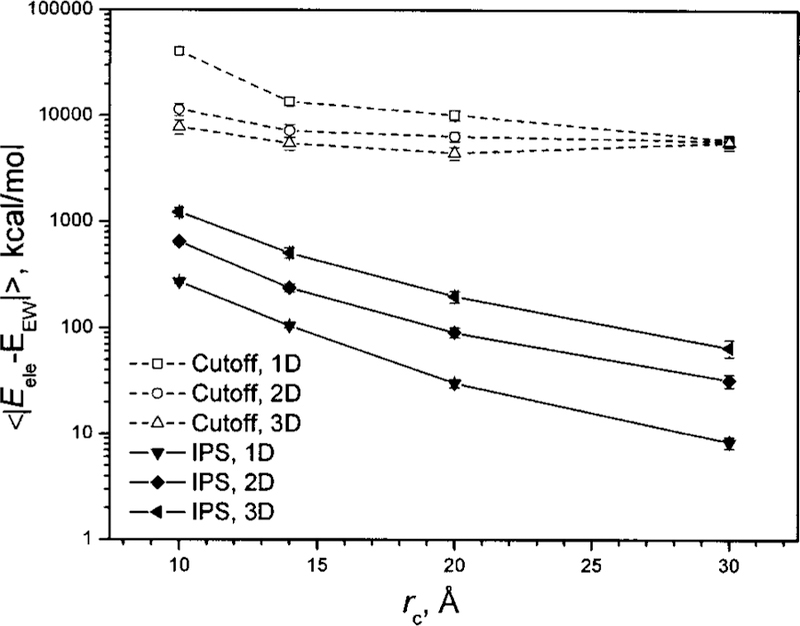
Average deviations of electrostatic energies calculated using the cutoff and IPS methods at different cutoff distances. The conformations of the CaCl₂ ionic fluid are generated as 1D, 2D, and 3D homogenous systems with different box sizes. The deviations are against the results of Ewald summation.

Figure 10 shows the accuracy of the Lennard-Jones energies calculated using the cutoff and IPS methods at different cutoff distances. Because the Lennard-Jones energy converges very quickly, we use the cutoff results with a 40 Å cutoff distance as the standard to calculate the deviations. As can be seen, the IPS method is significantly more accurate than the cutoff method for all types of homogenous systems. For 3D homogenous systems, the LRC method¹ can be used to improve the energy calculation. From Fig. 10 it is clear that the LRC substantially improves the accuracy, but not as much as does the IPS method. It should be stressed that LRC only improves energies, while IPS improves both energies and forces.

FIG. 10.

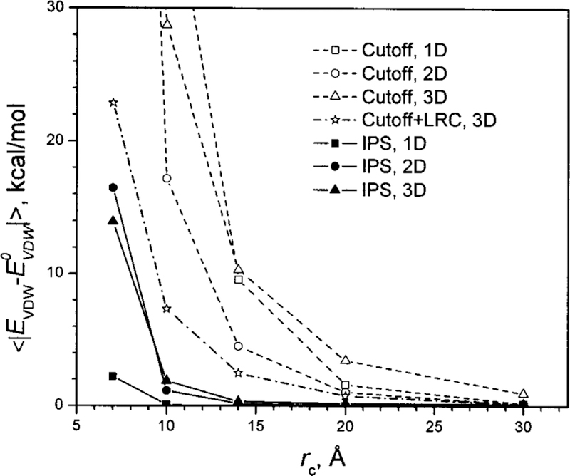
Average deviations of the Lennard-Jones energies calculated using the cutoff and IPS methods at different cutoff distances. The conformations of the CaCl₂ ionic fluid are generated as 1D, 2D, and 3D homogenous systems with different box sizes. The deviations are against the cutoff energies with a cutoff distance of 40 Å.

C. Accuracy in calculating long-range interactions of heterogeneous systems

Long-range interactions are also important in the study of large heterogeneous systems such as protein complexes. For large systems without periodic boundary conditions, the cutoff methods are the major approaches to calculate long-range interactions. It would be interesting to examine how well IPS can be applied to such heterogeneous systems.

We use the ACHBP monomer and pentamer shown in Fig. 6 to examine the accuracy of the IPS method. The size of the monomer is about 30 × 40 × 60 ų, while the size of the pentamer is about 60 × 80 × 80 ų. Using the forces calculated with no cutoff as the standard, we compare the rmsd of forces calculated with the cutoff method and the IPS method at different cutoff distances for the monomer and the pentamer (Fig. 11). As can be seen, for the monomer, the IPS method is more accurate when the cutoff distance is 12 Å or less, while for the pentamer, the IPS results are more accurate with cutoff distances up to 20 Å. These results indicate that when the a heterogeneous system is large as compared to the local region (the cutoff distance), it is better to assume isotropic periodic images than to assume a vacuum beyond the cutoff.

FIG. 11.

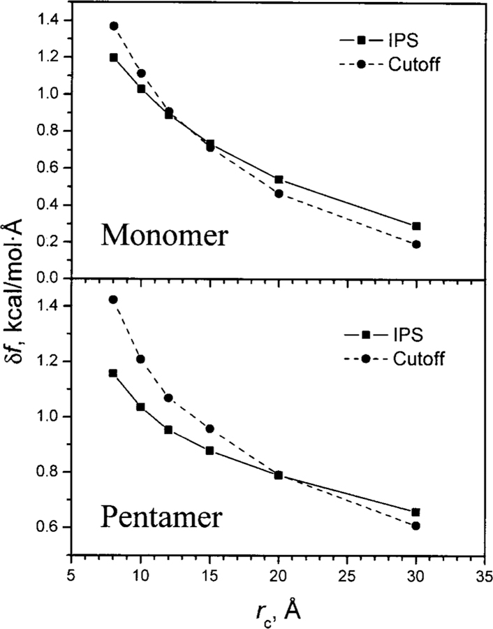
The root-mean-square deviations (rmsd) of the forces calculated from the cutoff method and the IPS method with different cutoff distances. The rmsd is calculated against the forces calculated with no cutoff. The monomer and pentamer structures of the acetylcholine-binding protein are shown in Fig. 6.

D. Comparison of lattice images and isotropic periodic images in describing long range interactions

Periodic boundary conditions are designed to overcome boundary effect. However, if the lattice images generated from periodic boundary conditions are used in energy calculation, the symmetry effect will be embedded into long-range interactions. Because periodic boundary conditions impose structural symmetries into a system and make it look like a super lattice, it is advised that the interaction range should not exceed the PBC box to minimize the imposed symmetry effect.¹ However, some long-range interactions such as the electrostatic potential extend far beyond a normal PBC box and a truncation at the box size will raise large errors. Therefore, using lattice images to calculate long-range interactions becomes a natural solution to get accurate interactions. Unlike lattice sum, the IPS method uses isotropic periodic images to calculate long-range interactions. It would be interesting to examine which images, the lattice images or the isotropic periodic images, can better describe long-range interactions.

As pointed out in Eq. (2), using images of any kind to represent long-range region is an approximation to a real system. The question is how accurate the interaction can be calculated with an image approximation. Here, we use a large box (60 × 60 × 60 ų) of the CaCl₂ ionic fluid under a cubic periodic boundary condition to represent a ‘‘real’’ system and the forces calculated in the large box system using Ewald summation are considered the ‘‘true’’ forces. For each ion, this system can be represented by a smaller local region (a cubic PBC cell) around it plus lattice images generated by the PBC. Also, this system can be represented by a spherical local region centered at the ion plus the isotropic periodic images around the local region. The particles in the local regions have the same configuration as in the large system, while the particles beyond the local region are replaced with either the lattice images for Ewald summation or the isotropic periodic images for the IPS method. The force deviation from the large system will measure how well these images describe long-range interactions.

Figure 12 shows the rmsd of forces calculated from Ewald summation with smaller PBC cells and from the IPS method as well as the cutoff method (straight truncation) at different cutoff distances. To be comparable, the Ewald results are plotted against the half box side length while the other methods against the cutoff distance. Clearly, the straight truncation method produces very inaccurate forces. The IPS forces are much more accurate than the cutoff forces, and the accuracy of the IPS forces increases nearly exponentially with the cutoff distances (linearly in the semilogarithm plot), similarly to the accuracy of the IPS energies (see Fig. 9). Interestingly, the forces from Ewald summation show larger rmsd than the IPS forces. Because the local regions have the same conformation as the real system, the force deviations come from the difference between the images and the real conformation beyond the local region. This result indicates that, with local regions of similar sizes, the lattice images results in larger force deviations than the isotropic periodic images. In other words, the isotropic periodic images can better describe long-range interactions than the lattice images.

The PBC symmetry effect is a serious problem when studying macromolecular systems. It is often the case that only one or several macromolecules of interest are included in a simulation system due to the limit in computing resources. The small number of macromolecules, which often account for a large portion of a system, make the system far from homogeneous and as a result, the periodic macromolecular system acts like a super lattice as shown in Fig. 13. Also due to the limit in computing resources, the box size is set as small as possible. The interaction between the macromolecule and its images will strongly depend on its orientation in the box, which could alter the conformational distribution.

FIG. 13.

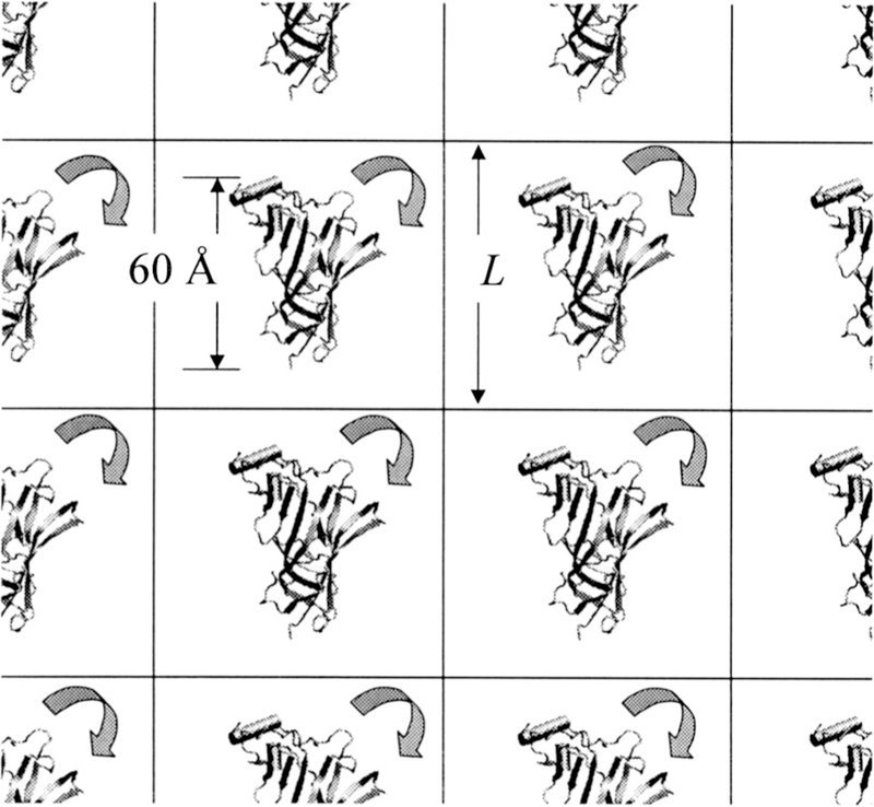
The ACHBP monomer under a cubic periodic boundary condition. Interactions with its images will depend on its orientation in the box and the size of the box.

We calculated the electrostatic energies of the system shown in Fig. 13 with different protein orientations using different methods. Figure 14 shows the energy ranges (the difference between the maximum and minimum energies over all orientations) at different box sizes. As can be seen, with Ewald summation, the energy range is more than 30 kcal/mol when the box size is 70 Å and is about 0.5 kcal/mol when the box size is as large as 160 Å. This orientational dependence of energy varies with protein conformations, and therefore, has strong effect on protein conformational distribution.

FIG. 14.

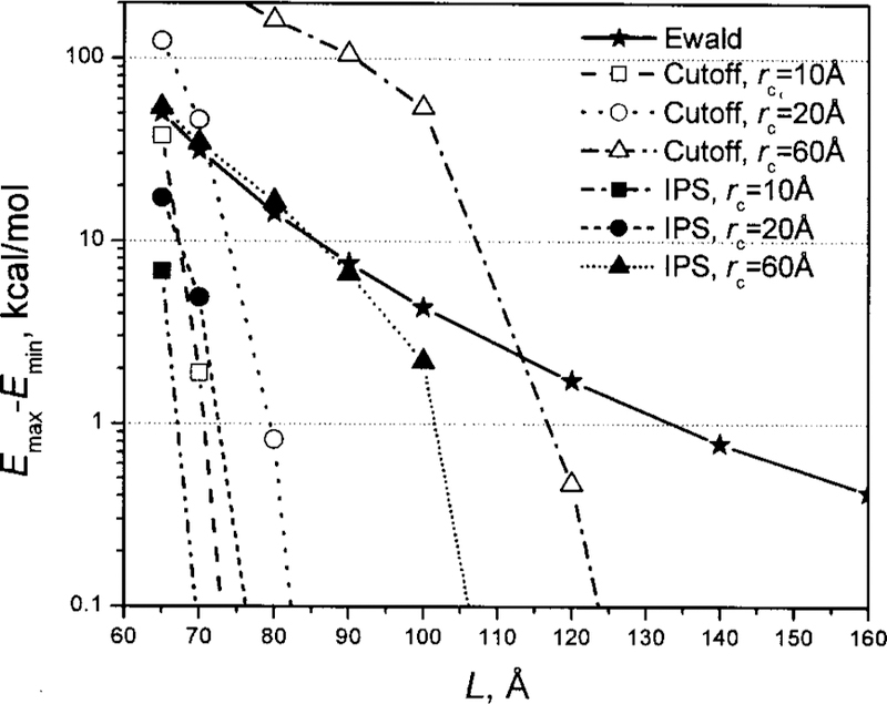
The orientational dependence of electrostatic energies at different box sizes. The system is shown in Fig. 13.

Using the cutoff method, the orientational dependence decays quickly as the box size increases. A smaller cutoff distance results in a quicker decay, because a smaller cutoff distance results in fewer images to be seen. When the cutoff distance is large as compared to the PBC box size, e.g., r_c = 60 Å for L<120 Å, the cutoff method has an even stronger orientational dependence than Ewald summation. That is the reason why the cutoff should not reach beyond a PBC box.

The IPS method shows an even smaller orientational dependence than the cutoff method and can eliminate orientational dependence with a PBC box: L> M + r_c, where M is the maximum molecular dimension and M ≈ 60 Å for this protein.

For macromolecular systems, the IPS method can fully consider the heterogeneity of a macromolecule by using a cutoff distance: r_c > M. When the cutoff distance is large compared to the PBC box size, e.g., r_c = 60 Å for L <100 Å, the IPS method shows orientational dependences similar to Ewald summation (Fig. 14). To eliminate the PBC symmetry effect while considering fully the heterogeneity of a macromolecule, a large PBC box, L ≈ 2 M, should be used.

E. Simulations using isotropic periodic sum

Molecular simulation can sample the energy surfaces of multibody systems and produce structural, thermodynamic, and dynamic properties of interest. Therefore, through simulations, we can examine how well overall the IPS describes the energy surface. Due to the space limit, we only present the following two examples.

The first example is to evaluate the description of long-range VDW interactions through N-P-T simulations of an argon fluid. The simulations are conducted at P = 1 atm and T = 100 K. Figure 15 shows the average densities and potential energies with different cutoff distances using three different methods, the cutoff method, the cutoff method plus LRC,¹ and the IPS method. The force-switch algorithm was used for the cutoff method.³ As can be seen (Fig. 15, the lower panel), using the cutoff method the density increases as the cutoff distance increases, indicating that a shorter cut-off distance results in more long-range interaction unaccounted. With LRC,¹ the dependence of the density on cutoff distances is much smaller but is still significant. Using the IPS method, the density is almost the same for all the cutoff distances from 8 Å to 40 Å. Similar behaviors are also found for the average potential energies shown in the upper panel of Fig. 15. These results clearly demonstrate that IPS can better describe long-range VDW interactions than the cutoff method, even augmented with LRC.

FIG. 15.

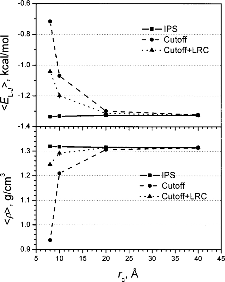
Average densities (lower panel) and average Lennard-Jones molar energies (upper panel) of the argon fluid from N-P-T simulations with different cutoff distances.

The second example is to evaluate the description of a charged system through N-V-T simulations of a highly charged ionic CaCl₂ fluid. The simulations are carried out at T = 10 000 K with a cubic PBC of 60×60×60 ų. The Lennard-Jones energies are calculated using the IPS method or the force-switch cutoff method plus LRC. The electrostatic energies are calculated using the IPS method, the force-switch cutoff method, or Ewald summation. Figure 16 shows the average Lennard-Jones energies (upper panel) and the average electrostatic energies (lower panel) from these simulations. As can be seen, the simulations using the cutoff method plus LRC show obvious dependence on cutoff distances in both average energies, while the simulations using the IPS method produce almost constant average energies with cutoff distances of 7 Å and up. The average electrostatic energies from the IPS simulations are almost identical to the simulation results using Ewald summation. These results clearly demonstrate that the IPS method can properly describe the energy surface of the system.

FIG. 16.

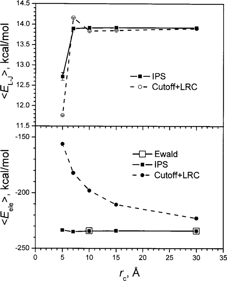
Average Lennard-Jones (upper panel) and electrostatic (lower panel) molar energies of the CaCl₂ ionic fluid from N-V-T simulations with different cutoff distances.

V. CONCLUSIONS

This work proposes an idea of using isotropic periodic images to describe statistically the remote structures of homogenous systems in the calculation of long-range interactions. The summation of interactions over isotropic periodic images is much easier than that over anisotropic lattice images used in lattice sum methods. This method can be applied to potentials of any functional form and for both fully and partially homogenous systems as well as finite systems. Analytic IPS functions of some typical potentials for fully (3D) homogenous systems are presented. For computing efficiency, we present a general numerical IPS function for potentials of the form: ε(r) = 1/rⁿ for both fully and partially homogenous systems.

For homogenous systems, the IPS method produces results very close to that from Ewald summation. The accuracy of IPS results increases exponentially with the cutoff distance. Through comparison with a large box of CaCl₂ ionic fluid, we demonstrate that the isotropic periodic images are better than lattice images in describing long-range interactions. For macromolecular systems, the IPS method is better than lattice sum methods by avoiding the symmetry effect imposed from periodic boundary conditions.

Like the cutoff methods, the IPS method can be applied to systems with or without periodic boundary conditions. For nonperiodic systems, the IPS method can better describe long-range interactions than the cutoff methods if the system size is large as compared to the cutoff distance. Because the IPS method is calculated the same way as the cutoff methods, it is comparable to the cutoff methods in computing cost and can be easily parallelized for multiprocessor computers.

References

- 1.Allen MP and Tildesley DJ, Computer Simulations of Liquids (Clarendon, Oxford, 1987). [Google Scholar]
- 2.Karplus M and Petsko GA, Nature (London) 347, 631 (1990). [DOI] [PubMed] [Google Scholar]
- 3.Steinbach PJ and Brooks BR, J. Comput. Chem 15, 667 (1994). [Google Scholar]
- 4.Brooks CL III, Pettitt BM, and Karplus M, J. Chem. Phys 83, 5897 (1985). [Google Scholar]
- 5.Kim KS, Chem. Phys. Lett 156, 261 (1989). [Google Scholar]
- 6.Brooks BR, Bruccoleri RE, Olafson BD, States DJ, Swaminathan S, Jaun B, and Karplus M, J. Comput. Chem 4, 187 (1983). [Google Scholar]
- 7.Baker JA and Watts RO, Mol. Phys 26, 789 (1973). [Google Scholar]
- 8.Tironi IG, Sperb R, Smith PE, and van Gusteren WF, J. Chem. Phys 102, 5451 (1995). [Google Scholar]
- 9.Hunenberger PH and van Gusteren WF, J. Chem. Phys 108, 6117 (1998). [Google Scholar]
- 10.Hummer G, Pratt LR, and Garcia AE, J. Chem. Phys 107, 9275 (1996). [Google Scholar]
- 11.Hummer G and Soumpasis DM, Phys. Rev. E 49, 591 (1994). [DOI] [PubMed] [Google Scholar]
- 12.de Leeuw SW, Perram JW, and Smith ER, Proc. R. Soc. London, Ser. A 373, 27 (1980). [Google Scholar]
- 13.Ewald PP, Ann. Phys. (Leipzig) 64, 253 (1921). [Google Scholar]
- 14.Darden T, York D, and Pedesen L, J. Chem. Phys 98, 10089 (1993). [Google Scholar]
- 15.Essmann U, Perera L, and Berkowitz ML, J. Chem. Phys 103, 8577 (1995). [Google Scholar]
- 16.Eastwood JW, Hockney RW, and Lawrence D, Comput. Phys. Commun 19, 215 (1980). [Google Scholar]
- 17.Greengard L, The Rapid Evaluation of Potential Fields in Particle Systems (MIT, Cambridge, MA, 1988). [Google Scholar]
- 18.Luty BA, Tironi IG, and van Gusteren WF, J. Chem. Phys 103, 3014 (1995). [Google Scholar]
- 19.Kurtovic Z, Marchi M, and Chandler D, Mol. Phys 78, 1155 (1993). [Google Scholar]
- 20.Lague P, Pastor RW, and Brooks BR, J. Phys. Chem. B 108, 363 (2004). [Google Scholar]
- 21.MacKerell AD Jr., Bashford D, Bellott M et al. , J. Phys. Chem. B 102, 3586 (1998). [DOI] [PubMed] [Google Scholar]
- 22.Brejc K, van Dijk WJ, Klaassen RV, Schuurmans M, van Der OJ, Smit AB, and Sixma TK, Nature (London) 411, 269 (2001). [DOI] [PubMed] [Google Scholar]
- 23.Baker JA and Watts RO, Mol. Phys 26, 789 (1973). [Google Scholar]
- 24.Adams DJ and Dubey GS, J. Comput. Phys 72, 156 (1987). [Google Scholar]