Mapping tissue water T ₁ in the liver using the MOLLI T ₁ method in the presence of fat, iron and B ₀ inhomogeneity

Abstract

Modified Look‐Locker inversion recovery (MOLLI) T ₁ mapping sequences can be useful in cardiac and liver tissue characterization, but determining underlying water T ₁ is confounded by iron, fat and frequency offsets. This article proposes an algorithm that provides an independent water MOLLI T ₁ (referred to as on‐resonance water T ₁) that would have been measured if a subject had no fat and normal iron, and imaging had been done on resonance. Fifteen NiCl₂‐doped agar phantoms with different peanut oil concentrations and 30 adults with various liver diseases, nineteen (63.3%) with liver steatosis, were scanned at 3 T using the shortened MOLLI (shMOLLI) T ₁ mapping, multiple‐echo spoiled gradient‐recalled echo and ¹H MR spectroscopy sequences. An algorithm based on Bloch equations was built in MATLAB, and water shMOLLI T ₁ values of both phantoms and human participants were determined. The quality of the algorithm's result was assessed by Pearson's correlation coefficient between shMOLLI T ₁ values and spectroscopically determined T ₁ values of the water, and by linear regression analysis. Correlation between shMOLLI and spectroscopy‐based T ₁ values increased, from r = 0.910 (P < 0.001) to r = 0.998 (P < 0.001) in phantoms and from r = 0.493 (for iron‐only correction; P = 0.005) to r = 0.771 (for iron, fat and off‐resonance correction; P < 0.001) in patients. Linear regression analysis revealed that the determined water shMOLLI T ₁ values in patients were independent of fat and iron. It can be concluded that determination of on‐resonance water (sh)MOLLI T ₁ independent of fat, iron and macroscopic field inhomogeneities was possible in phantoms and human subjects.

Abbreviations used

AMARES

advanced method for accurate, robust and efficient spectral fitting

bSSFP

balanced steady‐state free precession

ECF

extracellular fluid volume fraction

GRE

gradient recalled echo

HIC

hepatic iron concentration

MCSE

multiple contrast spin echo

MOLLI

modified Look‐Locker inversion recovery

NAFLD

non‐alcoholic fatty liver disease

PDFF

proton density fat fraction

shMOLLI

shortened MOLLI

STEAM

stimulated echo acquisition mode

TI

inversion time

TM

mixing time

1. INTRODUCTION

Quantifying the longitudinal relaxation time constant (T ₁) in clinical practice is often performed using the modified Look‐Locker inversion recovery (MOLLI) method1 or its variants,2, 3 due to their speed, precision, availability on clinical scanners and good reproducibility.4 This method has proved to be diagnostically useful both in cardiovascular MRI5 and in liver MRI, correlating with fibrosis and inflammation6 without the risks of biopsy.7 Liver T ₁ maps were also found to predict clinical outcomes in patients with chronic liver disease.8

However, T ₁ measured with MOLLI methods is sensitive not only to fibro‐inflammatory disease but also to a number of confounding factors that change the T ₁ or its measurement, either by altering the microscopic magnetic environment of the imaged tissue or by means of partial volume effects.

MOLLI and its variants generally employ a balanced steady‐state free precession (bSSFP) readout.1 The signal produced by bSSFP is dependent on the T ₁ and T ₂ of imaged proton species, flip angle and off‐resonance frequency.9 The frequency dependence, in particular, can result in complex behaviour of the bSSFP signal during T ₁ recovery when the imaged voxels contain both fat and water.10, 11, 12 With typical imaging parameters and clinically relevant fat fraction, this leads to an overestimation of the liver water MOLLI T ₁, at odds with the decrease expected in a simple partial volume model. This counterintuitive increase in MOLLI T ₁ with fat is in addition to the effect of iron deposits that reduce T ₁ and T ₂.13, 14 Magnetization transfer,15 heart rate,2 repetition time of the bSSFP readout10 and B ₀ inhomogeneity10 also influence MOLLI T ₁ values.

Removing the effect of iron on MOLLI T ₁ has previously been demonstrated,16 but to best characterize fibro‐inflammatory disease off‐resonance effects need to be removed, both B ₀ related and chemical shift related, to produce an on‐resonance water MOLLI T ₁. A disease where this might prove to be important is non‐alcoholic fatty liver disease (NAFLD), a condition characterized by hepatic lipid accumulation.17 NAFLD has a worldwide prevalence of 20–30%,18, 19 and encompasses a range of pathology from non‐alcoholic steatosis (simple fat accumulation) to non‐alcoholic steatohepatitis (fat accumulation associated with liver inflammation) to cirrhosis. In some cases, hepatocellular carcinoma may develop.20, 21 Since both the presence of fat and fibro‐inflammation cause MOLLI T ₁ values to increase at 3 T when using TR ≈ 2.3 ms, differentiating these two processes may provide additional insight into the disease and its progression.

The present study evaluates whether the confounding effect of lipids and off‐resonance frequency can be, in addition to the previous correction for the effect of iron, taken into account to provide a MOLLI T ₁ independent of the influence of these factors. Therefore, the target is a water MOLLI T ₁ value that would have been measured if a subject had no fat and normal iron, and imaging had been done on resonance.

2. METHODS

2.1. Phantom experiments

2.1.1. Construction

Fifteen agar‐based phantoms were built with varying proportions of fat and water. Phantoms were stored in 30 mL plastic sample containers (King Scientific, Huddersfield, UK) and were built in three batches, using a recipe similar to that described by Hines et al.22 To vary the T ₁ of water in each of the batches, NiCl₂ (Sigma‐Aldrich, St. Louis, MO, USA) solutions with concentrations of 0.45 mM, 0.73 mM and 1.61 mM were used. Next, 2%/weight agar (Sigma‐Aldrich), 0.01%/weight sodium benzoate (Sigma‐Aldrich), 43 mM sodium chloride (Sigma‐Aldrich) and 43 mM sodium dodecyl sulfate (Sigma‐Aldrich) were added. Each of the three solutions was boiled until it became transparent and viscous. Five sample containers were prepared for each batch, having 0%, 5%, 10%, 20% and 30%/vol. of peanut oil (Tesco, Welwyn Garden City, UK). Each container was filled to 30 mL with water‐agar solution. Each sample container was further homogenized for 5 min using an ultrasonic homogenizer (Eumax UD200SH, Hong Kong). The sodium dodecyl sulfate in the solution ensured that water and fat formed a homogenous emulsion. A 16th sample container was filled with 100% peanut oil. Peanut oil was chosen due to its ¹H spectrum resembling the ¹H spectrum of human subcutaneous fat.23

2.1.2. Imaging

Phantoms were scanned using a Siemens Tim Trio 3 T imager (Siemens Healthineers, Erlangen, Germany) equipped with a six‐channel body matrix coil (Siemens Healthineers) and a spine array coil (Siemens Healthineers) with 24 channels, of which nine were used. A set of multiple‐echo spoiled gradient recalled echo (GRE) images was collected to compute a map of the main magnetic field variation (γ ΔB ₀). Parameters of the 2D multiple‐echo GRE sequence were flip angle (FA) = 6°, TR/TE = 22.2/1.25, 2.46, 3.69, 4.92, 6.15, 7.38, 8.61, 9.84 ms, field of view (FOV) 302 × 245 mm², acquisition matrix 128 × 104, phase encoding direction anterior–posterior, BW = 1180 Hz/px, bipolar gradient readout scheme and slice thickness 7 mm. The map of γ ΔB ₀ field variation was determined from a T ₂*‐IDEAL fat‐water separation method with field map estimation using a graph‐cut algorithm.24, 25

T ₂ values of the fat‐free phantoms were determined using a multiple contrast spin echo (MCSE) experiment to quantify the effect of the agar and NiCl₂ on transverse relaxation. The following sequence parameters were used: TR/TE = 9000/15–480 ms in steps of 15 ms, FOV 270 × 270 mm², matrix 128 × 110, slice thickness 8 mm. Images with different contrasts were fitted to a mono‐exponential decay model. A MOLLI variant, shortened MOLLI (shMOLLI),2 was used to acquire a T ₁ map by collecting images at seven inversion times, over nine simulated heart beats with three inversions, using the 5(1)1(1)1 scheme, i.e. the first inversion pulse was followed by five readouts and a pause with a duration of one RR interval, the second inversion pulse was followed by one readout and a pause with a duration of one RR interval and the third inversion pulse was followed by one readout. ShMOLLI parameters followed a standardized protocol (Siemens WIP 561a, Erlangen, Germany): readout FA = 35°, TR/TE = 2.52/1.05 ms, FOV 290 × 343 mm², matrix 192 × 182, phase encoding direction anterior–posterior, BW = 898 Hz/px, slice thickness 8 mm, 28 lines before the central line, 82 total k‐space lines, shortest inversion time (TI) = 110 ms, inversion time increment 80 ms, generalized autocalibrating partially parallel acquisition (GRAPPA)26 acceleration factor 2 with 24 reference lines, partial Fourier factor 6/8 in the phase encoding direction and simulated heart rate of 60 beats/min. The approach to steady state was accelerated using five linearly increasing start‐up angle (LISA) pulses27, 28 and one half‐angle ramp down pulse. T ₁ values were obtained by applying the shMOLLI conditional fitting algorithm.2 All images were acquired in a coronal slice.

2.1.3. Spectroscopy

A set of ¹H spectra with multiple repetition times (TR) and echo times (TE) was collected using a multiple‐TR, multiple‐TE stimulated echo acquisition mode (STEAM) single‐voxel MRS sequence29 to characterize the T ₁ and T ₂ values of six fat peaks in the pure peanut oil phantom. Relaxation times of the pure peanut oil phantom were repeated at 20°C and 37°C. The multiple‐TR, multiple‐TE STEAM sequence followed the approach described by Hamilton et al.29: no water suppression, voxel size 14 × 14 × 24 mm³, mixing time (TM) = 9 ms, 24 spectra collected with TR varying between 150 and 2000 ms (150, 175, 200, 225, 250, 275, 300, 325, 350, 400, 450, 500, 600, 700, 800, 900, 1000, 1250, 1500, 2000 ms) and TE fixed at 15 ms, then eight spectra collected with a fixed TR of 1000 ms and TE changing from 20 to 110 ms (20, 25, 30, 35, 50, 70, 90, 110 ms). A version of the sequence with multiple TR but fixed TE = 15 ms was used to quantify individual T ₁ values of water and fat peaks in the mixed water and oil phantoms. Proton density fat fractions (PDFFs) were also determined from ¹H spectroscopy data. The obtained spectra were fitted using the MATLAB‐adapted version of the advanced method for accurate, robust and efficient spectral fitting (AMARES) algorithm,30, 31 and the resulting amplitudes for each peak were fitted to Equation 1, where S _0i is a scaling factor proportional to proton density, TE is the echo time, τ is the time from the third 90° pulse of the STEAM sequence to the end of the TR interval, i.e. the time during which the longitudinal magnetization recovery occurs, and i is an index for each spectral peak. Table 1 shows the prior knowledge used for the AMARES fitting.

$$S_i=S_{0i}\left(1-exp\left(-\frac{\tau }{T_{1i}}\right)\right)exp\left(-\frac{\mathrm{TE}}{T_{2i}}\right).$$ (1)

Table 1.

Prior knowledge of six fat peaks used to fit peanut oil spectra

Peak number	Chemical shift [ppm]	Line shape	Line width [Hz]	Peak name
1	0.90	Lorentzian	20	Methyl
2	1.30		40	Methylene
3	2.10		40	α‐carboxyl and α‐olefinic
4	2.76		20	Diacyl
5	4.30		40	Glycerol
6	5.30		30	Olefinic

When analysing multiple‐TR only experiments, the T _2i were fixed to be those determined in the pure peanut oil phantom and the 0% fat phantom. PDFF was defined as the ratio of the sum of observed fat proton densities and the sum of proton densities of water and observed fat peaks, as defined by Equation (2). Here $S_{0{\mathrm{f}}_i}$ denotes the proton density of the ith fat peak and S_0w is the proton density of water. These values were determined from fitting spectroscopy data to Equation 1.

$$\text{PDFF}\left[\%\right]=\frac{{\sum }_i{S}_{0{\mathrm{f}}_i}}{S_{0\mathrm{w}}+{\sum }_i{S}_{0{\mathrm{f}}_i}}\times 100.$$ (2)

2.1.4. Simulation

A Bloch equation simulation of the shMOLLI sequence was built in MATLAB (MathWorks, Natick, MA, USA). The simulation used the same parameters for the shMOLLI protocol as were used during the imaging experiments. The measured signal was determined as the average signal over 59 phase encode lines centred at k = 29. A hyperbolic secant 1 inversion pulse of 10.24 ms duration was used for inversion with time‐bandwidth product R = 5.48, peak B ₁ = 750 Hz and β = 3.45. The evolution of magnetization over time was simulated using Brian Hargreaves' Bloch equation simulator (http://mrsrl.stanford.edu/~brian/blochsim/).

Fat was characterized using the same six spectral peaks as evaluated by MRS. The chemical shift offset relative to water, relative amplitude and T ₁ and T ₂ relaxation times for each simulated component were determined from the multiple‐TR, multiple‐TE STEAM spectra of the peanut oil phantom.

As an initial test of the phantom model, three simulations of the water signal were carried out corresponding to the three NiCl₂ concentrations, using the water T ₂ values measured using the MCSE experiment and average STEAM water T ₁ values for the given NiCl₂ concentrations. The water and fat bSSFP signals were then combined according to the principle of partial volumes to reflect the PDFF determined from the multiple‐TR, multiple‐TE STEAM spectroscopy experiment for each fat‐water phantom and input to the shMOLLI T ₁ fitting algorithm. These simulated shMOLLI T ₁ values were then compared with the measured shMOLLI T ₁ as described in the statistics section.

2.1.5. Determining the water shMOLLI T ₁

To determine the shMOLLI T ₁ of the water component of the phantoms, the simulations above were repeated with water T ₁ varied over the 500–1600 ms range in steps of 1 ms, and the water and fat signals were again combined according to the measured PDFF. The simulated signal that satisfied the maximization problem described by Equation 3 was selected as the closest to the measured signal, where s represents simulated bSSFP signal vectors, s _meas is the measured bSSFP signal vector, θ is the angle between the simulated and measured signal,vectors and the numerator of the fraction represents the absolute value of the dot product of the two vectors while the denominator represents the product of the lengths of the two vectors).

$$s=\underset{s\in {ℂ}^7}{\text{argmax}}cos{\theta }_{s-s_{\text{meas}}}=\underset{s\in {ℂ}^7}{\text{argmax}}\frac{\mid s·s_{\text{meas}}\mid }{‖s‖·‖s_{\text{meas}}‖}.$$ (3)

Once the maximization was complete, an additional Bloch simulation was carried out to obtain the water‐only signal that would have been generated by the MOLLI sequence on resonance. This signal was then fitted to Equation 4 to determine the apparent T ₁ (T ₁*). ShMOLLI T ₁ was obtained using the imperfect32 Look‐Locker correction1, 32 as described by Equation 5.

$$S_{\mathrm{sim}}=A-Bexp\left(-\frac{TI}{T_1^{*}}\right)$$ (4)

$$T_1=T_1^{*}\left(\frac{B}{A}-1\right).$$ (5)

The T ₁ obtained in the last step was considered to be the water shMOLLI T ₁ value. This process was repeated for each of the phantom vials.

2.2. Patient study

2.2.1. Patient population

A total of 30 patients (18 female, mean age: 53 ± 8.3 years) with normal livers (N = 11), alcoholic liver disease (N = 1) and NAFLD (N = 18) were included. Participants were recruited from a hepatology clinic. Inclusion criteria were: adults aged between 18 and 75 years old, BMI between 25 and 50 kg/m², 1.5 ≤ ALT <10 ULN, blood pressure < 160/100 mm Hg and primary diagnosis of NAFLD. Exclusion criteria were: diagnosis of diabetes, blood haemoglobin <120 mg/dL, haemorrhagic disorders, anticoagulant treatment or presence of any contraindications to an MRI examination.

The study conformed to the ethical guidelines of the 1975 Declaration of Helsinki, and was approved by the institutional research departments and the National Research Ethics Service. All patients gave written informed consent.

2.2.2. Imaging

Patients were scanned using the same scanner and coils as described in the phantom work and using the same imaging and spectroscopic sequences. Six or nine channels of the spine array coil were used, depending on patient liver size.

T ₂* values were obtained using a T ₂*‐IDEAL fat‐water separation method with field map estimation using a graph‐cut algorithm and a signal model described by Hernando et al.25 (Equation 6).

$$S\left({\rho }_w,{\rho }_f,T_2^{*},{\mathit{TE}}_{\mathit{n}}\right)=e^{-\frac{{TE}_{\mathit{n}}}{T_2^{*}}}\left({\rho }_w+{\rho }_f\sum _{k=1}^P{\alpha }_k{e}^{2\mathit{\pi i}{f}_k{TE}_{\mathit{n}}}\right)e^{-2\mathit{\pi i\psi }{\mathit{TE}}_{\mathit{n}}}.$$ (6)

Here, ρ_w and ρ_f stand for the relative proton densities of water and fat, ψ represents field inhomogeneities, T ₂* is common for fat and water, TE_n represents the nth echo time, α _k is the relative amplitude of the kth fat peak, f _k is the chemical shift offset of the kth fat peak and p is the total number of fat peaks (p = 6 in our model). Equation 7 was then applied to obtain hepatic iron concentration (HIC) values in milligrams per gram dry weight of hepatic tissue.33, 34

$$\mathrm{HIC}\left[\mathrm{mg}/\mathrm{g}\mathrm{d}.\mathrm{w}.\right]=\frac{\left(\frac{1}{T_2^{*}}+11\right)}{2}\times 0.0254+0.202.$$ (7)

Hepatic shMOLLI T ₁ maps had TR = 2.45 ms, bSSFP TE varied between 1.02 and 1.05 ms, FOV was (270–300) × (360–400) mm², there were 24 k‐space lines before the central line and 66 total k‐space lines, the shortest inversion time was either 100 ms or 110 ms and the inversion time increment 80 ms.

Additionally, a single‐voxel long‐TR STEAM ¹H spectroscopy sequence35 was also run with and without water suppression. These spectra were used to quantify PDFF. Sequence parameters were the following: TR was cardiac gated and at least 2 s for suppressed spectra and at least 4 s for non‐suppressed spectra, TE = 10 ms and TM = 7 ms. Voxel size was 20 × 20 × 20 mm³ for both spectroscopy experiments. Water suppressed and non‐water‐suppressed spectra were processed using AMARES and combined with a specialized MATLAB script.35 When fat peaks were not visible, their amplitudes were determined using the relative amplitudes reported by Hamilton et al.36 PDFF was determined as the ratio of the sum of areas of fat peaks and the sum of water and fat peak areas, and was T ₂ corrected using Equation 8.

$$\mathit{\text{PDFF}}\left[\%\right]=\frac{{\sum }_i{F}_i}{W{e}^{\mathrm{TE}{R}_2}+{\sum }_i{F}_i}\times 100$$ (8)

where F _i are the fitted amplitudes of fat peaks, W is the fitted amplitude of the water peak, TE is the spectroscopic echo time and R ₂ is the transverse relaxation rate of the water in the liver in 1/s, given by Equation 9,33, 37, 38 where HIC is measured in mg/g dry weight.

$$R_2=\frac{1}{T_2}=\left(6.88+26.06{\left[\mathit{HIC}\right]}^{0.701}-0.438{\left[\mathit{HIC}\right]}^{1.402}\right)\times 1.47-2.2/\mathrm{s}.$$ (9)

All images were acquired in a single transverse slice positioned between the 10th and 11th thoracic vertebrae, during a breath‐hold. Breath‐held localized spectroscopy was performed in a voxel placed in the right lobe of the liver, away from the margin of the liver and from major blood vessels and bile ducts, making sure the voxel lay in the plane used for imaging. Breath‐hold lengths varied between 9 and 15 s for imaging and were 12 s for the long‐TR spectroscopy acquisition and 21 s for the multiple‐TR, multiple‐TE acquisition.

2.2.3. The MOLLI water T ₁ determination algorithm

Time‐varying magnetization of water and fat were simulated using Brian Hargreaves' Bloch equation simulator (http://mrsrl.stanford.edu/~brian/blochsim/). A version of the liver model introduced by Tunnicliffe et al.16 was used. This model comprises an intracellular and an extracellular space, with the extracellular space divided into an interstitial fluid pool and a blood pool in fast exchange. This liver model was extended with an additional fat component, and volume fractions of the extracellular fluid and the intracellular compartment were adjusted to reflect the fat fraction of the liver.

Exchange effects (both water exchange between intra‐ and extracellular spaces and magnetization transfer) were previously shown to have little influence on the simulation results,16 so the simulations presented here exclude exchange effects. Methods and results showing that exchange effects have little impact on these results can be found in the Supporting Information.

Fat was again characterized using six spectral peaks, with the chemical shift offsets relative to water and relative amplitudes given by Hamilton et al.36 T ₁ and T ₂ values of different lipid spectral peaks were fixed to values measured in the peanut oil spectra collected with the multiple‐TR, multiple‐TE STEAM sequence, except for the 2.76, 2.1, 1.3 and 0.9 ppm peaks of the human liver fat, for which T ₂ values reported by Hamilton et al.36 were used. T ₁ of the methylene fat peak at 1.3 ppm was quantified in patients with PDFF >5% using the multiple‐TR STEAM ¹H MRS sequence, and a value averaged over subjects was used in the simulations. Table 2 summarizes parameters used for the simulation.

Table 2.

Simulation parameters for the liver model at 3 T

Parameter	Value
PDFF	PDFF as measured by 1H STEAM MRS
v c	1 − vE − PDFF
v E	Simulated from 0.25 to (0.95 − PDFF)
v B	$\frac{1-v_{\mathrm{E}}-\text{PDFF}}{3}$
v I	vE − vB
f [Hz]	As determined from the multiple‐echo GRE sequence
Fat chemical shifts [ppm]	As determined from the multiple‐TR, multiple‐TE STEAM 1H MRS sequence of peanut oila
T 1fat [s]	T 1 of methylene peak determined from human 1H spectra. Others as determined from the multiple‐TR, multiple‐TE STEAM 1H MRS sequence of peanut oila
T 2fat [s]	Values taken from literature39 where available or from peanut oil spectraa
R 2E [1/s]	$\frac{3.64v_{\mathrm{B}}+2.9v_{\mathrm{I}}}{v_{\mathrm{E}}}+26.82\mathrm{HI}{\mathrm{C}}^{0.701}-0.451\mathrm{HI}{\mathrm{C}}^{1.402}$
R 2C [1/s]	11.0 + 46.0 HIC0.701 − 0.773 HIC1.402
R 1E [1/s]	$\frac{0.518v_{\mathrm{B}}+0.44v_{\mathrm{I}}}{v_{\mathrm{E}}}+0.029\mathrm{HIC}$
R 1C [1/s]	1.6 + 0.029 HIC

v _{(C, E, B, I)}, volume fractions of the intracellular pool, extracellular fluid, blood, and interstitial fluid; f, off‐resonance frequency. Both fat fraction and volume fractions are unitless. R _{2(E, C)}, transverse relaxation rates of extracellular fluid and intracellular pool; R _{1(E, C)}, longitudinal relaxation rates of extracellular fluid and intracellular pool.

^a For the full characterization of fat, see data in Table 3.

Longitudinal and transverse relaxation rates of non‐fatty compartments and their iron dependence were the same as described in the main simulation by Tunnicliffe et al.16 and are shown in Table 2. The longitudinal relaxation rate of the intracellular compartment in the absence of iron was determined such that the simulated signal for normal HIC (1.0 mg/g dry weight),16 0% fat, on resonance and normal extracellular fluid volume fraction (ECF) (0.4) had a fitted T ₁ value equal to the shMOLLI T ₁ in healthy volunteers of 717 ms.6

ECF was varied between 0.25 and (0.95 − PDFF) in steps of 0.01 and was used as a proxy for liver fibrosis. To have as good an approximation of the scanner measurement as possible, the shMOLLI RF pulse sequence was simulated using the exact inversion, repetition and echo times, as well as number of phase encoding lines, extracted from the patient shMOLLI images. Once separate bSSFP signals were simulated for the intracellular pool, extracellular pool and hepatic fat, they were combined as a volume fraction‐weighted sum, as given by

$$S_{\mathrm{sim}}=\left(\mathrm{ECF}{S}_{\mathrm{e}}+\left(1-\mathrm{ECF}{S}_{\mathrm{i}}\right)\right)\left(1-\text{PDFF}\right)+\text{PDFF}{S}_{\mathrm{f}}.$$ (10)

In this equation S _sim represents the overall simulated shMOLLI signal, S _e is the simulated extracellular signal, S _i is the simulated intracellular signal and S _f is the simulated fat signal.

As before, the optimal simulated signal was identified via the maximization problem described by Equation 3. An ROI was placed in the posterior or lateral parts of the right lobe, in such a way as to avoid vessels and bile ducts and as close as possible to the spectroscopy voxel. The ECF corresponding to the optimal signal was used to simulate a fat‐ and iron‐free signal on resonance and T ₁ and T ₂ values of the liver compartments corresponding to normal HIC. This signal was then processed using the shMOLLI conditional fitting algorithm to obtain a water shMOLLI T ₁ which should be independent of iron, fat and off‐resonance frequency.

In addition, in two subjects, three separate shMOLLI T ₁ maps were produced for a single liver slice: an iron‐corrected, on‐resonance water shMOLLI T ₁ (using the full processing described in the paragraph above); iron‐corrected, on resonance mixed fat‐water shMOLLI T ₁; and iron‐corrected, inhomogeneous B ₀, water shMOLLI T ₁. Voxel‐by‐voxel PDFF values were determined from the T ₂*‐IDEAL fat‐water separation method described above followed by a magnitude‐based IDEAL algorithm.40 For one of the participants the shMOLLI T ₁ map and GRE data used for this experiment were collected after a linear frequency change was induced in the right–left direction by changing the value of the shim gradient in the x direction.

The mechanisms used for both phantom and patient on‐resonance water MOLLI T ₁ are summarized in a block diagram shown in Figure 1.

Figure 1.

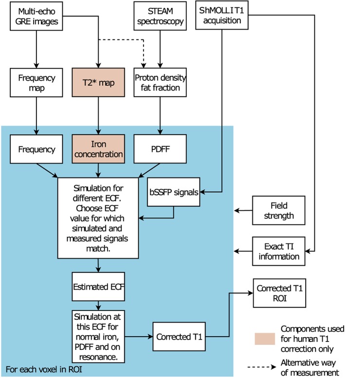
Block diagram of the water shMOLLI T ₁ determination algorithm. In addition to the shMOLLI T ₁ map, a multiple‐echo GRE image set and a STEAM ¹H spectrum were also collected to derive a B ₀ field map of the imaged slice and the PDFF. When the algorithm was used to determine water shMOLLI T ₁ values in patients, the GRE images were also used to generate T ₂* values and thus HIC values. Knowledge of field strength was necessary for the correct modelling of lipid peaks and the effects of iron. The actual (heart‐rate‐dependent) inversion times were used as in the imaging experiments to eliminate possible errors caused by variable heart rates2

The liver model was verified against a forward simulation of patient shMOLLI T ₁ measurements by simulating the extracellular, intracellular and fat bSSFP signals. The extracellular volume fraction for each patient was estimated based on the spectroscopically measured water T ₁ and using the relationship between blood volume fraction and interstitial volume fraction as given in Table 2 and given T ₁ of intra‐ and extracellular compartments. T ₁ and T ₂ for the simulations were determined based on Table 2 for the intracellular and extracellular compartments, given the patient's measured HIC. The fat signal was simulated using the T ₁ and T ₂ values in Table 3. These simulated signals were combined as a volume‐fraction weighted sum and fit using the shMOLLI algorithm to produce the expected shMOLLI T ₁ given this measured spectroscopic T ₁.

Table 3.

Fat peak parameters used in the Bloch simulation of the shMOLLI sequence. T ₁ and T ₂ values of fat peaks in peanut oil were measured at room temperature (20°C) for the phantom work and at human body temperature (37°C) for human experiments

			Peanut oil (T = 20°C)		Participants (T = 37°C)
Peak number	Chemical shift (relative to tetramethylsilane) [ppm]	Relative amplitude [a.u.]	T 1 ± SD [ms]	T 2 ± SD [ms]	T 1 ± SD [ms]	T 2 ± SD [ms]
1	0.90	0.087	264 ± 20	54 ± 3	333 ± 12a	83b
2	1.30	0.693	291 ± 21	61 ± 1	312 ± 17c	62b
3	2.10	0.128	231 ± 18	52 ± 3	254 ± 8a	52b
4	2.76	0.004	248 ± 25	61 ± 5	273 ± 8a	51b
5	4.30	0.039	193 ± 14	43 ± 2	228 ± 8a	49 ± 3a
6	5.30	0.049	285 ± 15	48 ± 2	332 ± 15a	50 ± 4a

^aAs measured in peanut oil.

^bAs reported by Hamilton et al.36

^cAs measured in livers of participants.

2.3. Statistical analysis

Correlation between simulated and measured shMOLLI T ₁ values of phantoms, as well as correlation of iron‐corrected shMOLLI T ₁ and iron‐, fat‐ and off‐resonance‐independent water shMOLLI T ₁ values with spectroscopically determined water T ₁ values in patients, was evaluated using Pearson's correlation coefficient. Bland–Altman plots41 were built to evaluate agreement between water T ₁ values derived from STEAM spectroscopy and iron‐corrected shMOLLI T ₁ values, and between water T ₁ values derived from STEAM spectroscopy and iron‐, fat‐ and off‐resonance‐independent water shMOLLI T ₁ values. A left‐tailed F‐test was used to evaluate the change in the variance of T ₁ differences shown on the Bland–Altman plots. All statistical hypothesis testing was performed at significance level α = 0.05.

3. RESULTS

3.1. Phantom experiments

Table 3 summarizes the results of measurements made using the 100% peanut oil phantom. These values were used to characterize fat in the phantom correction algorithm.

Table 4 shows PDFF, T ₁, T ₂ and shMOLLI T ₁ of individual fat‐water phantoms. Simulated and measured phantom shMOLLI T ₁ values showed good agreement (r = 0.999, P < 0.001), as reflected by Figure 2A. Figure 2B shows the corrected on‐resonance water shMOLLI T ₁ in comparison with the measured shMOLLI T ₁ values. Fat‐dependent shMOLLI T ₁ had a clear systematic dependence on PDFF and a weaker correlation (r = 0.910, P < 0.001) with spectroscopy‐based T ₁ than fat‐independent water shMOLLI T ₁ (r = 0.998, P < 0.001). On‐resonance water shMOLLI T ₁ had significantly (F = 15.003, P = 0.0046) lower variance than measured shMOLLI T ₁ of the difference between phantom water T ₁ values measured by STEAM and by shMOLLI, as shown in Figure 3.

Table 4.

Baseline parameter values for fat‐water phantoms, as measured with multiple‐contrast spin echo, shMOLLI and multiple‐TR STEAM ¹H MRS. Water T ₂ and shMOLLI T ₁ were averaged over circular regions of interest on corresponding maps

NiCl 2 concentration [mM]	PDFF [%]	STEAM T 1 of water ± SD [ms]	T 2 of water ± SD [ms]	shMOLLI T 1 ± SD [ms]
0.45	0.0	1390 ± 30	78 ± 3	1294 ± 31
	7.0	1386 ± 24	a	1340 ± 29
	10.3	1425 ± 35	a	1433 ± 38
	15.6	1392 ± 29	a	1527 ± 42
	26.8	1386 ± 17	a	1736 ± 62
0.73	0.0	1148 ± 29	82 ± 2	1071 ± 18
	7.3	1177 ± 34	a	1132 ± 25
	11.1	1169 ± 20	a	1156 ± 21
	16.0	1136 ± 30	a	1236 ± 31
	24.7	1135 ± 28	a	1303 ± 39
1.61	0.0	690 ± 23	89 ± 5	627 ± 7
	6.8	690 ± 29	a	651 ± 7
	12.6	689 ± 27	a	680 ± 8
	21.5	684 ± 20	a	735 ± 11
	27.0	687 ± 16	a	798 ± 12

^aAs the MCSE experiment could not be used to determine water T ₂ when mixed with fat, we have used the same water T ₂ within a NiCl₂ concentration group as the T ₂ measured in the 0% fat phantom of each group.

Figure 2.

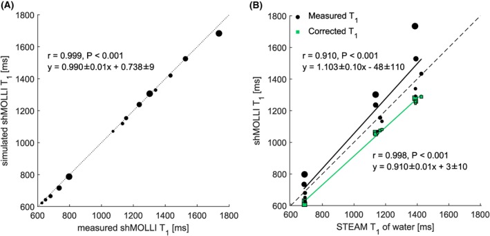
A, “Forward” shMOLLI simulation of the phantoms shows excellent agreement with measured shMOLLI T ₁ values. B, Correlation between shMOLLI T ₁ and spectroscopy‐based T ₁ increases after removing the effects of fat. It is expected to obtain shMOLLI T ₁ values lower than those obtained from spectroscopy after the determination of water shMOLLI T ₁ values.32 Points on both graphs are size‐coded as a function of phantom PDFF

Figure 3.

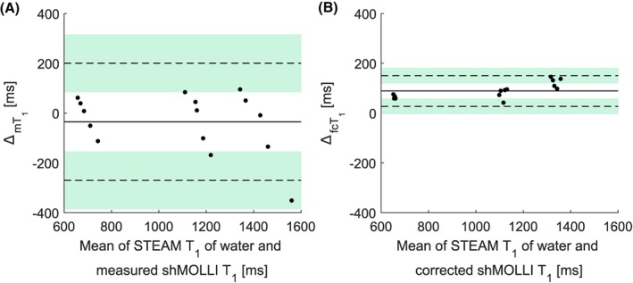
Bland–Altman plots showing phantom data before (A) and after (B) applying the water shMOLLI T ₁ determination algorithm. The near‐zero bias in A is due to the increased shMOLLI T ₁ values observed at high fat fractions, while a bias of 89 ms in B can be explained by the expected2 underestimation of T ₁ values by the shMOLLI method. An F‐test performed on the two differences shown in A and B revealed that the variance of the measurements was statistically significantly decreased after removing the effects of fat, iron and off‐resonance frequency (F = 15.003, P < 0.001). ${\Delta }_{\mathrm{m}{T}_1}$ is the difference between STEAM T ₁ and the measured shMOLLI T ₁; ${\Delta }_{\mathrm{fc}{T}_1}$ is the difference between STEAM T ₁ and the fat‐independent water shMOLLI T ₁

3.2. Patient studies

Of 30 patients, 19 (63.3%) had hepatic steatosis (PDFF >5%). The patients' fat fractions ranged from 1.53% to 20.33% and T ₂* values ranged from 6.3 ms to 37.9 ms (HIC range 0.6768 mg/g dry weight‐2.357 mg/g dry weight). Figure 4A shows the results of the forward simulation, while Figure 4B shows the results of the fat correction in patients. While iron‐corrected shMOLLI T ₁ values correlated moderately (r = 0.493, P = 0.005) with spectroscopically measured water T ₁ values, the fat‐independent water shMOLLI T ₁ determination algorithm yielded a stronger correlation with STEAM T ₁ values (r = 0.771, P < 0.001). Similarly, the large variability between STEAM and iron‐corrected shMOLLI T ₁ introduced by the effect of fat is significantly reduced by the water shMOLLI T ₁ determination algorithm (F = 0.3448, P = 0.0023), as seen in Figure 5B.

Figure 4.

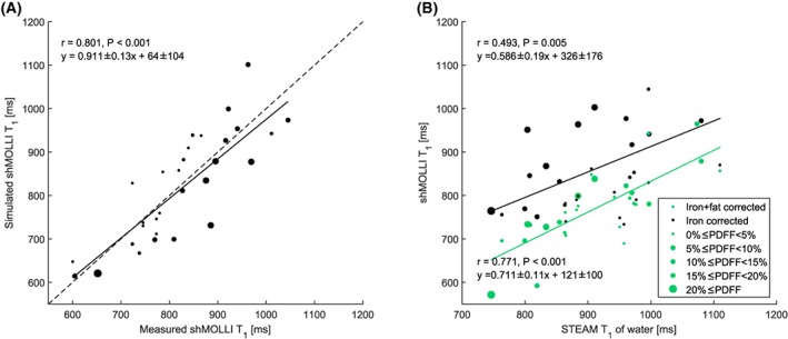
A, “Forward” simulation of patient shMOLLI T ₁ measurements. B, Correlation between water shMOLLI T ₁ values and spectroscopically measured T ₁ of the water in the liver increased after extending the initial iron‐only correction to remove the effects of iron, fat and off‐resonance

Figure 5.

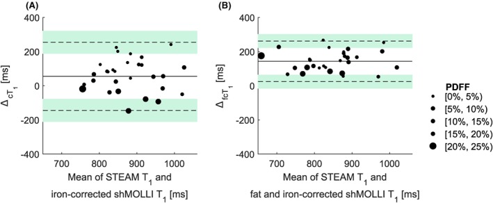
Bland–Altman plots of the iron‐corrected (A) and iron‐, fat‐ and off‐resonance‐independent (B) patient data reveal a statistically significant (F = 0.3448, p = 0.0023) reduction of the variance in the difference between STEAM T ₁ and shMOLLI T ₁ values after removing the effects of iron, fat and B ₀ inhomogeneities and remove the systematic trend for higher fat to give higher shMOLLI T ₁. As in the case of phantoms, the large bias in B is caused by the previously shown2 underestimation of T ₁ values by the shMOLLI method. ${\Delta }_{c{T}_1}$ is the difference between the STEAM T ₁ of the water in the liver and the iron‐corrected shMOLLI T ₁; ${\Delta }_{\mathit{fc}{T}_1}$ is the difference between the STEAM T ₁ of the water in the liver and the iron‐, fat‐ and off‐resonance‐independent water shMOLLI T ₁

Relaxation times of individual fat peaks used for modelling the fat compartment are summarized in Table 3.

Table 5 contains linear regression coefficients for the dependence of shMOLLI T ₁ on water STEAM T ₁, PDFF and R ₂* (=1/T ₂*) values as well as P‐values associated with these coefficients, showing that on‐resonance water shMOLLI T ₁ values do not show statistically significant dependence on fat.

Table 5.

Linear regression correlation coefficients for shMOLLI T ₁ dependence on water STEAM T ₁, PDFF and liver R ₂*, determined from original measured shMOLLI T ₁ values, iron‐corrected shMOLLI T ₁ values, and iron‐, fat‐, and off‐resonance‐independent water shMOLLI T ₁ values. Coefficients are shown as estimate ± standard error

	STEAM T 1 coefficient [ms shMOLLI T 1 /ms STEAM T 1 ]	P‐value	PDFF coefficient [ms shMOLLI T 1 /% PDFF]	P‐value	R 2 * coefficient [ms shMOLLI T 1 /(1/s) R 2 *]	P‐value
Measured shMOLLI T 1	0.5 ± 0.2	0.0051	11.7 ± 2.5	< 0.0010	−1.7 ± 0.4	<0.0010
Iron‐corrected shMOLLI T 1	0.8 ± 0.1	<0.0010	13.9 ± 2.1	< 0.0010	−0.4 ± 0.4	0.3544
Iron‐, fat‐ and off‐resonance‐independent water shMOLLI T 1	0.7 ± 0.1	<0.0010	2.9 ± 1.7	0.1040	−0.6 ± 0.3	0.0400

Figure 6 shows the results of applying the algorithm pixel by pixel over a single‐slice liver shMOLLI T ₁ map of two patients. The liver in the right‐hand column had, on average, HIC = 1.16 mg/g dry weight, PDFF = 15.83% and a linearly varying frequency offset in the left–right direction with frequency offsets ranging from −50 Hz to 35 Hz, which was artificially applied by manually modifying the B ₀ shim. The liver in the left column had an average HIC = 2.69 mg/g dry weight and PDFF = 8.35%.

Figure 6.

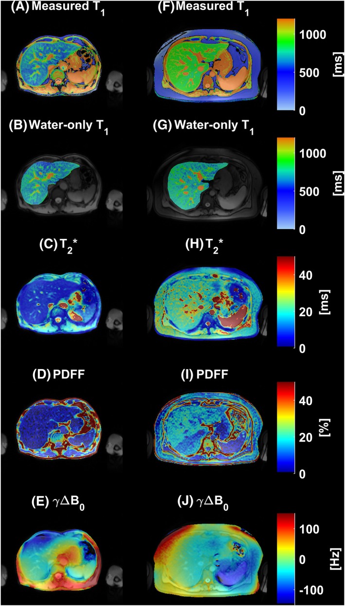
A, F, Two examples of liver shMOLLI T ₁ maps affected by iron, fat and B ₀ inhomogeneity. B, G, Normal liver T ₁ maps resulted after removing the effects of fat, iron and B ₀ inhomogeneity. C, H, The calculated T ₂* maps show a homogeneous distribution of increased (mean HIC = 2.69 mg/g dry weight) (C) and normal iron concentrations (mean HIC = 1.16 mg/g dry weight) (H). D, E, I, J, Full PDFF (D, mean PDFF = 8.35%; I, mean PDFF = 15.83%) and B ₀ field maps (E, mean γ ΔB₀ = 1.78 Hz; J, mean γ ΔB₀ = −8.81 Hz) are also shown

The different effects on the overall on‐resonance water‐only T ₁ determination are shown in Figure 7 for the participant who had the x shim manually changed over the liver. Figures 7B, 7C and 7D show the results of the algorithm with three different models applied on the same T ₁ map of the liver: full modelling of the effects of iron, fat and B ₀ inhomogeneity (Figure 7B), a model of iron and fat effects (Figure 7C) and a model containing effects from iron and B ₀ inhomogeneity (Figure 7D). The maps in the second row of Figure 7 show the T ₁ difference between the complete model and the partial models. As expected, a linear variation in off‐resonance frequencies over a range including both positive and negative values caused both an increase and a decrease of T ₁ values,10 in this case by up to 50 ms. This under‐ and overestimation of T ₁ values is reflected in the difference between the iron‐, fat‐ and off‐resonance‐independent water shMOLLI T ₁ map and the iron‐ and fat‐independent T ₁ map of Figure 7E. When removing the effects of iron and off‐resonance frequencies only, the effects of fat lead to higher‐than‐expected shMOLLI T ₁ values, as shown in Figure 7F, in this case by up to 250 ms.

Figure 7.

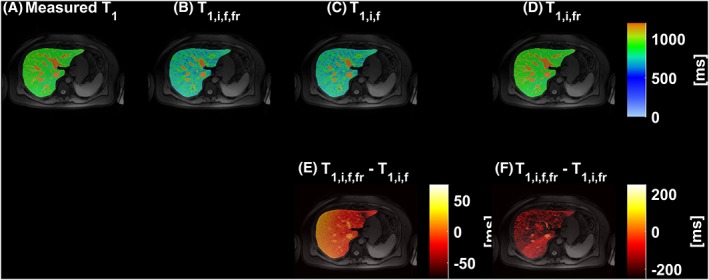
Three models were used in total to determine water‐only shMOLLI T ₁ based on a measured shMOLLI T ₁ map (A). In addition to the full model of iron, fat and off‐resonance effects (B), two additional models were implemented: one without accounting for B ₀ inhomogeneity and another without accounting for fat. C, The resulting T ₁ map after the effects of iron and fat have been removed; E, the difference between the T ₁ map obtained by using the full model and this alternative corrected T ₁ map. D, Removing the effects of iron and B ₀ inhomogeneity only yields higher‐than‐normal T ₁ values. The difference between this alternative T ₁ map and the water shMOLLI T ₁ map determined using the full model (F) is explained by the effects of the fat

4. DISCUSSION

This study describes an extension of the liver model proposed by Tunnicliffe et al.16 to include a variable sized fat compartment and a frequency offset calculated from the GRE data used for T ₂* mapping, thus obtaining a model reflecting the effects of iron, fat and off‐resonance frequencies on T ₁ measured by MOLLI variants. This model then allowed the identification of an on‐resonance water shMOLLI T ₁ value: the value that would have been measured if subjects had 0% PDFF, and normal HIC (i.e. 1 mg/g dry weight) and were imaged in a perfectly homogeneous static magnetic field. The results of the on‐resonance water shMOLLI T ₁ determination algorithm showed excellent correlation with spectroscopically determined water T ₁ values in phantoms, and increased statistically significant correlation in human participants, when compared with iron‐corrected shMOLLI T ₁, and reduced variance of the difference between STEAM T ₁ of water and water shMOLLI T ₁. While we report our results for the particular case of using the shMOLLI T ₁ mapping method, the water T ₁ determination algorithm is equally applicable to other variants of the MOLLI acquisition method, as long as the specific timing is included in the Bloch simulations..

In addition to the assumptions of Tunnicliffe et al. regarding the homogeneous distribution of iron between the liver parenchyma and extracellular fluid, we further assumed that fat droplets in hepatocytes appear in a macrovesicular form, which is mostly prevalent in NAFLD,42 thus not affecting the tumbling rate of water molecules in hepatocytes. We have not explored possible different relaxation mechanisms in the presence of microvesicular fat.

A further assumption was that the T ₁ and T ₂ relaxation times of lipid protons are independent of iron. It has been shown previously that the T ₂* of both water and fat is affected by iron.43 However, fat diffuses much more slowly than water molecules because of the high molecular weights of constituent triglycerides; therefore, their transverse T ₂ relaxation will be affected less by local field inhomogeneities. The independence of longitudinal relaxation of fat on iron is guaranteed by the lack of magnetization transfer between lipid macromolecules and water.44

In the T ₂*‐IDEAL model we assumed equal T ₂* values for fat and water to ensure numerical stability of the fitting. However, the T ₂* values of these two species might not be identical due to a susceptibility difference between them.45 Errors in fat quantification due to this simplification appear in Bydder et al45 to be small enough that they would not have caused substantial changes in our proposed water‐T ₁ determination algorithm, particularly when PDFF is lower than 21% as shown here.

Our proposed algorithm can be implemented in at least two ways. Running the algorithm “on‐line”, as we have done here, by simulating patient signals every time an on‐resonance water shMOLLI T ₁ is needed, is one option. Alternatively, one can build a look‐up table a priori and look up the measured T ₁ values along axes of off‐resonance frequency, PDFF and HIC and then project the T ₁ value along the identified ECF axis to 0 Hz off‐resonance frequency, 1 mg/g dry weight HIC and 0% PDFF. In this study, we have used ¹H STEAM MRS to determine PDFF locally and determine the water shMOLLI T ₁ over a spectroscopic voxel of interest, as well as a complex‐based T ₂*‐IDEAL fat‐water separation method with field map estimation followed by a magnitude‐based IDEAL fat‐water separation method to map fat fractions over the imaging slice, allowing determination of water shMOLLI T ₁ values over the whole liver slice.

Human hepatic lipid was modelled using a hybrid model comprising chemical shift, relative amplitude, T ₁ and T ₂ values taken from human hepatic lipid literature and—due to its similarity to subcutaneous fat23—peanut oil spectroscopy measurements. However, it has been shown that the hepatic fat spectrum is different from the spectrum of abdominal subcutaneous adipose tissue46, 47; therefore, errors in the correction due to the inaccurate spectral modelling might reveal themselves at higher fat fractions where small fat peaks have a larger contribution to the overall signal. Furthermore, T ₁ and T ₂ relaxation times of individual fat peaks of the peanut oil spectra were determined using mono‐exponential fitting, although it is known that J‐coupling effects disturb the pure mono‐exponential behaviour of these peaks. Since J‐coupling effects were not included in any of our Bloch equation simulations and approximate relaxation times of fat peaks gave satisfactory results in phantoms, we chose not to include J‐coupling effects in the patient study.

Validation of the whole multi‐compartment model as an extension of the model described by Tunnicliffe et al.16 is difficult, due to the challenge of building phantoms with multiple sub‐voxel water compartments, mimicking liver tissue. However, we built an array of fat‐water phantoms with two compartments and proved the validity of fat modelling and the water shMOLLI T ₁ determination algorithm using these phantoms.

While the T ₁ value of the tissue water can be determined spectroscopically,29 there have been attempts to also produce T ₁ maps of tissue that are independent of fat. Hoad et al.48 reported results of a liver imaging study involving participants with fibrotic livers, in which a liver T ₁ determined using an IR SE‐EPI (inversion recovery spin echo echo‐planar imaging) sequence was shown to be independent of fat and to correlate well with fibrosis. Pagano et al.49 proposed an IDEAL‐T ₁ technique that is a modified version of SASHA,50 collecting images at several echo times for each saturation time over two breath‐holds. A different approach was described by Nezafat et al.51 that uses a modified version of the slice‐interleaved T ₁ (STONE) sequence52 with spectrally water‐selective inversion pulses instead of adiabatic inversion pulses. A more recent method uses the water‐only Look‐Locker inversion recovery (WOLLI) sequence,53 which produces water‐only T ₁ maps by using hypergeometric inversion pulses to selectively invert water. However, our proposed method of determining water (sh)MOLLI T ₁ maps independent of the effects of fat also shows promise, as (sh)MOLLI is widely available and water shMOLLI T ₁ values can be extracted retrospectively.

One of the limitations of this study is that water shMOLLI T ₁ values of only 30 patients were determined, and only 19 patients had clinically significant fat fractions in their livers, i.e. PDFF > 5%. The range of fat fractions in our patient population was 1.53%–20.33%; therefore, the correction method was not validated in patients with higher liver fat fractions, although it is known that the concentration of fat in the liver can reach about 45%.54, 55 We also considered only single‐slice coverage of the liver, along with performing ROI‐based analyses instead of mapping over the acquired slice in all but two cases. The multivariable regression analysis of on resonance water T ₁ values of patients shows an unexpected, though marginal, statistically significant dependence on iron, but this was due to a single participant with high iron concentration and a very low on‐resonance water T ₁. We also note that the forward simulation of patient shMOLLI T ₁ did not completely recover the measured shMOLLI T ₁. However, the gradient and intercept in Figure 4a are statistically equivalent to 1 and 0, and simulation results were spread relatively uniformly around the unity line with respect to fat and iron concentration distributions. We believe that this suggests that the remaining variability in water shMOLLI T ₁ values determined by our algorithm are due to variability of the population and random measurement errors in the input model parameters, rather than any systematic errors in the approach, in which case the simulation results would be either predominantly above or below the line of unity. One principal source of random error is the recently reported dependence of multiple‐TR, multiple‐TE STEAM T ₁ values on B ₁ inhomogeneities.56 We note that any correction process will necessarily add some noise to the data. However, the mean perpendicular distance of forward‐simulated shMOLLI T ₁ values from the regression line (d = 41 ms) is comparable to the standard deviation observed in healthy volunteers lacking pathology (σ = 49 ms), implying that any additional variability added by the correction process is not substantially greater than the usual variation within a population.

In conclusion, we have described a four‐compartment model of the liver capable of characterizing the combined effect of fat, iron and off‐resonance frequency on shMOLLI T ₁ values. This enables the extraction of an on‐resonance water‐only shMOLLI T ₁, which may help to better characterize fibro‐inflammatory liver disease using T ₁ mapping.

FUNDING INFORMATION

The research was funded by a UK Medical Research Council Doctoral Training Award (MR/K501256/1), a Scatcherd European Scholarship, the RDM Scholars Programme and the National Institute for Health Research (NIHR) Oxford Biomedical Research Centre Programme. The views expressed are those of the authors and not necessarily those of the NHS, the NIHR or the Department of Health. This work is the subject of a priority UK patent application.

Supporting information

Figure S1 Correcting for fat increased the correlation between STEAM T₁ of the water in the liver and shMOLLI T₁ values. PDFF of individual data points is encoded in point size.

Figure S2 Bland–Altman plots showing patient data after iron‐only (a) and after (b) iron‐, fat‐ and off‐resonance correction. The underestimation of T₁ values by the shMOLLI method explains the bias on the agreement plots. An F‐test performed on the two differences shown in the subfigures revealed that the variance of measurements significantly decreased after the correction. ${\Delta }_{c{T}_1}$ is the difference between STEAM T₁ of the water in the liver and the iron‐corrected shMOLLI T₁; ${\Delta }_{\mathit{fc}{T}_1}$ is the difference between STEAM T₁ of the water in the liver and the iron‐, fat‐ and off‐resonance‐corrected shMOLLI T₁

Figure S3 Bland–Altman plot showing that the MT‐enabled correction is generally underestimating the non‐MT‐enabled correction. fcT₁ is a non‐MT‐enabled iron‐corrected water shMOLLI T₁ with fat and B₀ inhomogeneity modelling and $\mathit{fc}{T}_{1_{\mathit{MT}}}$ is an MT‐enabled iron‐corrected water shMOLLI T₁ with fat and B₀ inhomogeneity modelling

Table SI1 Simulation parameters for the liver model at 3 T. PDFF: proton density fat fraction, v_{(S, L, E, B, I)}: volume fractions of the intracellular semisolid pool, intracellular liquid pool, extracellular fluid, blood, and interstitial fluid, f: off‐resonance frequency. Both fat fraction and volume fractions are unitless. R_{2(B, I, E, S, L)}: transverse relaxation rates of blood, interstitial fluid, extracellular fluid, semisolid intracellular pool and liquid intracellular pool, R_{1(B, I, E, S, L)}: longitudinal relaxation rates of blood, interstitial fluid, extracellular fluid, semisolid intracellular pool and liquid intracellular pool.

Table S2 Linear regression correlation coefficients for water STEAM T₁, PDFF and liver R₂*, determined from original measured shMOLLI T₁ values, iron‐corrected shMOLLI T₁s with MT and iron‐corrected water shMOLLI T₁ values with MT and fat and B₀ inhomogeneity modelling. Coefficients are shown as estimate ± standard error.

Mozes FE, Tunnicliffe EM, Moolla A, et al. Mapping tissue water T ₁ in the liver using the MOLLI T ₁ method in the presence of fat, iron and B ₀ inhomogeneity. NMR in Biomedicine. 2019;32:e4030 10.1002/nbm.4030

REFERENCES

- 1. Messroghli DR, Radjenovic A, Kozerke S, Higgins DM, Sivananthan MU, Ridgway JP. Modified Look‐Locker inversion recovery (MOLLI) for high‐resolution T 1 mapping of the heart. Magn Reson Med. 2004;52(1):141‐146. 10.1002/mrm.20110 [DOI] [PubMed] [Google Scholar]
- 2. Piechnik SK, Ferreira VM, Dall'Armellina E, et al. Shortened Modified Look‐Locker Inversion recovery (ShMOLLI) for clinical myocardial T1‐mapping at 1.5 and 3 T within a 9 heartbeat breathhold. J Cardiovasc Magn Reson. 2010;12(1):69 10.1186/1532-429X-12-69 [DOI] [PMC free article] [PubMed] [Google Scholar]
- 3. Salerno M, Janardhanan R, Jiji RS, et al. Comparison of methods for determining the partition coefficient of gadolinium in the myocardium using T1 mapping. J Magn Reson Imaging. 2013;38(1):217‐224. 10.1002/jmri.23875 [DOI] [PMC free article] [PubMed] [Google Scholar]
- 4. Roujol S, Weingärtner S, Foppa M, et al. Accuracy, precision, and reproducibility of four T1 mapping sequences: a head‐to‐head comparison of MOLLI, ShMOLLI, SASHA, and SAPPHIRE. Radiology. 2014;272(3):683‐689. 10.1148/radiol.14140296 [DOI] [PMC free article] [PubMed] [Google Scholar]
- 5. Ferreira VM, Piechnik SK, Robson MD, Neubauer S, Karamitsos TD. Myocardial tissue characterization by magnetic resonance imaging: novel applications of T1 and T2 mapping. J Thorac Imaging. 2014;29(3):147‐154. 10.1097/RTI.0000000000000077 [DOI] [PMC free article] [PubMed] [Google Scholar]
- 6. Banerjee R, Pavlides M, Tunnicliffe EM, et al. Multiparametric magnetic resonance for the non‐invasive diagnosis of liver disease. J Hepatol. 2014;60(1):69‐77. 10.1016/j.jhep.2013.09.002 [DOI] [PMC free article] [PubMed] [Google Scholar]
- 7. Grant A, Neuberger J. Guidelines on the use of liver biopsy in clinical practice. British Society of Gastroenterology Gut. 1999;45(Suppl 4):IV1‐IV11. 10.1136/GUT.45.2008.IV1 [DOI] [PMC free article] [PubMed] [Google Scholar]
- 8. Pavlides M, Banerjee R, Sellwood J, et al. Multiparametric magnetic resonance imaging predicts clinical outcomes in patients with chronic liver disease. J Hepatol. 2016;64(2):308‐315. 10.1016/j.jhep.2015.10.009 [DOI] [PMC free article] [PubMed] [Google Scholar]
- 9. Bieri O, Scheffler K. Fundamentals of balanced steady state free precession MRI. J Magn Reson Imaging. 2013;38(1):2‐11. 10.1002/jmri.24163 [DOI] [PubMed] [Google Scholar]
- 10. Mozes FE, Tunnicliffe EM, Pavlides M, Robson MD. Influence of fat on liver T 1 measurements using modified Look‐Locker inversion recovery (MOLLI) methods at 3 T. J Magn Reson Imaging. 2016;44(1):105‐111. 10.1002/jmri.25146 [DOI] [PMC free article] [PubMed] [Google Scholar]
- 11. Kellman P, Bandettini WP, Mancini C, Hammer‐Hansen S, Hansen MS, Arai AE. Characterization of myocardial T1‐mapping bias caused by intramyocardial fat in inversion recovery and saturation recovery techniques. J Cardiovasc Magn Reson. 2015;17(1):33 10.1186/s12968-015-0136-y [DOI] [PMC free article] [PubMed] [Google Scholar]
- 12. Thiesson S, Thompson R, Chow K. Characterization of T1 bias from lipids in MOLLI and SASHA pulse sequences. J Cardiovasc Magn Reson. 2015;17(Suppl 1):W10 10.1186/1532-429X-17-S1-W10 [DOI] [PubMed] [Google Scholar]
- 13. Ghugre NR, Coates TD, Nelson MD, Wood JC. Mechanisms of tissue‐iron relaxivity: nuclear magnetic resonance studies of human liver biopsy specimens. Magn Reson Med. 2005;54(5):1185‐1193. 10.1002/mrm.20697 [DOI] [PMC free article] [PubMed] [Google Scholar]
- 14. Feng Y, He T, Carpenter J‐P, et al. In vivo comparison of myocardial T1 with T2 and T2* in thalassaemia major. J Magn Reson Imaging. 2013;38(3):588‐593. 10.1002/jmri.24010 [DOI] [PubMed] [Google Scholar]
- 15. Robson MD, Piechnik SK, Tunnicliffe EM, Neubauer S. T 1 measurements in the human myocardium: the effects of magnetization transfer on the SASHA and MOLLI sequences. Magn Reson Med. 2013;670:664‐670. 10.1002/mrm.24867 [DOI] [PubMed] [Google Scholar]
- 16. Tunnicliffe EM, Banerjee R, Pavlides M, Neubauer S, Robson MD. A model for hepatic fibrosis: the competing effects of cell loss and iron on shortened modified Look‐Locker inversion recovery T 1 (shMOLLI‐T 1) in the liver. J Magn Reson Imaging. 2017;45(2):450‐462. [DOI] [PubMed] [Google Scholar]
- 17. Angulo P. Nonalcoholic fatty liver disease. N Engl J Med. 2002;346:1221‐1231. 10.1056/NEJMra011775 [DOI] [PubMed] [Google Scholar]
- 18. López‐Velázquez JA, Silva‐Vidal KV, Ponciano‐Rodríguez G, et al. The prevalence of nonalcoholic fatty liver disease in the Americas. Ann Hepatol. 2014;13(2):166‐178. http://www.ncbi.nlm.nih.gov/pubmed/24552858. Accessed. November 4, 2016 [PubMed] [Google Scholar]
- 19. Younossi ZM, Koenig AB, Abdelatif D, Fazel Y, Henry L, Wymer M. Global epidemiology of nonalcoholic fatty liver disease—meta‐analytic assessment of prevalence, incidence, and outcomes. J Hepatol. 2016;64(1):73‐84. 10.1002/hep.28431 [DOI] [PubMed] [Google Scholar]
- 20. Calzadilla Bertot L, Adams LA. The natural course of non‐alcoholic fatty liver disease. Int J Mol Sci. 2016;17(5). 10.3390/ijms17050774 [DOI] [PMC free article] [PubMed] [Google Scholar]
- 21. Farrell GC. Non‐alcoholic steatohepatitis: what is it, and why is it important in the Asia‐Pacific region? J Gastroenterol Hepatol. 2003;18(2):124‐138. 10.1046/j.1440-1746.2003.02989.x [DOI] [PubMed] [Google Scholar]
- 22. Hines CDG, Yu H, Shimakawa A, McKenzie CA, Brittain JH, Reeder SB. T1 independent, T2* corrected MRI with accurate spectral modeling for quantification of fat: validation in a fat‐water‐SPIO phantom. J Magn Reson Imaging. 2009;30(5):1215‐1222. 10.1002/jmri.21957 [DOI] [PMC free article] [PubMed] [Google Scholar]
- 23. Yu H, Shimakawa A, McKenzie CA, Brodsky E, Brittain JH, Reeder SB. Multiecho water‐fat separation and simultaneous R 2* estimation with multifrequency fat spectrum modeling. Magn Reson Med. 2008;60(5):1122‐1134. 10.1002/mrm.21737 [DOI] [PMC free article] [PubMed] [Google Scholar]
- 24. Hernando D, Kellman P, Haldar JP, Liang Z‐P. Robust water/fat separation in the presence of large field inhomogeneities using a graph cut algorithm. Magn Reson Med. 2009;63(1). 10.1002/mrm.22177 [DOI] [PMC free article] [PubMed] [Google Scholar]
- 25. Hernando D, Kühn J‐P, Mensel B, et al. R2* estimation using “in‐phase” echoes in the presence of fat: the effects of complex spectrum of fat. J Magn Reson Imaging. 2013;37(3):717‐726. 10.1002/jmri.23851 [DOI] [PMC free article] [PubMed] [Google Scholar]
- 26. Griswold MA, Jakob PM, Heidemann RM, et al. Generalized autocalibrating partially parallel acquisitions (GRAPPA). Magn Reson Med. 2002;47(6):1202‐1210. 10.1002/mrm.10171 [DOI] [PubMed] [Google Scholar]
- 27. Nishimura DG, Vasanawala SS. Analysis and reduction of the transient response in SSFP imaging. In: Proc Int Soc Magn Reson Med. 2000;8:301. [DOI] [PubMed] [Google Scholar]
- 28. Deshpande VS, Shea SM, Laub G, Simonetti OP, Finn JP, Li D. 3D magnetization‐prepared true‐FISP: a new technique for imaging coronary arteries. Magn Reson Med. 2001;46(3):494‐502. http://www.ncbi.nlm.nih.gov/pubmed/11550241. Accessed. July 6, 2015 [DOI] [PubMed] [Google Scholar]
- 29. Hamilton G, Middleton MS, Hooker JC, et al. In vivo breath‐hold 1H MRS simultaneous estimation of liver proton density fat fraction, and T1 and T2 of water and fat, with a multi‐TR, multi‐TE sequence. J Magn Reson Imaging. 2015;42(6):1538‐1543. 10.1002/jmri.24946 [DOI] [PMC free article] [PubMed] [Google Scholar]
- 30. Vanhamme L, van den Boogaart A, Van Huffel S. Improved method for accurate and efficient quantification of MRS data with use of prior knowledge. J Magn Reson. 1997;129(1):35‐43. 10.1006/jmre.1997.1244 [DOI] [PubMed] [Google Scholar]
- 31. Purvis LAB, Clarke WT, Biasiolli L, Valkovič L, Robson MD, Rodgers CT. OXSA: an open‐source magnetic resonance spectroscopy analysis toolbox in MATLAB. PLoS One. 2017;12(9):e0185356 10.1371/journal.pone.0185356 [DOI] [PMC free article] [PubMed] [Google Scholar]
- 32. Deichmann R, Haase A. Quantification of T 1 values by SNAPSHOT‐FLASH NMR imaging. J Magn Reson. 1992;96(3):608‐612. 10.1016/0022-2364(92)90347-A [DOI] [Google Scholar]
- 33. Wood JC, Enriquez C, Ghugre N, et al. MRI R2 and R2* mapping accurately estimates hepatic iron concentration in transfusion‐dependent thalassemia and sickle cell disease patients. Blood. 2005;106(4):1460‐1465. 10.1182/blood-2004-10-3982 [DOI] [PMC free article] [PubMed] [Google Scholar]
- 34. Storey P, Thompson AA, Carqueville CL, Wood JC, de Freitas RA, Rigsby CK. R2* imaging of transfusional iron burden at 3 T and comparison with 1.5 T. J Magn Reson Imaging. 2007;25(3):540‐547. 10.1002/jmri.20816 [DOI] [PMC free article] [PubMed] [Google Scholar]
- 35. Rial B, Robson MD, Neubauer S, Schneider JE. Rapid quantification of myocardial lipid content in humans using single breath‐hold 1H MRS at 3 Tesla. Magn Reson Med. 2011;66(3):619‐624. 10.1002/mrm.23011 [DOI] [PMC free article] [PubMed] [Google Scholar]
- 36. Hamilton G, Yokoo T, Bydder M, et al. In vivo characterization of the liver fat 1H MR spectrum. NMR Biomed. 2011;24(7):784‐790. 10.1002/nbm.1622 [DOI] [PMC free article] [PubMed] [Google Scholar]
- 37. St Pierre TG, Clark PR, Chua‐anusorn W, et al. Noninvasive measurement and imaging of liver iron concentrations using proton magnetic resonance. Blood. 2005;105(2):855‐861. 10.1182/blood-2004-01-0177 [DOI] [PubMed] [Google Scholar]
- 38. Ghugre NR, Storey P, Rigsby CK, et al. Multi‐field behaviour of relaxivity in an iron‐rich environment. Proc Int Soc Magn Reson Med. 2008;16:644. [Google Scholar]
- 39. Hamilton G, Middleton MS, Bydder M, et al. Effect of PRESS and STEAM sequences on magnetic resonance spectroscopic liver fat quantification. J Magn Reson Imaging. 2009;30(1):145‐152. 10.1002/jmri.21809 [DOI] [PMC free article] [PubMed] [Google Scholar]
- 40. Hernando D, Hines CDG, Yu H, Reeder SB. Addressing phase errors in fat‐water imaging using a mixed magnitude/complex fitting method. Magn Reson Med. 2012;67(3):638‐644. 10.1002/mrm.23044 [DOI] [PMC free article] [PubMed] [Google Scholar]
- 41. Altman DG, Bland JM. Measurement in medicine: the analysis of method comparison studies. Stat. 1983;32(3):307 10.2307/2987937 [DOI] [Google Scholar]
- 42. Reddy JK, Rao MS. Lipid metabolism and liver inflammation. II. Fatty liver disease and fatty acid oxidation. Am J Physiol Gastrointest Liver Physiol. 2006;290(5):G852‐G858. 10.1152/ajpgi.00521.2005 [DOI] [PubMed] [Google Scholar]
- 43. Horng DE, Hernando D, Reeder SB. Quantification of liver fat in the presence of iron overload. J Magn Reson Imaging. 2016. 10.1002/jmri.25382 [DOI] [PMC free article] [PubMed] [Google Scholar]
- 44. Komu M, Alanen A. Magnetization transfer in fatty and low‐fat livers. Physiol Meas. 1994;15(3):243‐250. http://www.ncbi.nlm.nih.gov/pubmed/7994202. Accessed. October 14, 2016 [DOI] [PubMed] [Google Scholar]
- 45. Bydder M, Hamilton G, de Rochefort L, et al. Sources of systematic error in proton density fat fraction (PDFF) quantification in the liver evaluated from magnitude images with different numbers of echoes. NMR Biomed. 2017;e3843 10.1002/nbm.3843 [DOI] [PMC free article] [PubMed] [Google Scholar]
- 46. Hamilton G, Schlein AN, Middleton MS, et al. In vivo triglyceride composition of abdominal adipose tissue measured by 1H MRS at 3 T. J Magn Reson Imaging. 2016. 10.1002/jmri.25453 [DOI] [PMC free article] [PubMed] [Google Scholar]
- 47. Lundbom J, Hakkarainen A, Söderlund S, Westerbacka J, Lundbom N, Taskinen M‐R. Long‐TE 1H MRS suggests that liver fat is more saturated than subcutaneous and visceral fat. NMR Biomed. 2011;24(3):238‐245. 10.1002/nbm.1580 [DOI] [PubMed] [Google Scholar]
- 48. Hoad CL, Palaniyappan N, Kaye P, et al. A study of T 1 relaxation time as a measure of liver fibrosis and the influence of confounding histological factors. NMR Biomed. 2015;28(6):706‐714. 10.1002/nbm.3299 [DOI] [PubMed] [Google Scholar]
- 49. Pagano JJ, Chow K, Yang R, et al. Fat‐water separated myocardial T1 mapping with IDEAL‐T1 saturation recovery gradient echo imaging. J Cardiovasc Magn Reson. 2014;16(Suppl 1):P65 10.1186/1532-429X-16-S1-P65 [DOI] [Google Scholar]
- 50. Chow K, Flewitt JA, Green JD, Pagano JJ, Friedrich MG, Thompson RB. Saturation recovery single‐shot acquisition (SASHA) for myocardial T 1 mapping. Magn Reson Med. 2014;71(6):2082‐2095. 10.1002/mrm.24878 [DOI] [PubMed] [Google Scholar]
- 51. Nezafat M, Roujol S, Jang J, Basha T, Botnar R. Eliminating the impact of myocardial lipid content on myocardial T1 mapping using a spectrally‐selective inversion pulse. Paper presented at: ISMRM 23rd Annual Meeting and Exhibition; May 30–June 5, 2015; Toronto, Canada. 2638.
- 52. Weingartner S, Roujol S, Akcakaya M, Basha TA, Nezafat R. Free‐breathing multislice native myocardial T1 mapping using the slice‐interleaved T1 (STONE) sequence. Magn Reson Med. 2014;124:115‐124. 10.1002/mrm.25387 [DOI] [PubMed] [Google Scholar]
- 53. Garrison LD, Levick C, Pavlides M, et al. Water‐Only Look‐Locker Inversion recovery (WOLLI) T1 mapping. Paper presented at: ISMRM 25th Annual Meeting and Exhibition; April 22–27, 2017; Honolulu, HI, USA. 0435.
- 54. Idilman IS, Aniktar H, Idilman R, et al. Hepatic steatosis: quantification by proton density fat fraction with MR imaging versus liver biopsy. Radiology. 2013;267(3):767‐775. 10.1148/radiol.13121360 [DOI] [PubMed] [Google Scholar]
- 55. Tang A, Tan J, Sun M, et al. Nonalcoholic fatty liver disease: MR imaging of liver proton density fat fraction to assess hepatic steatosis. Radiology. 2013;267(2):422‐431. 10.1148/radiol.12120896 [DOI] [PMC free article] [PubMed] [Google Scholar]
- 56. Hamilton G, Schlein AN, Loomba R, Sirlin CB. Estimating liver water and fat T1 and T2, and PDFF using flip angle corrected multi‐TR, multi‐TE 1H MRS. Paper presented at: Joint Annual Meeting ISMRM‐ESMRM; June 19, 2018; Paris, France. 515.
Associated Data
This section collects any data citations, data availability statements, or supplementary materials included in this article.
Supplementary Materials