Machine Learning Models for the Hearing Impairment Prediction in Workers Exposed to Complex Industrial Noise: A Pilot Study

Abstract

Objectives:

To demonstrate the feasibility of developing machine learning models for the prediction of hearing impairment in humans exposed to complex non-Gaussian industrial noise.

Design:

Audiometric and noise exposure data were collected on a population of screened workers (N = 1,113) from 17 factories located in Zhejiang province, China. All the subjects were exposed to complex noise. Each subject was given an otologic examination to determine their pure-tone hearing threshold levels and had their personal full-shift noise recorded. For each subject, the hearing loss was evaluated according to the hearing impairment definition of the National Institute for Occupational Safety and Health. Age, exposure duration, equivalent A-weighted SPL (L_Aeq), and median kurtosis were used as the input for four machine learning algorithms, that is, support vector machine, neural network multilayer perceptron, random forest, and adaptive boosting. Both classification and regression models were developed to predict noise-induced hearing loss applying these four machine learning algorithms. Two indexes, area under the curve and prediction accuracy, were used to assess the performances of the classification models for predicting hearing impairment of workers. Root mean square error was used to quantify the prediction performance of the regression models.

Results:

A prediction accuracy between 78.6 and 80.1% indicated that the four classification models could be useful tools to assess noise-induced hearing impairment of workers exposed to various complex occupational noises. A comprehensive evaluation using both the area under the curve and prediction accuracy showed that the support vector machine model achieved the best score and thus should be selected as the tool with the highest potential for predicting hearing impairment from the occupational noise exposures in this study. The root mean square error performance indicated that the four regression models could be used to predict noise-induced hearing loss quantitatively and the multilayer perceptron regression model had the best performance.

Conclusions:

This pilot study demonstrated that machine learning algorithms are potential tools for the evaluation and prediction of noise-induced hearing impairment in workers exposed to diverse complex industrial noises.

INTRODUCTION

Hearing loss is a public health problem, and hearing difficulty usually leads to long-term defects in language and cognitive development, understanding, behavior, and social adaptation (Barker et al. 2009). Worldwide, it was estimated that approximately 16% of disabling hearing loss in adults is due to occupational noise, ranging from 7 to 21% in various countries (Lie et al. 2016). Studies have indicated that noise-induced hearing loss (NIHL) is a complex disorder influenced by genetic and environmental factors (Henderson et al. 1993; Mizoue et al. 2003; Nomura et al. 2005; Konings et al. 2009; Zhao et al. 2010; Pelegrin et al. 2015).

In real industrial noise environments, workers are not only exposed to continuous Gaussian noise, but often exposed to complex non-Gaussian noise as well. Complex noise refers to a non-Gaussian noise consisting of a steady or nonsteady state Gaussian noise that is punctuated by a temporally complex series of randomly occurring high-level noise transients. These transients can be brief high-level noise bursts or impacts. Complex noise is very common in industry and the military. Experimental and epidemiological data from animal and human noise exposures indicate that the current noise exposure criterion (ISO-1999 2013) underestimates the amount of NIHL acquired by workers exposed to complex industrial noises (Guberan et al. 1971; Atherley 1973; Hamernik & Qiu 2001; Hamernik et al. 2003; Qiu et al. 2007; Davis et al. 2009; Zhao et al. 2010; Qiu et al. 2013; Xie et al. 2016). These results emphasize the inadequacy of current methods of measuring and evaluating noise exposures for the purpose of hearing conservation. When NIHL is evaluated, noise characteristics must be taken into account.

An important goal in industrial health/hazard management and in applied NIHL research is the construction of a reliable model to predict NIHL from a set of given noise exposure parameters. Building a prediction model is a regression problem, that is, an estimation of an unknown continuous function from a finite set of noisy samples. ISO-1999 (2013) and other predictive schemes have applied the so-called “first-principle model” (Cherkassky & Mulier 2007). This approach is a distribution-based statistical technique that tries to mechanically fit a prespecified function to some data set. Most NIHL research results are based on a first-principle approach. This approach works well when the number of samples is large relative to the model complexity. However, even when the number of samples is very large, this method can produce a large bias if the model complexity is incorrectly selected or the system under study is too complex to be mathematically described. The prediction of NIHL under various noise exposure conditions is just such a problem.

New statistical approaches such as machine learning algorithms, which can develop models from large, complex, and information-rich data sets, are available and have been successfully used to solve complex nonlinear problems in science and engineering. Among the most attractive features of such approaches is that they are distribution-free models that learn directly from the input data. Machine learning algorithms could generate rules from data automatically and predict unknown data. Machine learning has been widely used and shown to be highly effective in predicting nonlinear and fuzzy information regarding complex issues (Chan & Paelinckx 2008), such as spam detection (Drucker et al. 1999), credit card fraud (Syeda, Reference Note 1), speech recognition (Graves et al. 2013), and face recognition (Mian et al. 2007). Therefore, they may be extremely useful in predicting the outcome of an exposure from the appropriate input parameters. However, little work has been done to predict NIHL from workers exposed to diverse complex industrial noises using machine learning algorithms.

In this study, four potential machine learning models based on a support vector machine (SVM) (Burges 1998), multilayer perceptron (MLP) (Basheer & Hajmeer 2000), adaptive boosting (Adaboost) (Settouti et al. 2016), and random forest (RF) (Breiman 2001) algorithms were investigated for predicting the hearing impairment in workers. A database with subjects (N = 1,113) exposed to a diverse set of complex noise exposures was used in this investigation. The aim of this study was to demonstrate the feasibility of developing machine learning models for the prediction of hearing impairment in humans exposed to complex industrial noise using both classification and regression approaches.

MATERIALS AND METHODS

Data Collection

Subjects

Industrial workers were recruited from 17 factories in the Zhejiang province of China. Subjects (N = 1,644) were introduced to the purpose and procedures to be followed in this study by an occupational physician and were asked to sign an informed consent form. The Institutional Review Boards for the protection of human subjects of the Zhejiang Provincial Center for Disease Control and Prevention approved the protocol for this study.

Questionnaire Survey

An occupational hygienist from the Zhejiang Provincial Center for Disease Control and Prevention administered a questionnaire to each subject in order to collect the following information: general personal information (age, sex, etc.); occupational history (factory, worksite, job description, length of employment, duration of daily noise exposure, and history of using hearing protection); personal life habits (e.g., smoking and alcohol use); and overall health (including history of ear disease and use of ototoxic drugs). Before the data collection, the hygienist interviewed the administrators of the investigated factories to verify that the working environment remained constant. An occupational physician entered all information into a database.

Noise Data Collection

Shift-long noise recording files were obtained for each noise-exposed subject using an ASV5910-R digital recorder (Hangzhou Aihua Instruments Co.). The ASV5910-R digital recorder is a specialized sound recording instrument that can be used for precision measurements and analysis of personal noise exposure. The instrument uses a 1/4-inch prepolarized condenser microphone having good stability, high upper measurement limit, and wide frequency response (20 Hz–20 kHz). The sensitivity level of the microphone is −53 dB, and the measurement range is 40 to 141 dBA (the peak value upper limit is 144 dB). The ASV5910-R runs a self-calibration program each time the power is turned on and can continuously run for over 20 hr. The shift-long noise for each subject was continuously recorded by the ASV5910-R at 32-bit resolution at a 48-kHz sampling rate, saved in a 32 GB micro SD card and downloaded to a computer for subsequent analysis. The recorder weighs only 85 g and was mounted on the shoulder of the subject using special clips.

Physical and Audiometric Evaluation

Each subject underwent a general physical and an otologic examination. Otoscopic and tympanometric screening were conducted to each subject to rule out possible conductive hearing loss. Pure-tone hearing threshold levels (HTLs) at 0.5, 1.0, 2.0, 3.0, 4.0, 6.0, and 8.0 kHz were measured in each ear by an experienced physician. The testing was conducted in an audiometric booth (baseline noise <30 dB SPL) using an audiometer (Madsen, OB40) calibrated according to the Chinese national standard (GB4854-84). Audiograms were measured at least 16 hr after the subject’s last occupational noise exposure.

Definition of Hearing Impairment

In this study, the National Institute for Occupational Safety and Health (NIOSH) material hearing impairment definition was used, that is, the average HTLs at 1, 2, 3, and 4 kHz for the better ear exceeds 25 dB HL.

Data Analysis

Data sets were collected from 1,644 workers exposed to complex noises in 53 workshops of 17 factories in the Zhejiang province of China.

Feature Selection

Feature variables related to noise-induced hearing impairment were collected from three different data sources: (1) questionnaires, (2) shift-long noise records, and (3) audiogram tests. Features from the questionnaire survey included age, gender, the name of factory, the name of workshop, type of work in production, length of service, and daily noise exposure time.

Recent results from animal experiments (Hamernik et al. 2003; Qiu et al. 2006, 2007, 2013) and epidemiological studies (Zhao et al. 2010; Xie et al. 2016) have shown that, in addition to energy, a statistical metric of the noise amplitude distribution, the kurtosis, could order the extent of hearing and sensory cell loss from a variety of complex noise exposures. Thus, there is the possibility that the kurtosis, in combination with the energy, might be useful in evaluating a broad range of noise environments for hearing conservation purposes. The statistical metric, kurtosis, was defined as a ratio of the fourth-order central moment to the squared second-order moment of the amplitude distribution. Note that the kurtosis of a Gaussian distribution is 3. In this study, a median kurtosis of 4 or greater was used to identify a complex non-Gaussian noise exposure.

The kurtosis of the noise was computed over consecutive 40-s time windows of each shift-long noise record using MATLAB software (version 2015b, MathWorks), and the mean and median values were used to establish the kurtosis values for each noise record. The 8-hr equivalent A-weighted SPL (L_Aeq.8h), the most important feature of the noise, was obtained from shift-long noise record as well.

Features from the questionnaire survey and the noise exposure were used as input variables. For the classification model, the target variable was defined as a binary classification variable representing whether the average of HTLs of the better ear at 1 to 4 kHz exceeds 25 dB HL, and for the regression model, the target variable was a continuous variable defined as the mean age- and gender-adjusted HTLs at 1, 2, 3, and 4 kHz.

Data Inclusion

For inclusion in the study, all subjects had to satisfy six criteria: (1) a minimum of at least 1 year employment at their current task; (2) consistently worked within the same job category and worksite (noise exposure area) for their entire career; (3) no history of genetic or drug-related hearing loss, head wounds, or ear diseases; (4) no history of military service or shooting activities; (5) no history of using hearing protection; and (6) exposed to complex non-Gaussian noise. It was confirmed by both the answers from questionnaires and the observation of a hygienist that the workers investigated rarely, if ever, used hearing protection device. Accordingly, a total of 1,113 workers were included from the original pool of 1,664 subjects. Of the included workers, 221 were hearing impaired and 892 had normal hearing, as shown in Table 1. Table 1 summarizes the descriptive statistical information of the hearing loss of all workers in the study. Table 2 provides a breakdown of average noise exposure level, duration of exposure, kurtosis, age, and sex, corresponding to the number of subjects exposed in each plant.

TABLE 1.

Gender distribution of the hearing loss of all subjects in the study cohort

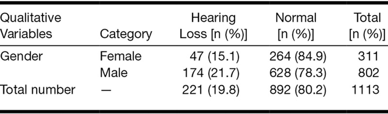
TABLE 2.

Descriptive statistical information of characteristic of workers of each factory in the study cohort

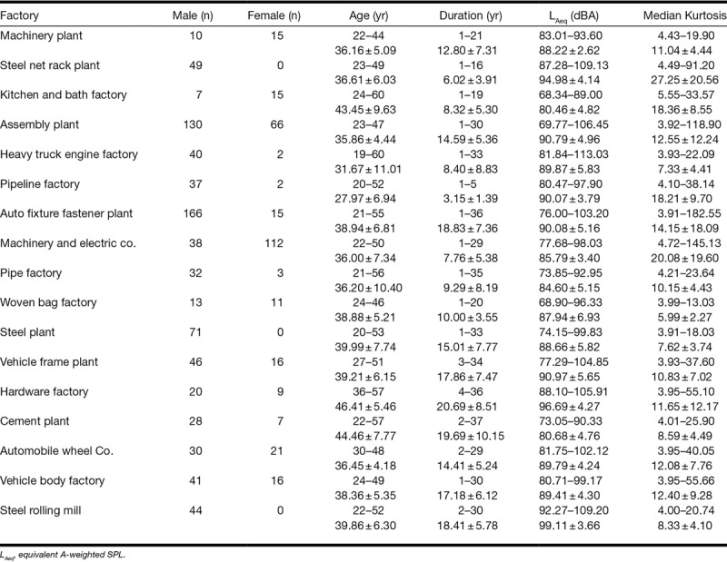
Figure 1 shows scatter plots of the relation between the quantitative independent variables and the average hearing thresholds of the better ear at 1 to 4 kHz for the workers included in the study. It can be seen from Figure 1A, C that the age and equivalent A-weighted SPL (L_Aeq) of the noise approximately obeyed normal distributions. Most workers were between 30 and 50 years old, and the exposure duration was between 1 and 20 years. The values of mean and median kurtosis were scattered in Figure 1D, E. It was noticed that the median kurtosis values were less than 25 and the mean kurtosis values were less than 50 for most workers. The average HTLs of the better ear at 1 to 4 kHz for most workers were between 10 and 30 dB HL. It can be seen from Figure 1C that most of the subjects were exposed to complex noise with the L_Aeq >85 dBA, which exceeded the recommended exposure limit by NIOSH, that is, 85 dB, A-weighting, as 8-hr time-weighted average (NIOSH 1998).

Fig. 1.

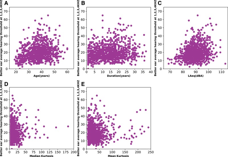
Scatter plots of the relation between the various quantitative variables and the average of hearing threshold levels of the better ear at 1 to 4 kHz (HTL_1–4kHz) for all workers in the study cohort. A, Scatter plot of age vs. HTL_1–4kHz. B, Scatter plot of exposure duration vs. HTL_1–4kHz. C, Scatter plot of equivalent A-weighted SPL (L_Aeq) vs. HTL_1–4kHz. D, Scatter plot of median kurtosis vs. HTL_1–4kHz. E, Scatter plot of median kurtosis vs. HTL_1–4kHz.

Model Construction

Four potential machine learning algorithms were investigated in this study to build classification models for predicting hearing impairment and to build regression models for predicting NIHL quantitatively. Only the architecture of four machine learning classifiers is presented in this paper. The details of their classification and regression algorithms can be found in the references listed below. To train and validate the algorithms, 10 experimental runs were conducted through 10-fold cross-validation.

1. RF model: The RF classifier uses the bootstrap resampling technique to generate N new training sample sets. The new sample sets then are used to train N decision trees. The results of classification depend on the score formed by N decision trees voting. In general, an RF classifier consists of two modules: a training module and a classification module. The overall architecture is shown in Figure 2 (Breiman 2001).

2. Adaboost model: The Adaboost classifier is a highly accurate classifier that takes the single-layer decision tree as the base classification algorithm, training a number of weak learners based on the weight update for the same training set and finally combining these weak learners through weighted fusion to obtain the final strong classifier. The Adaboost classifier architecture is shown in Figure 3 (Freund & Schapire 1997; Nasrabadi 2007; Witten et al. 2016).

3. MLP model: The MLP classifier is a feed-forward neural network. It utilizes a supervised learning technique called backpropagation for training. The algorithm has the advantage of being able to approximate any nonlinear function. In general, an MLP model consists of an input layer, at least one hidden layer, and an output layer. A schematic diagram of the MLP classifier is shown in Figure 4 (Basheer & Hajmeer 2000).

4. SVM model: The SVM classifier is based on establishing a separating hyperplane having maximum distance from the closest points of the training set. This has the advantage of having a strong ability to generalize and can perform very well in solving nonlinear and high-dimensional pattern recognition problems. The principle of an SVM classifier for linearly separable data is shown in Figure 5. For nonlinear problems, it is necessary to choose an appropriate kernel function. A polynomial function was used in this study (Burges 1998; Pontil & Verri 1998; Nasrabadi 2007).

Fig. 2.

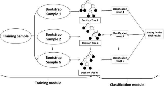
Schematic diagram of the random forest (RF) classifier consisting of a training module and a classification module.

Fig. 3.

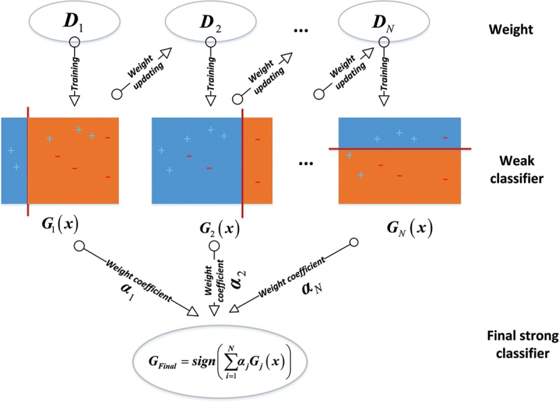
Schematic diagram of the adaptive boosting (Adaboost) classifier. Plus and minus signs represent two classes, respectively.

Fig. 4.

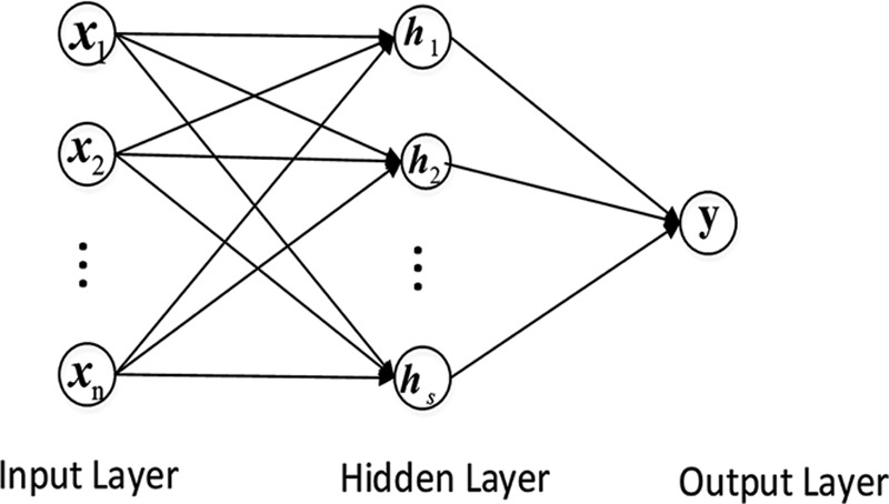
Schematic diagram of the multilayer perceptron (MLP) classification model. Here, represents sample input, represents hidden layer, and represents output layer. The transfer function of the hidden layer vector is 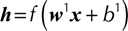, and the output layer neurons is 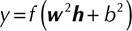, where is the weight matrix between and , is the bias vector of , is the weight matrix between and , and denotes the bias vector of . The activation function is .

Fig. 5.

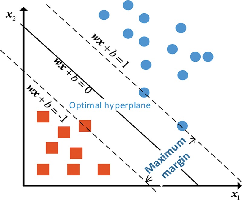
A linear hyperplane learned by training support vector machine (SVM) in two dimensions (D = 2). Squares and circles represent class −1 and class 1, respectively. represents separating hyperplane, and represent margin boundaries, where and are the unknown weights and bias, represents sample input.

Risk Factor Identification

The most predictive features for hearing impairment were identified by feature selection. The selected data values were normalized by min-max normalization technique, and then the p value of each variable was calculated using a t test. Finally, the features for building the SVM, Adaboost, and MLP models were selected based on a significance level of p <0.01. The RF algorithm can handle high-dimensional data and does not require features to be preselected by a t test.

Indices for Model Evaluation

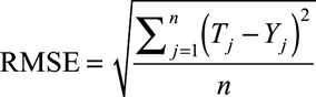
In this study, the indices of (1) the area under the receiver operating characteristic (ROC) curve (AUC) and (2) prediction accuracy were used to measure the performance of the classifiers. A root mean square error (RMSE) was used to evaluate the performance of the regression models. The RMSE is defined as follows:

(1)

where and are the measured and the predicted values of data j, respectively, and n represents the number of measurements. The RMSE indicates the prediction accuracy of regression model. The lower the value of RMSE, the better predictive ability of the regression model.

RESULTS

Risk Factor Identification

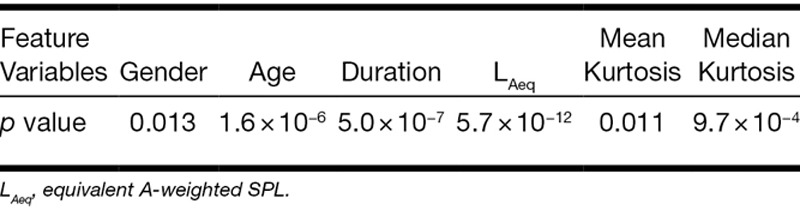
It can be seen from Figure 1 that some of the risk factors appear to be related to hearing loss. Analysis of normalized values by t test revealed that age, exposure duration, L_Aeq, and median kurtosis were significantly associated with hearing loss (p < 0.01) (Table 3). These variables were used for building the three of the prediction models; as noted above the RF model does not require preselection of variables.

TABLE 3.

p values in the study cohort that reflect the relationship between the constructed feature variables and hearing impairment

Performance Evaluation of Different Hearing Impairment Prediction Models

In this study, 10-fold cross-validation was used to conduct the modeling and evaluation for both classification and regression analysis of hearing impairment. Each model was built by calling the Scikit-learn library (Pedregosa et al. 2011) which is one of the well-developed machine learning libraries based on NumPy, SciPy, and Matplotlib. The models were optimized using the grid search method by fine-tuning the parameters of models in the grid (Woodford & Phillips 1997).

The performance of Classification Models

The average ROC curve and the average AUC value of the cross-validation for all models are shown in Figure 6A. It can be reasonably assumed that the models did not over fit the data because the ROC curve corresponding to each model was smooth. However, the ROC curves could not directly reveal which classifier is the best one. Instead, the classifier corresponding to the largest AUC can be considered to have the best function. Thus, the AUC value was used to evaluate the performance of each model in this study. As shown in Figure 6B, the SVM model had the best performance compared with the other models, with an AUC value of 0.808.

Fig. 6.

Hearing impairment predictive performance of four machine learning classification models. Training and testing of all models were conducted with 10-fold cross-validation. A, The mean receiver operating characteristic (ROC) curves of 10-fold cross-validation for four machine learning classification models. B, The average area under the curve (AUC) value of 10-fold cross-validation for four machine learning classification models. Wilcoxon signed-rank test was used to compute p values for AUC of two classifiers using 10-fold cross-validation. The error bars represent the standard deviations of the 10-fold cross-validation. *p < 0.01, **p < 0.001.

In addition, the performance of the machine learning classifier could also be evaluated by the prediction accuracy. The classification accuracies of four models are shown in Figure 7. It can be seen from Figure 7 that SVM had a slightly higher prediction accuracy than the other three models, though the predictive abilities of four models were not significantly different.

Fig. 7.

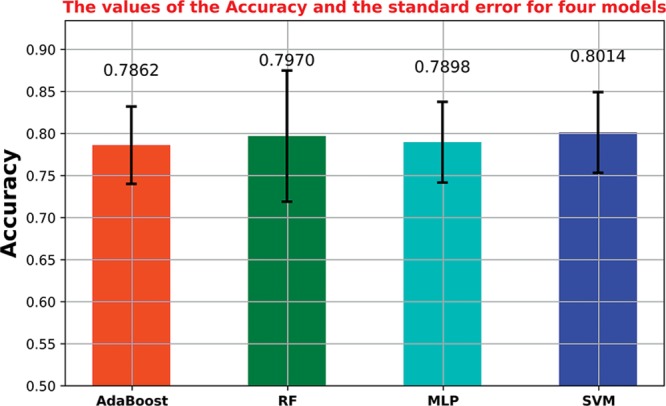
Classification accuracy of various machine learning prediction models. Adaboost, adaptive boosting; MLP, multilayer perceptron; RF, random forest; SVM, support vector machine.

In real applications of machine learning and data mining, the AUC is usually used as the single value for evaluating the predictive performance of a model. The study of Huang and Ling indicated that the AUC is a better measure than accuracy and should replace accuracy when comparing the performance of machine learning algorithms (Huang & Ling 2005). In the present study, both AUC and accuracy indexes showed that the SVM model was the best hearing impairment prediction model.

The Performance of Regression Models

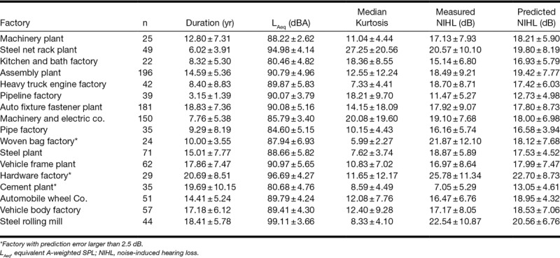
NIHL can be quantitatively predicted by using the regression models with machine learning algorithms. In this study, Adaboost, RF, MLP, and SVM regression models were built to predict NIHL using the features of L_Aeq, exposure duration, and median kurtosis. Measured HTL at each frequency was adjusted by subtracting the median age- and gender-specific HTL from Annex A (ISO-1999 2013), and then the mean age- and gender-adjusted HTLs at 1, 2, 3, and 4 kHz were calculated and used as the definition of NIHL. The RMSE was used to quantify the prediction performances of the regression models. The prediction performances of the four regression models are shown in Table 4. The MLP regression model had the best performance because its RMSE value was the lowest. Therefore, the MLP model was chosen to demonstrate the prediction ability of the developed machine learning regression models. The results are shown in Table 5. Because all audiometric data in this study were collected with a step size of 5 dB using the ascending technique, it is reasonable to assume that the prediction was correct if the difference between predicted and measured NIHL values was less than or equal to 2.5 dB. Comparing the mean predicted NIHL with the measured NIHL from 17 factories in Table 5, it can be seen in Table 5 that the MLP regression model could predict NIHL in all but three factories, that is, the woven bag factory, the hardware factory, and the cement factory.

TABLE 4.

RMSE of four regression models with 10-fold cross-validation

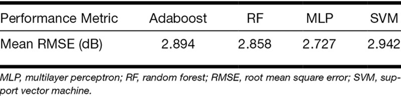
TABLE 5.

Average predicted NIHL of each factory using multilayer perceptron regression model

DISCUSSION

Although machine learning algorithms have been widely applied, little work has been done to predict NIHL from workers exposed to diverse complex industrial noises using these algorithms. Aliabadi et al. (2015) and Farhadian et al. (2015) reported their work of developing NIHL prediction models using neural network algorithms. Using a database with 210 subjects from a steel factory, their results showed that the performance of prediction models was satisfactory. However, it may not be suitable to show the feasibility of the prediction models with such a small size of sample. In this study, four hearing prediction models based on machine learning algorithms, using a noise database with 1,113 subjects from 17 factories, were investigated.

A univariate feature selection method, the t test method, was used in the present study. The p value can be used to rank the input variables according to the degree of correlation with the output variable. It can be seen in Table 3 that the p values of L_Aeq and duration were the smallest. It is not surprising that the equivalent A-weighted SPL and exposure duration are the most important risk factors for noise-induced hearing impairment. Because the definition of hearing impairment by NIOSH is not age and gender adjusted, age and gender were also considered as the risk factors. The kurtosis was used in this study to quantify the impulsiveness of the noise exposure. Because kurtosis was calculated over consecutive 40-s time windows of each shift-long noise record, there were 720 kurtosis values for an 8-hr noise record. The two metrics, mean and median kurtosis, were selected as candidates for risk factors. It can be seen in Table 3 that the importance of all the feature variables was ranked as follows: L_Aeq, duration, age, median kurtosis, gender, and mean kurtosis. Based on a significance level selected (p < 0.01), four risk factors, that is, L_Aeq, duration, age, and median kurtosis, were used in building the noise-induced hearing impairment prediction models.

Despite the large variation of worker’s ages, noise levels, and exposure durations as shown in Figure 1, a prediction accuracy between 78.6 and 80.1% indicated that the four classifiers could be useful tools to assess hearing impairment of workers exposed to various complex occupational noises. A comprehensive evaluation using both the AUC and prediction accuracy showed that the SVM model achieved the best score in classification and thus should be selected as the best tool for predicting hearing impairment from occupational noise exposures in this study.

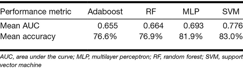
Although this work was based on the NIOSH hearing impairment definition at 1 to 4 kHz, the approaches mentioned above are universal and could be used to predict hearing impairment under different definitions. For example, applying the models to predict hearing impairment based on the Occupational Safety and Health Administration definition, that is, the average HTL of both ears exceeding 25 dB at 1, 2, and 3 kHz, prediction accuracies between 76.6 and 83% were achieved as shown in Table 6. The results in Table 6 verified that the SVM classification model produced the best performance with the highest prediction accuracy of 83%.

TABLE 6.

Performance of four machine learning classification models based on Occupational Safety and Health Administration definition using 10-fold cross-validation.

The results displayed in Table 5 indicated that the MLP regression model could correctly predict the mean NIHL except in three factories marked with an asterisk. Evaluating the noise data from these three failed factories, the sample sizes of these factories were small, indicating that the regression model might not be well trained with small size samples. Among these three failed factories, the cement factory showed the largest prediction error (6 dB). It was noticed that the workers of the cement factory were working in open fields, while the workers of other factories worked in closed workshops. Unlike the subjects working at a fixed position in a closed workshop, the working position for most workers in the cement factory was mobile. Thus, one noise recording for these workers may not be suitable to approximate the noise exposure over the lifetime of work.

In this pilot study, four machine learning algorithms were used to build both classification and regression models for noise-induced hearing impairment prediction. Although the SVM and MLP algorithms demonstrated their appropriateness for classification and regression analyses, Adaboost and RF algorithms also performed well in solving classification and regression problems. As shown in Figure 7, Adaboost and RF could achieve a similar classification accuracy as SVM and MLP. In the regression study, the Adaboost and RF even scored smaller RMSE than SVM. Thus, Adaboost and RF may also have potential value in predicting hearing impairment.

Though the classification and regression models using the four machine learning algorithms performed well in predicting hearing impairment, the performance could be further improved by acquiring more data from a larger number of subjects with well-documented and diverse exposures. In addition to the feature variables used in the above prediction models, more information relating to hearing loss, such as the octave band noise level, kurtosis in frequency domain, smoking history, blood pressure, and genes related to susceptibility of hearing loss, should be collected. Another possible method to enhance performance would be to develop a prediction model for exposure groups that share very similar noise characteristics, thus producing a more homogeneous group of cohorts. With more noise data being collected and more relevant risk factors being considered, NIHL evaluation using machine learning can be very useful to hearing conservation practices.

CONCLUSIONS

This pilot study demonstrated that machine learning algorithms are potential tools for the prediction of noise-induced hearing impairment in workers exposed to diverse complex industrial noises.

ACKNOWLEDGMENTS

Y. Z., J. L., Y. T., and W. Q. designed and performed project; M. Z. and H. X. conducted field investigation, data collection, and quality control; Y. Z. and Y. L. analyzed the data; Y. Z. wrote the paper; and J. L., Y. T., and W. Q. provided critical revision and discussion. All authors discussed the results and implications and commented on the manuscript at all stages. We thank all reviewers and editors who helped to improve this work.

This work was partially supported by Grant 200-2015-M-63857, 200-2016-M-91922 from the National Institute for Occupational Safety and Health, USA; Grant N00014-17-1-2198 from Office of Naval Research, USA; Grant 2015C03039 from Key Research and Development Program of Zhejiang Province, China; and Grant 81771936 from National Natural Science Foundation, China.

REFERENCES

- Aliabadi M., Farhadian M., Darvishi E. Prediction of hearing loss among the noise-exposed workers in a steel factory using artificial intelligence approach. Int Arch Occup Environ Health, 2015). 88, 779–787. [DOI] [PubMed] [Google Scholar]
- Atherley G. R. Noise-induced hearing loss: The energy principle for recurrent impact noise and noise exposure close to the recommended limits. Ann Occup Hyg, 1973). 16, 183–194. [DOI] [PubMed] [Google Scholar]
- Barker D. H., Quittner A. L., Fink N. E, et al. ; CDaCI Investigative Team. (Predicting behavior problems in deaf and hearing children: The influences of language, attention, and parent-child communication. Dev Psychopathol, 2009). 21, 373–392. [DOI] [PMC free article] [PubMed] [Google Scholar]
- Basheer I. A., Hajmeer M. Artificial neural networks: Fundamentals, computing, design, and application. J Microbiol Methods, 2000). 43, 3–31. [DOI] [PubMed] [Google Scholar]
- Breiman L. Random forests. Mach Learn, 2001). 45(1), 5–32. [Google Scholar]
- Burges C. J. C. A tutorial on Support Vector Machines for pattern recognition. Data Min Knowl Disc, 1998). 2(2), 121–167. [Google Scholar]
- Chan J. C. W., Paelinckx D. Evaluation of Random Forest and Adaboost tree-based ensemble classification and spectral band selection for ecotope mapping using airborne hyperspectral imagery. Remote Sens Environ, 2008). 112(6), 2999–3011. [Google Scholar]
- Cherkassky V., Mulier F. M. Learning From Data: Concepts, Theory, and Methods. 2007). New York, NY: John Wiley & Sons. [Google Scholar]
- Davis R. I., Qiu W., Hamernik R. P. Role of the kurtosis statistic in evaluating complex noise exposures for the protection of hearing. Ear Hear, 2009). 30, 628–634. [DOI] [PubMed] [Google Scholar]
- Drucker H., Wu D., Vapnik V. N. Support vector machines for spam categorization. IEEE Trans Neural Netw, 1999). 10, 1048–1054. [DOI] [PubMed] [Google Scholar]
- Farhadian M., Aliabadi M., Darvishi E. Empirical estimation of the grades of hearing impairment among industrial workers based on new artificial neural networks and classical regression methods. Indian J Occup Environ Med, 2015). 19, 84–89. [DOI] [PMC free article] [PubMed] [Google Scholar]
- Freund Y., Schapire R. E. A decision-theoretic generalization of on-line learning and an application to boosting. J Comput Syst Sci, 1997). 55(1), 119–139. [Google Scholar]
- Graves A., Mohamed A. R., Hinton G. Speech recognition with deep recurrent neural networks. Proc. IEEE Int Conf Acoust Speech Signal Process, 2013). 1, 6645–6649. [Google Scholar]
- Guberan E., Fernandez J., Cardinet J, et al. Hazardous exposure to industrial impact noise: Persistent effect on hearing. Ann Occup Hyg, 1971). 14, 345–350. [DOI] [PubMed] [Google Scholar]
- Hamernik R. P., Qiu W. Energy-independent factors influencing noise-induced hearing loss in the chinchilla model. J Acoust Soc Am, 2001). 110, 3163–3168. [DOI] [PubMed] [Google Scholar]
- Hamernik R. P., Qiu W., Davis B. The effects of the amplitude distribution of equal energy exposures on noise-induced hearing loss: The kurtosis metric. J Acoust Soc Am, 2003). 114, 386–395. [DOI] [PubMed] [Google Scholar]
- Henderson D., Subramaniam M., Boettcher F. A. Individual susceptibility to noise-induced hearing loss: An old topic revisited. Ear Hear, 1993). 14, 152–168. [DOI] [PubMed] [Google Scholar]
- Huang J., Ling C. X. Using AUC and accuracy in evaluating learning algorithms. Ieee T Knowl Data En, 2005). 17(3), 299–310. [Google Scholar]
- ISO-1999. (Estimation of noise-induced hearing loss. 2013). Geneva, Switzerland: International Organization for Standardization. [Google Scholar]
- Konings A., Van Laer L., Van Camp G. Genetic studies on noise-induced hearing loss: A review. Ear Hear, 2009). 30, 151–159. [DOI] [PubMed] [Google Scholar]
- Lie A., Skogstad M., Johannessen H. A, et al. Occupational noise exposure and hearing: A systematic review. Int Arch Occup Environ Health, 2016). 89, 351–372. [DOI] [PMC free article] [PubMed] [Google Scholar]
- Mian A. S., Bennamoun M., Owens R. An efficient multimodal 2D-3D hybrid approach to automatic face recognition. Ieee T Pattern Anal, 2007). 29(11), 1927–1943. [DOI] [PubMed] [Google Scholar]
- Mizoue T., Miyamoto T., Shimizu T. Combined effect of smoking and occupational exposure to noise on hearing loss in steel factory workers. Occup Environ Med, 2003). 60, 56–59. [DOI] [PMC free article] [PubMed] [Google Scholar]
- Nasrabadi N. M. Pattern recognition and machine learning. J Electron Imaging, 2007). 16(4), 049901. [Google Scholar]
- NIOSH. (NIOSH – Criteria for a Recommended Standard: Occupational Noise Exposure. 1998). Cincinnati, Ohio: National Institute for Occupational Safety and Health. [Google Scholar]
- Nomura K., Nakao M., Yano E. Hearing loss associated with smoking and occupational noise exposure in a Japanese metal working company. Int Arch Occup Environ Health, 2005). 78, 178–184. [DOI] [PubMed] [Google Scholar]
- Pedregosa F., Varoquaux G., Gramfort A, et al. Scikit-learn: Machine Learning in Python. J Mach Learn Res, 2011). 12, 2825–2830. [Google Scholar]
- Pelegrin A. C., Canuet L., Rodríguez Á. A, et al. Predictive factors of occupational noise-induced hearing loss in Spanish workers: A prospective study. Noise Health, 2015). 17, 343–349. [DOI] [PMC free article] [PubMed] [Google Scholar]
- Pontil M., Verri A. Properties of support vector machines. Neural Comput, 1998). 10, 955–974. [DOI] [PubMed] [Google Scholar]
- Qiu W., Davis B., Hamernik R. P. Hearing loss from interrupted, intermittent, and time varying Gaussian noise exposures: the applicability of the equal energy hypothesis. J Acoust Soc Am, 2007). 121, 1613–1620. [DOI] [PubMed] [Google Scholar]
- Qiu W., Hamernik R. P., Davis B. The kurtosis metric as an adjunct to energy in the prediction of trauma from continuous, nonGaussian noise exposures. J Acoust Soc Am, 2006). 120, 3901–3906. [DOI] [PubMed] [Google Scholar]
- Qiu W., Hamernik R. P., Davis R. I. The value of a kurtosis metric in estimating the hazard to hearing of complex industrial noise exposures. J Acoust Soc Am, 2013). 133, 2856–2866. [DOI] [PMC free article] [PubMed] [Google Scholar]
- Settouti N., Bechar M. E., Chikh M. A. Statistical comparisons of the top 10 algorithms in data mining for classification task. Int J Interact Multi, 2016). 4(1), 46–51. [Google Scholar]
- Witten I. H., Frank E., Hall M. A, et al. Data Mining: Practical Machine Learning Tools and Techniques. 2016). San Francisco, CA: Morgan Kaufmann. [Google Scholar]
- Woodford C., Phillips C. Numerical Methods With Worked Examples. 1997). London, United Kingdom: Chapman and Hall. [Google Scholar]
- Xie H. W., Qiu W., Heyer N. J, et al. The use of the kurtosis-adjusted cumulative noise exposure metric in evaluating the hearing loss risk for complex noise. Ear Hear, 2016). 37, 312–323. [DOI] [PMC free article] [PubMed] [Google Scholar]
- Zhao Y. M., Qiu W., Zeng L, et al. Application of the kurtosis statistic to the evaluation of the risk of hearing loss in workers exposed to high-level complex noise. Ear Hear, 2010). 31, 527–532. [DOI] [PubMed] [Google Scholar]
REFERENCE NOTE
- Syeda M., Zhang Y. Q., Pan Y. Parallel granular neural networks for fast credit card fraud detection. Proc. IEEE Int Conf Fuzzy Systems, 2002). 1(2), 572–577. [Google Scholar]