Controlling fluid-induced seismicity during a 6.1-km-deep geothermal stimulation in Finland

Near–real-time seismic monitoring and injection control limits induced earthquakes in urban geothermal reservoir stimulation.

Abstract

We show that near–real-time seismic monitoring of fluid injection allowed control of induced earthquakes during the stimulation of a 6.1-km-deep geothermal well near Helsinki, Finland. A total of 18,160 m³ of fresh water was pumped into crystalline rocks over 49 days in June to July 2018. Seismic monitoring was performed with a 24-station borehole seismometer network. Using near–real-time information on induced-earthquake rates, locations, magnitudes, and evolution of seismic and hydraulic energy, pumping was either stopped or varied—in the latter case, between well-head pressures of 60 and 90 MPa and flow rates of 400 and 800 liters/min. This procedure avoided the nucleation of a project-stopping magnitude M_W 2.0 induced earthquake, a limit set by local authorities. Our results suggest a possible physics-based approach to controlling stimulation-induced seismicity in geothermal projects.

INTRODUCTION

Enhanced geothermal systems (EGSs) hold the promise of using the ubiquitous heat energy of Earth. However, EGS typically requires opening—“stimulation”—of fluid flow channels, the by-products of which are earthquakes (1). Triggered and induced seismicity have terminated important geothermal project in Switzerland (2, 3). In addition, a link between the occurrence of a M_W (moment magnitude) 5.5 earthquake that occurred in Pohang, South Korea, and the development of nearby EGS has been hypothesized (4, 5). The result has been the questioning and compromising of the commercial viability of EGS despite its baseload and environmental advantages. Finding safe stimulation strategies is thus critical for reducing the negative socioeconomic impact of EGS-related induced seismicity.

Previous efforts aiming at controlling seismicity during fluid injection projects date back to the 1960s in early deep injection tests such as the Rocky Mountain Arsenal (6) and Rangely oil field, Colorado (7). For the latter, the frictional properties of reservoir rocks and in situ stress measurements were used to define a critical fluid pressure beyond which earthquakes were induced. On the basis of a model relating fluid pressure and resulting seismicity, an attempt was made to control seismic activity by adjusting the injection schedule and to keep the fluid formation pressure below a critical level, at which the rate of induced earthquakes was observed to increase. More recently, several studies focused on limiting the maximum magnitude of seismic events. Event magnitudes have been related to different parameters including, e.g., total injected fluid volume (8, 9), elastic energy stored in the rock mass (10), or the size of pore pressure perturbed zone (11). However, successful efforts to maintain event magnitudes during stimulation below a critical threshold level have not yet been reported.

Here, we show that high-precision, near–real-time monitoring and analysis of seismic data feeding a traffic light system (TLS) allowed safe stimulation of the world’s deepest EGS project so far (Fig. 1). This St1 Deep Heat Oy energy-company joint pilot project is located in the Helsinki metropolitan area, on the urban campus of Aalto University (fig. S1). The aim is to produce a sustainable baseload for the campus area’s district heating network, with development costs being offset by saving in imported fuel and reduced CO₂ emissions.

Fig. 1. Schematic view of the project site (see fig. S1 for a map view).

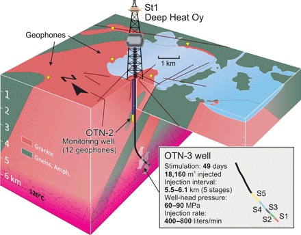
The location of stimulation stages S1 to S5 into the bottom open hole section and basic stimulation parameters are shown in the inset.

A 6.4-km measured depth (MD) stimulation well, OTN-3, and a 3.3-km observation well, OTN-2, were drilled mostly not only with down-the-hole air and water hammer methods but also with rotary methods for steering purposes. Both wells are entirely located in crystalline Precambrian Svecofennian basement rocks consisting of granites, pegmatites, gneisses, and amphibolites. The last 1000 m of OTN-3 was drilled inclined at 42° to the northeast (NE), left uncased, and completed with a five-stage stimulation assembly. OTN-2 was drilled vertically, 10 m offset from OTN-3 (fig. S1, inset).

In June and July 2018, a total of 18,160 m³ of water was pumped into the rock formation at true vertical depths of 5.7 to 6.1 km over a period of 49 days. This included moving injection intervals and stoppages of a few days at various points during the stimulation. The stimulation was injection rate–controlled, with flow rates varying at discrete levels between 400 and 800 liters/min (typically just above the technical lower limit of 400 liters/s). This resulted in measured well-head pressures ranging from 60 to 90 MPa and below an upper safety limit for the pumps at 95 MPa. Induced seismicity was monitored by a three-tier seismic network, all telemetered to the project site. The key element was a 12-level vertical array of three-component seismometers placed at depths of 2.20 to 2.65 km in the OTN-2 well (fig. S1). This array was complemented by an additional 12-station satellite network with seismometers installed in 0.3- to 1.15-km-deep wells at 0.6- to 8.2-km lateral offsets. In addition, a 14-station strong-motion sensor network was placed at nearby critical infrastructure sites.

The objective of the borehole array and satellite network was to provide accurate induced-earthquake hypocenter locations and magnitudes for both industrial (stimulation of a permeable fracture network) and regulatory (TLS) purposes. The strong-motion network was aimed at providing direct evidence of potentially damaging shaking. Background seismicity in the campus region is very sparse. The closest event with claims of building damage in recent years was a M_W 2.4 event in 2011, located 50 km to the NE from the project site. Two detected microearthquakes were reported to have occurred within 2 km of the drill site in 2011. These were M_W 1.7 and 1.4 events and were placed at a depth of 1 km by the Helsinki area network (fig. S1). Both borehole array and satellite network were operating intermittently since 2016, detecting no locatable microseismicity at depth close to the inclined deeper section of the OTN-3 well.

A M_W 2.0 event (see Materials and Methods for details of derivation of the TLS system) was prescribed by local authorities as the upper limit to the earthquake that could be induced at the depth of the stimulation. This limit was based on the expected peak ground velocity (PGV) at the surface from such an earthquake—a limit substantially below local building codes. Exceeding M_W 2.0 (red TLS conditions) would trigger the shut-in of the well, and no further injection was allowed without new approvals from Finnish authorities. This challenging prescribed limit accounted for potential nuisance effects to the local population and existence of sensitive instrumentation and supercomputing facilities near the St1 project site. Larger events with M_W ≥ 1.3 (amber TLS conditions) needed to be reported to local authorities within 20 min, but they were allowed without further consultation.

RESULTS

Earthquakes located within an epicentral distance of 5 km and at depths of 0.5 to 10 km of the OTN-3 well-head were considered for the TLS. During the stimulation, a total of 8412 events meeting these criteria were reported to the TLS operator within a maximum delay of 5 min (15 min with manual refinement of events) and included magnitude and hypocenter estimate. Out of these, 6150 earthquakes formed the initial catalog for evaluating the industrial success of the stimulation. The latter events had larger signal-to-noise ratios and were deemed best for determining their locations and magnitudes.

Together with a TLS decision tree prescribing the course of action after the exceedance of M_W 1.3, the near–real-time earthquake information was used by the TLS operator to provide feedback to the stimulation engineers, who controlled pumping rates and well-head pressures. The original stimulation strategy was also modified, in response to the occurrence of enhanced seismic activity and after the improved understanding of the reservoir seismic response. This ultimately allowed us to keep the maximum magnitude below the M_W 2.0 limit. By the completion of the stimulation, the maximum induced event was M_W 1.9. Since then, the activity ceased to a few detectable events per hour, and until the end of monitoring (2 October 2018), no event larger than M_W 1.3 occurred in the vicinity of the OTN-3 well.

Figure 2A shows temporal changes in hydraulic and seismic parameters during the 49 days of injection and 9 days following shut-in of the well. Pumping was performed in five injection phases (P1 to P5 in Fig. 2A), each lasting 2 to 14 days. These phases were intended to be pumped through corresponding stimulation stages S1 to S5 located along the open hole section of the OTN-3 well (Fig. 1, inset). However, the phase P2 stimulation was likely performed through the stage S3 port due to malfunctioning of the S2 port (for details, see Materials and Methods). Each phase consisted of multiple subphases of continuous injection performed typically at a constant injection rate, alternating with resting periods, when injection was stopped. The cumulative injected fluid volume per subphase is presented as the blue line in Fig. 2A.

Fig. 2. Evolution of seismic source and statistical properties of induced seismicity in response to fluid injection.

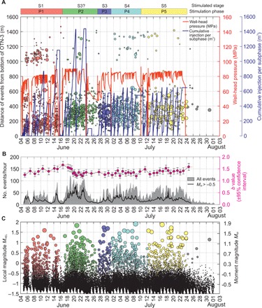
Temporal evolution of double-difference relocated seismicity (n = 1977) plotted as the distance from the bottom of OTN-3 and color-encoded by stimulation phase (A). Well-head pressure and cumulative injection per stimulation subphase are shown as solid red and dark blue lines, respectively. (B) Gutenberg-Richter (GR) b-value changes (magenta dots). The evolution of seismic event rate calculated for all events above magnitude of completeness and for a catalog with M_W > −0.5 is shown in gray and superposed black line, respectively. (C) Moment (M_W) and local Helsinki magnitudes (M_LHEL) of seismic events. Events detected but not located are shown as black points (note day-night detection level variations).

Figure 3 presents hypocenter map (Fig. 3A) and southwest (SW)–NE depth section (Fig. 3B) of 1977 earthquakes relocated from the initial catalog of 6150 using the double-difference method (12). Earthquake hypocenters are shown as circles color-coded with injection phase and with size proportional to the respective moment magnitude. The first recorded earthquake was located at the bottom of the open hole section of the injection well, approximately 3 hours after injection operations started on 4 June, and at a well-head pressure of 7 MPa. For the stress magnitudes based on extrapolated borehole breakout measurements and a friction coefficient of 0.6, favorably oriented faults were expected to be close to failure (13), with the consequent onset of seismic events at a moderate fluid pressure increase (see Materials and Methods). Seismic activity increased substantially in the following 6 hours of injection, starting once the well-head pressure exceeded 70 MPa. No notable time delays between injection pressure, flow rate changes, and the occurrence of seismicity were found during the entire stimulation (Fig. 2). There was also no evidence of Kaiser effect (14), where activity at a certain spot would start only after previous pressure levels were exceeded.

Fig. 3. Induced seismicity hypocenters during stimulation campaign.

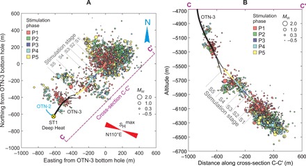
(A) Map view and (B) SW-NE depth section showing double-difference relocated seismicity (n = 1977) color-coded with stimulation phase. Injection stages S1 to S5 are colored accordingly from the bottom of the open hole (6.4 km MD) toward the casing shoe (5.4 km MD) of OTN-3. The size of each event is proportional to the moment magnitude.

A relatively quick dissipation of strain energy accumulated from fluid injection is consistent with a sharp decrease in the seismic activity following shut-in phases (Fig. 2). Ultimately, 1 week after the final shut-in of OTN-3 on 23 July, the hourly seismicity rate dropped from a maximum of 120 down to a few detected small events (Fig. 2B). We also noted that the seismic activity and seismic radiated energy release correlated well in both time and magnitude with the product of injection rate and well-head pressure (=hydraulic energy E_H). The seismicity, and thus the seismic moment/seismic radiated energy release, was primarily sensitive to increases in the well-head pressure. Maintaining the well-head pressure and flow rate at 80 MPa and 400 liters/min, respectively, reduced the cumulative P1 seismic moment release to 50% of that observed in phases P2, P4, and P5. This is presented in Fig. 4A, which shows temporal changes in cumulative seismic moment for each injection phase. Similar low levels of seismic moment release as in P1 did not occur in the subsequent phases. Instead, phase P2 well-head pressures exceeding 90 MPa combined with longer and continuous periods of pumping (Fig. 2A) accelerated the seismic moment/energy release rate (Fig. 4, A and B). This was manifested in a series of larger events (up to M_W = 1.8; Fig. 2C) that forced an end to P2.

Fig. 4. Evolution of seismic moment, radiated energy and hydraulic energy release during stimulation.

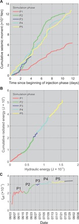
(A) Cumulative seismic moment release with time. (B) Cumulative radiated seismic energy release as a function of hydraulic energy. (C) Seismic injection efficiency I_E changes with time.

OTN-3–induced seismicity showed a monotonic increase of maximum earthquake magnitude with the cumulative injected fluid volume (Fig. 5). This increase followed the trend predicted by the recently introduced fracture mechanics–based model of Galis et al. (10). It was also close to that presented by van der Elst et al. (15), but remaining much lower than the upper limit predicted by McGarr’s (8) model. According to Galis et al., this behavior suggests that the maximum magnitude depends on both the regional tectonic stress and the imposed local fluid pressure controlling the total elastic energy stored in the system. Considering the observed trend in maximum magnitude evolution with the injected fluid volume, it was expected that the M_W 2.0 red alert threshold would likely be exceeded once the targeted fluid volume of 20,000 m³ was injected (note that the dashed line in Fig. 5 parameterized by γ = 2 × 10⁶ presents a post-stimulation assessment of the maximum magnitude evolution, with fluid volume accounting for actual reservoir and seismicity parameters). Therefore, following Galis et al.’s model, our pumping strategy was modified after phase P2. Well-head pressures were limited to about 86 MPa (see more detailed timeline in Materials and Methods). This pressure level was established by a trial-and-error procedure in an attempt to limit accumulation of stored elastic energy due to injection and reach the targeted cumulative injection volume. In a further adjustment to also reduce stored elastic strain energy by fluid pressure dissipation, the injection subphases of P4 and P5 were reduced in duration to 18 hours with 6-hour rest periods (see Fig. 2). As a final measure, pumping was immediately stopped and resting periods extended whenever a large seismic event with M_W > 1.7 occurred (Fig. 2).

Fig. 5. Temporal evolution of maximum observed seismic moment versus cumulative volume of injected fluid at each phase (P1 to P5).

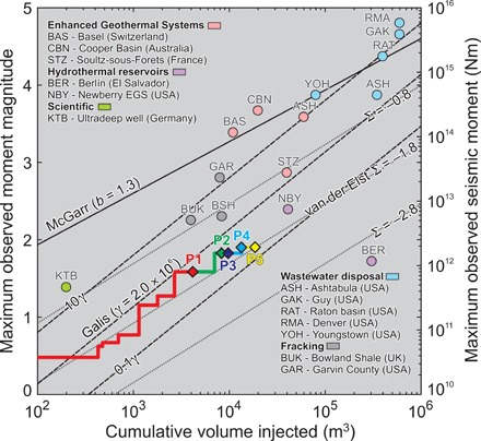
Colored circles are from various injection projects (8, 19, 20). Maximum magnitude estimates using different models are shown with solid, dashed, and dotted lines (8, 10, 15). The γ and b parameter values used in (8, 10) were calculated after the stimulation, assuming geomechanical and seismic parameters from this study, and plotted for comparison with the observed evolution of seismic moment (see Materials and Methods).

These changes in the injection strategy after P2 were kept until the end of the stimulation. They seemingly stabilized seismic energy release with respect to hydraulic energy in phases P3 to P5, although still at a slightly higher release rate of radiated energy compared to P1 (Fig. 4B). Equivalently, the seismic injection efficiency I_E, the ratio of cumulative radiated energy to hydraulic energy E_H (16), stabilized after P2 at a higher level (Fig. 4C). The flattening of I_E suggested that some balance between strain energy buildup and dissipation had been achieved, with I_E only slightly increasing during the final injection phases. We believe that this approach allowed a successful completion of the stimulation plan while avoiding a project derailing M_W > 2.0 red alert induced earthquake.

Upon completion of injection, the seismic data were reprocessed to further reduce the magnitude detection threshold and to refine earthquake source parameters. This aimed at improving our understanding of the spatial and temporal development of induced seismicity, and investigates factors leading to observed behavior of maximum magnitude. This reprocessing (see Materials and Methods) enlarged the original near–real-time industrial seismic catalog to 43,882 events, with magnitudes down to M_W = −0.6. From this extended catalog, all events with M_W > 0.7 were manually reviewed. A further subset of 1977 best-recorded earthquakes that occurred in the immediate vicinity to the injection well (Fig. 3) was relocated using the double-difference relocation method (12). This improved the relative hypocenter precision down to ~27 and ~66 m for 68 and 95%, respectively, of the relocated catalog.

DISCUSSION

The induced seismicity occurred in three main spatially separated clusters located along the injection interval of OTN-3 (Fig. 3). The clusters were active simultaneously but showed no clear spatial or temporal links to the injection ports opened during specific stimulation stages. An additional small fourth cluster located near the upper end of the open hole was developed during the last injection phases (P4 and P5). These and other engineering observations including large caliper logged along the open hole section suggest that the injected fluid might pass along the damaged wall rock of the OTN-3 well, bypassing the stage packers.

The events within each cluster trended and expanded in the southeast (SE)–northwest (NW) direction as stimulation progressed. This direction is subparallel to the direction of maximum horizontal stress (S_H^max) (13) and coincides with surface features mapped in the vicinity of the project site (17). The upper two main clusters roughly correlate with locations where drilling progress was difficult, including a drill string jammed at the beginning of inclined section OTN-3 while the well was drilled, and small fluid losses observed in this area. In addition, anomalies in well logs including temperature fluctuations, caliper logs, and higher density of borehole breakouts were encountered in these intervals, suggesting the existence of discrete, broad damage zones. It is then likely that fluids propagating along the damaged wall rock of the OTN-3 well, beyond the stimulation tool, were entering all damage zones concurrently, regardless of the active injection stage. The spatially largest hypocenter cluster occurred at and below the bottom of OTN-3. It was active throughout the whole stimulation, with seismicity slowly deepening with time toward the NE.

Source sizes calculated for 56 events with M_W > 1.1 using spectral analysis (see Materials and Methods) display source radii of 11 to 34 m, assuming circular source model of Madariaga (18). Combined with estimated hypocenter precision and spatial extent of clusters, this indicates that the hypocenter cloud shows no evidence for alignment along a large fault, but rather appears as the activation of a broad network of distributed fractures. Moreover, a significant drop-off in the number of events above M_W > 1.5 exists in the Gutenberg-Richter (GR) distribution of the induced earthquakes (fig. S4). Hence, the stimulated volume may not contain faults large enough to sustain larger events. Alternatively, the fluid injection did not store enough elastic energy in the reservoir to support a runaway rupture on a large fault (10).

The activation of a distributed fracture network is supported by comparison of empirical data of seismic injection efficiency I_E from various sites. For St1, the observed values of I_E ranges from 2.0 × 10⁻³ in P1 to 3.2 × 10⁻³ in P5 (Fig. 4C). This range of values is higher than the I_E < 10⁻⁵ commonly reported for hydraulic fracturing campaigns, where new fractures are being created (19–21). It is, however, lower than the I_E reported for the EGS stimulations at Basel and Cooper Basin (19), where I_E ranged between 10⁻² and 1. This is expected, as maximum magnitudes at these sites were also larger (Fig. 5): 3.4 at Basel and 3.7 at Cooper Basin (22, 23). At Basel and Cooper Basin, nearby larger faults were apparently activated. Combined, the low I_E values during OTN-3 stimulation, the clustering of event locations in broad zones, and the statistically significant breakdown of GR b value at large magnitudes would suggest that the OTN-3 stimulation activated a preexisting small-scale fracture network rather than a prominent, single, large fault.

The catalog of 43,882 induced earthquakes covering the stimulation period and 1 week after the stimulation indicates that between the GR b value increased in phase P1 from 1.2 to 1.6 (Fig. 2B). This may correspond to the reactivation/creation fracture network at the beginning of injection. However, the b value returned to and then remained at ~1.3 during the subsequent stimulation phases P2 to P5. Thus, the earthquake hazard correlated primarily with the seismic activity—the GR a value (see Fig. 2B)—rather than the ratio of small to large events, the GR b value.

Presumably, tectonic loading rates at the St1 site are lower compared to other sites located close to active faults (e.g., as in the Rhine Graben/Basel and close to the Alps). If the temporal changes in b value are a function of the mean crustal stress evolution as proposed by others (24), then our observations suggest that the OTN-3 stimulation did not lead to a notable and persistent increase in deviatoric stresses during later injection phases. This is different from the observations at the Basel EGS site, where b values have been observed to decrease (25) with progressing injection, likely associated with a long-lasting stress perturbation. In addition, the observed seismicity shows no substantial spatial clustering in rescaled interevent times and distances (fig. S5) (26), indicating minor earthquake interaction/triggering and low stress transfer (27). This suggests that stress changes induced by the OTN-3 stimulation may have been quickly relaxed by the small-scale seismic activity along weak fractured zones.

For critically stressed rock, small pore pressure changes are sufficient to activate favorably oriented faults and fractures, as observed in this and similar stimulation projects. Our observations suggest that fluid injection activated a network of preexisting faults and fractures. In particular, the located seismic activity indicated growth of three-dimensional (3D) ellipsoidal event clusters rather than activation of a prominent fault structure. We observed that maximum induced-earthquake magnitudes scaled with the injected fluid volume closely following a trend predicted by a fracture mechanics–based model (10), which relates maximum magnitudes of self-arrested earthquakes to the injected fluid volume. We adjusted the injection rates in an effort to constrain the amount of stored elastic energy available for rupture propagation, maintaining a low ratio of radiated energy to hydraulic energy input. This was achieved in an iterative procedure by reducing injection rates and extending waiting periods between pumping phases. Adjusting the stimulation schedule to the observed evolution of induced seismicity allowed us to successfully prevent the occurrence of larger events exceeding a TLS-defined red alert. It is possible that the advantageous geological and tectonic reservoir features and favorable stress (transfer) conditions contributed to project success, although their detailed role needs to be further investigated. We expect that different tectonic settings and geological boundary conditions would require specific adjustments of injection schedules.

Controlling injection-induced seismicity is of crucial importance for public acceptance of enhanced geothermal energy projects. The two cases of EGS in Basel (2, 3) and Pohang (4, 5) showed a broad negative socioeconomic impact of EGS-associated seismicity, even regardless of whether, in the latter case of Pohang, the causal relation between EGS operations and the occurrence of large event is a subject of pending investigation. This negatively affects the support of communities to geothermal energy, as well as increases the economic costs of EGS implementation due to the enhanced risk.

In St1 project at the Aalto University campus, we used near–real-time seismic monitoring to modify stimulation parameters to successfully limit induced-earthquake magnitudes to the maximum allowable M_W = 2.0. This result was achieved by close cooperation of seismologists, site operator, TLS teams, and local authorities during the stimulation operation.

MATERIALS AND METHODS

Site description

The St1 drill site is located on crystalline Precambrian Svecofennian basement rocks. These are only locally covered by 20 m or less of quaternary glacial deposits and clay-rich soils. They represent a deep crustal section of deformed metamorphic and intrusive granites, pegmatites, quartzo-feldspathic gneisses, and amphibolites (28). In the course of post-Precambrian tectonics, Late Mesozoic plate motions, and Holocene glacial rebound, the basement rocks became folded, foliated, jointed, and faulted.

On the basis of inversion of regional earthquake focal mechanisms, the current local maximum horizontal stress is oriented N110°E (29). Roughly normal to this and ~8 km to the NW of the drill site is the ~50-km-long, left-lateral Porkkala-Mäntsälä fault zone (30). The largest instrumentally recorded earthquake on this fault was an M2.6 event in 2011 (31). About 1.5 km to the SE is a similarly oriented and long, but apparently inactive, thrust fault, likely dipping to the SE (17). Drill bit seismic data recorded at the site suggest that an additional SE to SW 70° to 80° dipping structure 1 to 2 km to the NW may intersect the injection well at depths of 5.4 to 6.2 km. The closest known earthquakes to the drill site were M_W 1.7 and M_W 1.4 events, recorded in 2013 (31).

Stress magnitudes at the drill site were estimated from wellbore breakouts and minifrac shut-in pressures measured down to a depth of 1.8 km (13). Extrapolated to a depth of 6.1 km, these were estimated to be S_H^min = 110 MPa, S_V = 180 MPa, and S_H^max = 240 MPa. Pore pressures were assumed to be hydrostatic, equaling to approximately 60 MPa. Assuming a friction coefficient of 0.6, these results suggested that optimally oriented fractures and faults could be readily activated with moderate fluid pressure increases.

Seismic network

The real-time telemetered network monitoring the stimulation campaign was composed of 24 borehole seismographs, fabricated, installed, and operated by Advanced Seismic Instrumentation and Research (www.asirseismic.com; fig. S1). The 12-level borehole array of three-component 15-Hz natural frequency Geospace OMNI-2400 geophones was sampled at 2 kHz. This array was placed at depths of 2.20 to 2.65 km in the OTN-2 well. Additional 12-station three-component f_N = 4.5 Hz Sunfull PSH geophones sampled at 500 Hz were installed in 0.30- to 1.15-km-deep wells. These surrounded the project site at 0.6- to 8.2-km epicentral distances. These two networks were operating months before the start of stimulation with no event. Last, a 14-station ground motion network was placed at critical surface sites in the Helsinki area to monitor the ground motions for the purpose of TLS operation. This network was not used in automated near–real-time processing discussed after the following section.

Traffic light system

The TLS consisted of green, amber, and red thresholds, where exceedances of an amber threshold required notifications to be communicated and additional analyses to be performed; exceedances of a red threshold additionally required stimulation activities to be stopped as quickly as safely possible. The selection of thresholds was based on PGV thresholds and their impacts on the population and the built environment. These PGV thresholds were then translated into magnitude thresholds using both global (32) and local (33, 34) ground motion prediction equations (GMPEs). More specifically, magnitudes associated with PGV thresholds were selected on the basis of a conservatively low probability (i.e., either 10 or 2%) that the seismic event would result in a PGV at the surface sufficient to cause a TLS exceedance, based on the GMPE uncertainties. Implemented TLS thresholds were based on either exceeding both a PGV and local “Helsinki” magnitude, M_LHEL (33, 34), or a separate scenario where only a magnitude was exceeded. The former was developed to confirm that monitored surface vibrations were related to seismic events, while the latter was developed in the event that an unacceptable surface expression would occur in an area absent of surface monitoring.

Automated near–real-time seismic catalog

During the injection campaign, a seismic catalog was created in near real time and used for traffic light operations. The waveform data from sensors located in the OTN-2 well (three sensors—OT06, OT11, and OT12—with the largest noise levels were not used in the online processing) and satellite borehole stations were analyzed by using fully automated fastloc.REEL software (fastloc GmbH; www.fastloc.eu) and by providing an automated hypocenter location and magnitude estimate. The P-wave onsets were detected using a STA/LTA characteristic function. The location procedure was triggered when the timely order and timely proximity of minimum nine P-wave arrivals indicated that an event occurred at any depth within a 5-km cylinder around the inclined portion of the OTN-3 well. Events occurring within these spatial limits were all passed to the TLS operator (see the next section).

The modified equivalent differential time (EDT) method (20, 35) was used to locate each earthquake individually using 1D velocity model compiled from the borehole logs performed in OTN-1 and OTN-3 wells, regional information on P- and S-wave velocities, and V_P/V_S ratio (fig. S2). The location inverse problem was solved using the global search adaptive simulated annealing (36) algorithm. The local magnitude M_LHEL required by TLS was calculated from maximum amplitudes of the three-component seismograms (33). This automatically calculated hypocenter location and local magnitude estimates were available to the TLS operator and the stimulation engineers typically within <5 min since earthquake occurrence. The information on earthquake source parameters was concurrently forwarded via mobile phones to all parties involved in the project using a notification app and included in a dedicated web page.

On completion of stimulation, the catalog contained 8452 event detections overall, and 6152 confirmed earthquakes located in the vicinity of the project site (epicentral distance from the well head of OTN-3, <5 km). These were recorded in a time period lasting 59 days: 49 days of active stimulation campaign and 10 days following the shut-in.

TLS and stimulation operations

Following the TLS established for this project, all larger seismic events with M_LHEL > 1.1 (M_W = 1.2) needed to be reported to local authorities within 20 min. Events of this size and up to a limit of M_LHEL = 2.1 (M_W = 2.0) were allowed without further consultation. Above the upper limit, a TLS red condition existed and no further injection was allowed without new approvals from the Finnish government.

Hence, it was decided to manually reprocess all M_W > 1.1 to ensure accuracy before the mandated reporting. If necessary, the reprocessing included manual review and repicking of P- and S-wave arrivals by the seismic team operating on a 24/7 schedule. This was followed by relocation of the event and reestimation of the magnitude. The manual review procedure typically lasted for an additional 10 min after initial information produced by the processing software. Updated source parameters of reprocessed events were communicated as for automatic processing to TLS and stimulation engineers. This required 5 to 15 min, on average, until automatic and revised source characteristics were available, respectively. The initial and eventually the revised source information (the latter on M_W > 1.1 earthquakes) was forwarded to the TLS operator. The TLS operator provided continuous feedback to stimulation engineers (whenever a non-green TLS condition occurred), accounting for information on earthquake rates provided by the seismic team and PGV information recorded using the ground motion network (fig. S1). This feedback was used by the injection engineers to modify the injection rate during the experiment. Some key time intervals and actions taken to control the seismicity within TLS limits are presented in the next section and indicated in fig. S3 using Roman numerals.

Apart from near–real-time processing and immediate forwarding of information, the response of the seismicity (such as event rate, radiated energy, and maximum magnitude) due to changes in the pumping parameters was analyzed in retrospect and discussed between the seismic team, TLS operator, and stimulation engineers. For example, the insight gained especially in phases P1 to P3 on maximum magnitude development with respect to the injected fluid volume was used to optimize well-head pressures and flow rates, as well as the duration of waiting periods for the following pumping stages. This resulted at the end-of-June and mid-July changes in the pumping procedures evident in fig. S3. If the stimulation would have been continued further, then additional changes in the seismicity-pumping protocol would have been implemented using this additional feedback system. However, this did not become necessary as the engineering target for the net volume was achieved before.

Stimulation

Stimulation phases P1 to P5 (Fig. 2) were planned to be performed through five frac ports into the corresponding stages S1 to S5. All ports were located along the open hole section of the OTN-3 well (Fig. 3). These were opened sequentially using gauge-controlled magnesium sealing spheres pumped to the ports at specific pressures. However, the sealing pressure data and a seismicity-inducing pressure pulse test performed after phase P1 suggested that, during phase P2, fluids were entering the formation in the interval of S3. The engineering data for phases P4 and P5 subsequently confirmed opening of S4 and S5, as expected.

A total amount of 18,538 m³ of fresh water was injected into stages S1 to S5. The total amount of backflow was 378 m³, leading to 18,160 m³ resident in the stimulated formation. The stimulation plans included pump tests at the beginning and end of each stimulation phase (P1 to P5). The initial stimulation in P1 reached an injection pressure of over 80 MPa and led to seismicity close to the injection well in the main three clusters in Fig. 3. In phase P2, the pressures were increased to over 90 MPa, and the last two stimulation subphases were performed over a couple of days without any resting periods (I in fig. S3). This resulted in a significant increase of seismic activity, mostly occurring in the bottom cluster (Figs. 2 and 3) and accelerated seismic moment release (Fig. 4B). The activity also expanded toward the NE, along a SE-NW axis, and went to greater depths. Phase P2 concluded with the occurrence of larger seismic events. At this moment, two observations were notable: (i) The observed maximum magnitude after phase P2 was significantly below the upper limit predicted by McGarr’s (8) model, and (ii) the evolution of maximum magnitude appeared to follow the behavior predicted by a recently published model of Galis et al. (10) (see Fig. 5). Accounting for these observations, it was a concern of the St1 project team that injecting the intended fluid volume of 20,000 m³ could potentially cause a red alert M_W 2.0 event. To this end, we adjusted the injection rates in an effort to constrain the amount of stored elastic energy available for rupture propagation by maintaining a low ratio of radiated energy to hydraulic energy input. This was achieved in an iterative procedure by reducing flow rates and extending waiting periods between pumping cycles. For this reason, stimulation was first stopped for over 4 days (II in fig. S3), with the aim of at least partially releasing the already accumulated hydraulic energy. Ahead of stage P3, a pulse test was performed to confirm that the P1-P2 pumping was exiting through stage S3. In phase P3, the stimulation was performed at injection pressures less than 90 MPa (III in fig. S3) to reduce the rate of hydraulic energy input into the rock mass and, consequently, to reduce the accelerating seismic moment release observed in phase P2 (see Fig. 4, A and B).

The seismicity in P3 continues to appear mostly in the bottom-most cluster. However, the seismic moment release linearizes with hydraulic energy (see Fig. 4, A and B). Nevertheless, during phase P3, larger events occurred, leading to a further change in the injection strategy. Phases P4 and P5 were performed at similar pressures, but for limited time intervals, typically composed of 12 to 18 hours of injection followed by 6 to 12 hours of resting period (IV and V in fig. S3). Again, this aimed at decreasing the stored amount of elastic energy in the system, now by extending waiting periods to allow the fluid pressure in the reservoir to dissipate. Moreover, when further increases in seismic activity and occurrence of larger seismic events were observed, these were used to justify even earlier shut-in and longer resting periods. These strategies stabilized seismic injection efficiency (Fig. 4C) that will not increase substantially anymore until the end of injection. The largest seismic event (M_W = 1.90) occurs in the bottom cluster and triggers the completion of injection phase P4. However, the seismicity from this phase and the following P5 is generally comparable. The main bottom cluster is further expanding in depth, to NE, and along the SE-NW azimuth. The remaining two main clusters become overall more active, expanding toward SE and NW. This may be related to the fact that stimulation stages were now located closer to these clusters, leading to higher local stress perturbation despite overall lower injection pressures.

The stimulation was finalized successfully after 49 days. In the subsequent 10 days, the seismicity level reduced to a few detectable events per hour. During this period, three events with amber magnitudes (all M_W ≅ 1.3) occurred in the first few hours after the shut-in.

Industrial catalog postprocessing and refinement

The initial industrial seismic catalog of 6150 earthquakes was manually reprocessed. The P- and S-wave arrivals of seismic events with M_W > 0.7 were all manually verified and, if necessary, refined. Earthquakes with sufficient number of phases and seemingly anomalous hypocenter depths (e.g., very shallow or very deep) were also manually revised.

The hypocenter locations were calculated using the EDT method (20, 35) and an adaptive simulated annealing optimization algorithm (36), using a modified velocity model (fig. S2) with an optimized V_P/V_S ratio and slightly increased V_P at larger depths. The V_P/V_S = 1.68 and V_P that minimized the sum of location root mean square error uncertainties was selected for the final hypocenter determination procedure. This value is close to that reported for the crust at a depth of 10 km in the Helsinki area. The updated catalog contained 4580 earthquakes that occurred at hypocenter depths of 4.5 to 7.0 km, in the vicinity of the stimulation section of OTN-3.

To increase the precision of their locations, we selected 2155 earthquakes with at least 10 P-wave and 4 S-wave picks and relocated them using the double-difference relocation technique (12). The relocation uncertainties were estimated using the bootstrap resampling technique (12). The relocation reduced the relative precision of hypocenter determination (2σ) to approximately 66 and 27 m for 95 and 68% of relocated earthquakes, respectively. This enabled tracing the spatial and temporal evolution of seismicity in much greater detail. The detailed catalog contained 1977 earthquakes (91% of the originally selected events).

Industrial catalog extension to smaller magnitudes

Unused P-wave arrivals detected using the array located in OTN-2 were also analyzed further. Assuming that a small event that is detected solely at the OTN-2 array must occur in its immediate vicinity, we placed a hypothetical seismic source at the bottom of OTN-3. In the following, we calculated travel times of P waves to the sensors forming the OTN-2 array, thus obtaining a particular pattern of P-wave arrivals. We then scanned the catalog of unused OTN-2 P-wave arrivals for this particular pattern, and each matching set of detections was attributed to an event occurring in the vicinity of the OTN-3 well. We then calculated its magnitude by assuming that it occurred at the bottom of the OTN-3 injection well. This simple yet effective procedure allowed us to enhance the catalog by ~54,000 earthquakes with M_W ≤ 0.1.

Statistical and clustering properties

The b value for the OTN-3 seismicity was calculated for the initial catalog extended to smaller magnitudes using the goodness-of-fit method (37), using Aki-Utsu formula and correction for magnitude rounding (38). The calculation was completed assuming that 95% of events are explained by a GR power law. This resulted in b = 1.26 with 2σ = 0.02 and an estimated local magnitude of completeness of M_C = −1.21. The final catalog of events above this magnitude threshold contains 43,882 earthquakes (fig. S4). However, it should be noted that the number of earthquakes below M_LHEL= −1.0 (M_W ≅ −0.5) varied with time of day, with a bias toward low-noise night times (Fig. 2C). Thus, it is more likely that M_LHEL ≅ −1.0 (M_W ≅ −0.5) is the uniform, time-independent detection limit of the 24-station network, with 25,378 earthquakes above this limit.

Temporal changes in the b value were calculated from the subcatalog of 25,378 earthquakes with M_LHEL ≥ −1.0. This was done using a rolling window of 400 events (different windows of 300 and 500 magnitudes have also been tested). The resulting temporal sequence of n = 50 b values, [b_i] (Fig. 2B), was tested for stationarity using the augmented Dickey-Fuller (ADF) test (39). It was identified that the initial 12 b values [b_i]_i=1…12, corresponding to the stimulation phase P1, form a nonstationary series (Fig. 2B) of increasing b values. However, for the remaining sequence [b_i]_i=13…50, corresponding to phases P2 to P5, the ADF null hypothesis that the b-value time series has some time-dependent component was rejected at 99% confidence intervals (P < 10⁻⁴).

To test whether the drop-off in a number of events above M_W 1.5 (fig. S4) is an actual feature, and not accidental due to the limited data sample, we used the smoothed bootstrap test for multimodality (40, 41) and the nonparametric approximation of GR relation (38, 42). Similarly to temporal variations in b value, we used the catalog constrained to M_LHEL ≥ −1.0 to remove the effect of day-night noise cycle. The significance of the null hypothesis that the number of bumps above the magnitude of completeness in magnitude density equals 1 is very low (P < 0.01), meaning that the magnitude population has a two-component structure. As expected, the change in inclination of GR distribution was found around M_W 1.5.

The updated catalog of 4580 near-well events with depths between 4.5 and 7.0 km was analyzed in terms of its clustering properties. We followed the well-established, scale-free, space-time-magnitude nearest-neighbor proximity technique (26, 43). This method looks for violation of the null hypothesis that earthquakes in the selected catalog occur randomly with a rate given by the GR relation (27). The separation between background seismicity and triggered earthquakes (aftershocks) is identified using distribution of rescaled interevent times and distances. In the absence of triggering, this distribution tends to be unimodal. Overall, it would thus be comparable to one created by a randomized version of the target catalog (27). In the latter case, magnitudes and event origin times appear independent. However, clustered/triggered earthquakes form additional modes in the distribution with typically shorter interevent times and distances. This seismicity can be recognized manually by setting a separation threshold with the help of the reshuffled catalog (27), which was used in this study. Alternatively, clustered/triggered seismicity can be extracted using a mixture Gaussian model (44, 45), leading to comparable results.

In this analysis, we assumed b = 1.26 and a fractal dimension d = 1.41, the latter estimated using the box-counting method. The rescaled time difference–to–distance difference plot does not display a clear multimodality (fig. S5A). Therefore, we calculated the distribution using the reshuffled catalog and selected the threshold level manually (fig. S5B). The result is that practically all induced seismic activity from the OTN-3 stimulation can be considered as background seismicity, imposing that the selected catalog does not show the signatures of clustering/triggering.

Source parameter estimation

Catalog local magnitude M_HEL calculated following Uski et al. (34) was converted to seismic moment M₀ using the formula ${\mathit{M}}_0={10}^{(({\mathit{M}}_{\text{LHEL}}+7.98)/0.83)}$(34), which provides reliable moment estimates for small earthquakes with local magnitude M_LHEL > 0.6. This was then recalculated to moment magnitude using the standard relation (46)

$${\mathit{M}}_{\mathrm{W}}=({\text{log}}_{10}{\mathit{M}}_0-9.1)/1.5$$ (1)

To calculate radiated energy, we used (46)

$${\mathit{E}}_0=\mathrm{\Delta }\mathrm{\sigma }\frac{{\mathit{M}}_0}{2\mathit{G}}$$ (2)

where Δσ is the static stress drop and G is the shear modulus. We assumed shear modulus G = ρV_S² = 39.2 GPa, where ρ = 2700 kg m³ and V_S = 3810 m s⁻¹, the density and velocity at the bottom of the open hole section of OTN-3, respectively (see fig. S2).

To calculate the stress drop, we performed spectral analysis of 56 largest events with M_W > 1.1 that were well recorded on shallow borehole sensors. The here described procedure follows the spectral fitting approach (47–49). The three-component seismograms were first filtered using a 1-Hz high-pass Butterworth filter and then integrated to obtain the ground displacement waveforms. The P and S waves were analyzed using a time window of 0.512 s length starting 0.016 s before P- or S-wave onsets. The windows were smoothed using von Hann’s taper, and ground displacement spectra were calculated from all components using the multitaper method (50) and then combined together. The observed ground displacement spectra were fit to Boatwright’s point-source model (51)

$$\mathit{u}(\mathit{f};{\mathit{M}}_0,{\mathit{f}}_0,{\mathit{Q}}_{\mathrm{C}})=\frac{{\mathit{R}}_{\mathrm{C}}}{4\mathrm{\pi }\mathrm{\rho }{{\mathit{V}}_{\mathrm{C}}}^3\mathit{R}}\frac{{\mathit{M}}_0}{{(1+{(\mathit{f}/{\mathit{f}}_0)}^4)}^{0.5}}\text{exp}(-\frac{\mathrm{\pi }\mathit{f}\mathit{R}}{{\mathit{Q}}_{\mathrm{C}}{\mathit{V}}_{\mathrm{C}}})$$ (3)

where R is the source-receiver distance, M₀ is the seismic moment, f₀ is the corner frequency, Q_C is the quality factor, and R_C is the average radiation pattern correction coefficient. We used R_P = 0.52 and R_S = 0.63 for P and S waves, respectively (52). We assumed V_P = 6390 m s⁻¹ and V_S = 3810 m s⁻¹. For each station and phase, we inverted for [M₀, f₀, Q_C] optimizing the cost function L2 norm between the observed and modeled spectrum. The initial model was selected using Snoke’s integrals (53) and grid search techniques. This was followed by optimization of the cost function following the global coyote optimization technique (54). The stress drop was calculated using Eshelby’s equation (55)

$$\mathrm{\Delta }\mathrm{\sigma }=\frac{7}{16}\frac{{\mathit{M}}_0}{{{\mathit{r}}_0}^3}$$ (4)

where r₀ is the source radius calculated from corner frequency, assuming circular source model

$${\mathit{r}}_0=\frac{\mathit{c}{\mathit{V}}_{\mathrm{C}}}{2\mathrm{\pi }{\mathit{f}}_0}$$ (5)

where c is constant depending on the assumed source model. Assuming Brune’s source, the median stress drop of analyzed earthquakes is 1.6 MPa, whereas assuming the Madariaga source model (18) led to a median value of 8.7 MPa. Figure S6 presents the relation between corner frequency and seismic moment for analyzed earthquakes, with contours of constant static stress drop assuming a Madariaga model of the source radius. The resolved stress drops are in a similar range as reported in other studies on induced seismicity (49), as well as natural earthquakes within the investigated magnitude range. We arbitrarily selected a Madariaga model–based median estimate of the static stress drop (Δσ = 8.7 MPa) to recalculate seismic moments of analyzed earthquakes to radiated energy following Eq. 2.

Hydraulic energy and seismic injection efficiency

The hydraulic energy in any arbitrary time interval [t1, t2] was calculated as

$${\mathit{E}}_{\mathrm{H}}={\displaystyle \underset{{\mathit{t}}_1}{\overset{{\mathit{t}}_2}{\int }}}\mathit{P}(\mathrm{\tau })\mathit{V}(\mathrm{\tau })\mathit{d}\mathrm{\tau }$$ (6)

where P and V are measured well-head pressures and injection rates, respectively. The seismic injection efficiency (16, 21) I_E in time interval [t1, t2] was calculated as the ratio of cumulative radiated energy of earthquakes that occurred in a specified time period and hydraulic energy E_H (t1, t2).

Calculation γ parameter of Galis et al.

In the model of Galis et al. (10), the maximum moment magnitude of arrested rupture depends on the injected fluid volume as in

$${\mathit{M}}_0^{\text{max}}=\mathrm{\gamma }\mathrm{\Delta }{\mathit{V}}^{3/2}$$ (7)

where γ parameterized as

$$\mathrm{\gamma }=\frac{0.4255}{\sqrt{\mathrm{\Delta }\mathrm{\sigma }}}{\left(\frac{\mathit{k}{\mathrm{\mu }}_{\mathrm{d}}}{\mathit{h}}\right)}^{3/2}$$ (8)

Although the formula contains a number of poorly known parameters, it is interesting to assess the difference between the maximum magnitude defined by Galis et al. and actual observations. For the calculation of γ, we used median static stress drop Δσ = 8.7 MPa estimated in the course of spectral analysis, a bulk modulus of 58.1 GPa, a dynamic friction coefficient of 0.1, and reservoir thickness h = 1000 m. The bulk modulus was calculated using k = λ + 2G/3, where λ = ρ(V_P² − 2V_S²) is the Lame’s first parameter, ρ = 2700 kg m⁻³, V_P = 6390 m s⁻¹, and V_S = 3810 m s⁻¹. As a representative reservoir thickness, we selected the approximate size of all clusters altogether. The dynamic friction coefficient was identical to that used by Galis et al. This resulted in γ = 2.0 × 10⁶, which is close to the observed trend of maximum magnitude evolution shown in Fig. 5.

SUPPLEMENTARY MATERIALS

Supplementary material for this article is available at http://advances.sciencemag.org/cgi/content/full/5/5/eaav7224/DC1

Fig. S1. Location of St1 Deep Heat Oy project site and different seismic networks used to monitor the stimulation campaign.

Fig. S2. Optimized velocity model for P and S waves (black and red lines, respectively), initially compiled from borehole logs.

Fig. S3. Key time intervals indicating changes in pumping protocols (Roman numerals) together with pressure and cumulative injection per injection subphase (see Materials and Methods for detailed description of changes in pumping protocol).

Fig. S4. b-value distribution for the full catalog.

Fig. S5. Results of declustering analysis.

Fig. S6. Dependence between corner frequency and seismic moment for the group of 56 earthquakes with M_W between 0.9 and 1.9, for which spectral parameters have been estimated using the spectral fitting method.

Text S1. Access to catalog data

REFERENCES AND NOTES

- 1.Ellsworth W. L., Injection-induced earthquakes. Science 341, 1225942 (2013). [DOI] [PubMed] [Google Scholar]
- 2.Giardini D., Geothermal quake risks must be faced. Nature 462, 848–849 (2009). [DOI] [PubMed] [Google Scholar]
- 3.Diehl T., Kraft T., Kissling E., Wiemer S., The induced earthquake sequence related to the St. Gallen deep geothermal project (Switzerland): Fault reactivation and fluid interactions imaged by microseismicity. J. Geophys. Res. Solid Earth 122, 7272–7290 (2017). [Google Scholar]
- 4.Kim K.-H., Ree J.-H., Kim Y., Kim S., Kang S. Y., Seo W., Assessing whether the 2017 Mw 5.4 Pohang earthquake in South Korea was an induced event. Science 360, 1007–1009 (2018). [DOI] [PubMed] [Google Scholar]
- 5.Grigoli F., Cesca S., Rinaldi A. P., Manconi A., López-Comino J. A., Clinton J. F., Westaway R., Cauzzi C., Dahm T., Wiemer S., The November 2017 Mw 5.5 Pohang earthquake: A possible case of induced seismicity in South Korea. Science 360, 1003–1006 (2018). [DOI] [PubMed] [Google Scholar]
- 6.Healy J. H., Rubey W. W., Griggs D. T., Raleigh C. B., The Denver earthquakes. Science 161, 1301–1310 (1968). [DOI] [PubMed] [Google Scholar]
- 7.Raleigh C. B., Healy J. H., Bredehoeft J. D., An experiment in earthquake control at Rangely, Colorado. Science 191, 1230–1237 (1976). [DOI] [PubMed] [Google Scholar]
- 8.McGarr A., Maximum magnitude earthquakes induced by fluid injection. J. Geophys. Res. Solid Earth 119, 1008–1019 (2014). [Google Scholar]
- 9.Hofmann H., Zimmermann G., Farkas M., Huenges E., Zang A., Leonhardt M., Kwiatek G., Martinez-Garzon P., Bohnhoff M., Min K.-B., Fokker P., Westaway R., Bethmann F., Meier P., Yoon K. S., Choi J. W., Lee T. J., Kim K. Y., First field application of cyclic soft stimulation at the Pohang Enhanced Geothermal System site in Korea. Geophys. J. Int. 217, 926–949 (2019). [Google Scholar]
- 10.Galis M., Ampuero J. P., Mai P. M., Cappa F., Induced seismicity provides insight into why earthquake ruptures stop. Sci. Adv. 3, eaap7528 (2017). [DOI] [PMC free article] [PubMed] [Google Scholar]
- 11.Shapiro S. A., Krüger O. S., Dinske C., Langenbruch C., Magnitudes of induced earthquakes and geometric scales of fluid-stimulated rock volumes. Geophysics 76, WC55–WC63 (2011). [Google Scholar]
- 12.Waldhauser F., Ellsworth W. L., A double-difference earthquake location algorithm: Method and application to the Northern Hayward Fault, California. Bull. Seism. Soc. Am. 90, 1353–1368 (2000). [Google Scholar]
- 13.T. Backers, T. Meier, “Stress field modeling for the planned St1 Deep Heat geothermal wells for Aalto University, Finland” (Report A1601/St1/160508fr, 2016).
- 14.Kaiser J., Kenntnisse und Folgerungen aus der Messung von Geräuschen bei Zugbeanspruchung von metallischen Werkstoffen. Arch. Für Isenhütten-Wesen. 24, 43–45 (1953). [Google Scholar]
- 15.van der Elst N. J., Page M. T., Weiser D. A., Goebel T. H. W., Hosseini S. M., Induced earthquake magnitudes are as large as (statistically) expected. J. Geophys. Res. Solid Earth 121, 4575–4590 (2016). [Google Scholar]
- 16.Maxwell S. C., Unintentional seismicity induced by hydraulic fracturing. CSEG Rec. Focus Artic. 38, 40–49 (2013). [Google Scholar]
- 17.Elminen T., Airo M.-L., Niemelä R., Pajunen M., Vaarma M., Wasenius P., Wennerström M., Fault structures in the Helsinki Area, southern Finland. Geol. Surv. Finl. Spec. Pap. 47, 185–213 (2008). [Google Scholar]
- 18.Madariaga R., Dynamics of an expanding circular fault. Bull. Seism. Soc. Am. 66, 639–666 (1976). [Google Scholar]
- 19.Goodfellow S. D., Nasseri M. H. B., Maxwell S. C., Young R. P., Hydraulic fracture energy budget: Insights from the laboratory. Geophys. Res. Lett. 42, 3179–3187 (2015). [Google Scholar]
- 20.Kwiatek G., Martínez-Garzón P., Plenkers K., Leonhardt M., Zang A., von Specht S., Dresen G., Bohnhoff M., Insights into complex subdecimeter fracturing processes occurring during a water injection experiment at depth in Äspö Hard Rock Laboratory, Sweden. J. Geophys. Res. Solid Earth 123, 6616–6635 (2018). [Google Scholar]
- 21.Maxwell S. C., What does microseismic tell us about hydraulic fracture deformation. CSEG Rec. Focus Artic. 36, 30–45 (2011). [Google Scholar]
- 22.Baisch S., Weidler R., Vörös R., Wyborn D., de Graaf L., Induced seismicity during the stimulation of a geothermal hfr reservoir in the Cooper Basin, Australia. Bull. Seismol. Soc. Am. 96, 2242–2256 (2006). [Google Scholar]
- 23.Deichmann N., Giardini D., Earthquakes induced by the stimulation of an enhanced geothermal system below Basel (Switzerland). Seism. Res. Lett. 80, 784–798 (2009). [Google Scholar]
- 24.Scholz C. H., The frequency-magnitude relation of microfracturing in rock and its relation to earthquakes. Bull. Seism. Soc. Am. 58, 399–415 (1968). [Google Scholar]
- 25.Bachmann C. E., Wiemer S., Goertz-Allmann B. P., Woessner J., Influence of pore-pressure on the event-size distribution of induced earthquakes. Geophys. Res. Lett. 39, L09302 (2012). [Google Scholar]
- 26.Zaliapin I., Ben-Zion Y., Earthquake clusters in southern California I: Identification and stability. J. Geophys. Res. Solid Earth 118, 2847–2864 (2013). [Google Scholar]
- 27.Davidsen J., Kwiatek G., Charalampidou E.-M., Goebel T., Stanchits S., Rück M., Dresen G., Triggering processes in rock fracture. Phys. Rev. Lett. 119, 068501 (2017). [DOI] [PubMed] [Google Scholar]
- 28.Pajunen M., Airo M.-L., Elminen T., Mänttäri I., Niemelä R., Vaarma M., Wasenius P., Wennerström M., Tectonic evolution of the Svecofennian crust in southern Finland. Geol. Surv. Finl. Spec. Pap. 47, 15–160 (2008). [Google Scholar]
- 29.Kakkuri J., Chen R., On horizontal crustal strain in Finland. Bull. Géod. 66, 12–20 (1992). [Google Scholar]
- 30.Mattila J., Viola G., New constraints on 1.7 Gyr of brittle tectonic evolution in southwestern Finland derived from a structural study at the site of a potential nuclear waste repository (Olkiluoto Island). J. Struct. Geol. 67, 50–74 (2014). [Google Scholar]
- 31.Lipponen A., Manninen S., Niini H., Rönkä E., Effect of water and geological factors on the long-term stability of fracture zones in the Päijänne Tunnel, Finland: A case study. Int. J. Rock Mech. Min. Sci. 42, 3–12 (2005). [Google Scholar]
- 32.Douglas J., Edwards B., Convertito V., Sharma N., Tramelli A., Kraaijpoel D., Cabrera B. M., Maercklin N., Troise C., Predicting ground motion from induced earthquakes in Geothermal Areas. Bull. Seismol. Soc. Am. 103, 1875–1897 (2013). [Google Scholar]
- 33.Uski M., Tuppurainen A., A new local magnitude scale for the Finnish seismic network. Tectonophysics 261, 23–37 (1996). [Google Scholar]
- 34.M. Uski, B. Lund, K. Oinonen, in Evaluating Seismic Hazard for the Hanhikivi Nuclear Power Plant Site. Seismological Characteristics of the Seismic Source Areas, Attenuation of Seismic Signal, and Probabilistic Analysis of Seismic Hazard, J. Saari, B. Lund, M. M. Malm, P. B. Mäntyniemi, K. J. Oinonen, T. Tiira, M. R. Uski, T. A. T. Vuorinen, Eds. (Report NE-4459, ÅF-Consult Ltd., 2015), 125 pp.
- 35.Font Y., Kao H., Lallemand S., Liu C.-S., Chiao L.-Y., Hypocentre determination offshore of eastern Taiwan using the Maximum Intersection method. Geophys. J. Int. 158, 655–675 (2004). [Google Scholar]
- 36.Ingber L., Very fast simulated re-annealing. Math. Comput. Modell. 12, 967–973 (1989). [Google Scholar]
- 37.Wiemer S., Wyss M., Minimum magnitude of completeness in earthquake catalogs: Examples from Alaska, the Western United States & Japan. Bull. Seism. Soc. Am. 90, 859–869 (2000). [Google Scholar]
- 38.Lasocki S., Papadimitriou E. E., Magnitude distribution complexity revealed in seismicity from Greece. J. Geophys. Res. Solid Earth 111, B11309 (2006). [Google Scholar]
- 39.Dickey D. A., Fuller W. A., Distribution of the estimators for autoregressive time series with a unit root. J. Am. Stat. Assoc. 74, 427–431 (1979). [Google Scholar]
- 40.B. W. Silverman, Density Estimation for Statistics and Data Analysis (Taylor & Francis, 1986). [Google Scholar]
- 41.B. Efron, R. J. Tibshirani, An Introduction to the Bootstrap (Taylor & Francis, 1994). [Google Scholar]
- 42.Lasocki S., Orlecka-Sikora B., Seismic hazard assessment under complex source size distribution of mining-induced seismicity. Tectonophysics 456, 28–37 (2008). [Google Scholar]
- 43.Baiesi M., Paczuski M., Scale-free networks of earthquakes and aftershocks. Phys. Rev. E 69, 066106 (2004). [DOI] [PubMed] [Google Scholar]
- 44.Zaliapin I., Ben-Zion Y., Discriminating characteristics of tectonic and human-induced seismicity. Bull. Seismol. Soc. Am. 106, 846–859 (2016). [Google Scholar]
- 45.Martínez-Garzón P., Zaliapin I., Ben-Zion Y., Kwiatek G., Bohnhoff M., Comparative study of earthquake clustering in relation to hydraulic activities at geothermal fields in California. J. Geophys. Res. Solid Earth 123, 4041–4062 (2018). [Google Scholar]
- 46.Hanks T. C., Kanamori H., A moment magnitude scale. J. Geophys. Res. 84, 2348–2350 (1979). [Google Scholar]
- 47.Kwiatek G., Martínez-Garzón P., Dresen G., Bohnhoff M., Sone H., Hartline C., Effects of long-term fluid injection on induced seismicity parameters and maximum magnitude in northwestern part of The Geysers geothermal field. J. Geophys. Res. Solid Earth 120, 7085–7101 (2015). [Google Scholar]
- 48.Kwiatek G., Bulut F., Bohnhoff M., Dresen G., High-resolution analysis of seismicity induced at Berlín geothermal field, El Salvador. Geothermics 52, 98–111 (2014). [Google Scholar]
- 49.Kwiatek G., Plenkers K., Dresen G., Source parameters of picoseismicity recorded at Mponeng deep gold mine, South Africa: Implications for scaling relations. Bull. Seismol. Soc. Am. 101, 2592–2608 (2011). [Google Scholar]
- 50.D. B. Percival, A. T. Walden, Spectral Analysis for Physical Applications: Multitaper and Conventional Univariate Techniques (Cambridge Univ. Press, 1993). [Google Scholar]
- 51.Boatwright J., A spectral theory for circular seismic sources: Simple estimates of source dimension, dynamic stress drop, and radiated seismic energy. Bull. Seism. Soc. Am. 70, 1–27 (1980). [Google Scholar]
- 52.Boore D. M., Boatwright J., Average body-wave correction coefficients. Bull. Seism. Soc. Am. 74, 1615–1621 (1984). [Google Scholar]
- 53.Snoke J. A., Stable determination of (Brune) stress drops. Bull. Seism. Soc. Am. 77, 530–538 (1987). [Google Scholar]
- 54.J. Pierezan, L. Dos Santos Coelho, in 2018 IEEE Congress on Evolutionary Computation (CEC) (IEEE, 2018), pp. 1–8. [Google Scholar]
- 55.Eshelby J. D., The determination of the elastic field of an ellipsoidal inclusion, and related problems. Proc. R. Soc. Lond. Ser. Math. Phys. Sci. 241, 376–396 (1957). [Google Scholar]
- 56.Kwiatek G. et al., Source parameters of relocated earthquakes recorded during hydraulic stimulation within St1 Deep Heat project in Espoo, Finland. GFZ Data Serv. (2019). [Google Scholar]
Associated Data
This section collects any data citations, data availability statements, or supplementary materials included in this article.