Selection of cost-effective yet chemically diverse pathways from the networks of computer-generated retrosynthetic plans

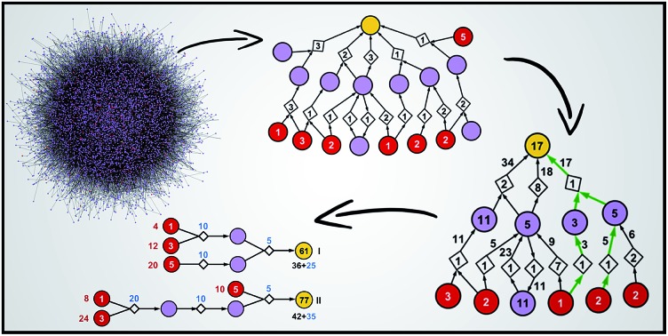
A family of network algorithms allows the Chematica retrosynthetic platform to plan both cost-effective and chemically diverse syntheses.

Abstract

As the programs for computer-aided retrosynthetic design come of age, they are no longer identifying just one or few synthetic routes but a multitude of chemically plausible syntheses, together forming large, directed graphs of solutions. An important problem then emerges: how to select from these graphs and present to the user manageable numbers of top-scoring pathways that are cost-effective, promote convergent vs. linear solutions, and are chemically diverse so that they do not repeat only minor variations in the same chemical theme. This paper describes a family of reaction network algorithms that address this problem by (i) using recursive formulae to assign realistic prices to individual pathways and (ii) applying penalties to chemically similar strategies so that they are not dominating the top-scoring routes. Synthetic examples are provided to illustrate how these algorithms can be implemented – on the timescales of ∼1 s even for large graphs – to rapidly query the space of synthetic solutions under the scenarios of different reaction yields and/or costs associated with performing reaction operations on different scales.

Introduction

Recent years have witnessed the revival of interest in computer-assisted retrosynthetic planning, which has been an elusive goal since the late 1960s.1–11 With foundational work on the representation of large collections of chemical reactions as networks12–14 and the so-called bipartite graphs15–18 and with modern hardware and algorithms allowing for rapid searches for synthetic pathways, synthetic planning by computers has finally become a tangible possibility. Indeed, several software platforms7–11,19,20 have been developed differing in the details of search algorithms and also in the origin of synthetic rules (expert-coded19,20 based on reaction mechanisms vs. automatically extracted from the literature7–11). The year 2018 also marked the first demonstration20 – on our Chematica platform – of autonomous computer design and subsequent experimental validation of multiple efficient syntheses leading to medicinally important targets. Despite this undeniable progress, however, several challenges remain and need to be considered, especially if the programs are to be adopted by practicing organic chemists. One of the challenges we consider here is how to present to the program's user synthetic solutions that are not only viable but also economical and chemically diverse.

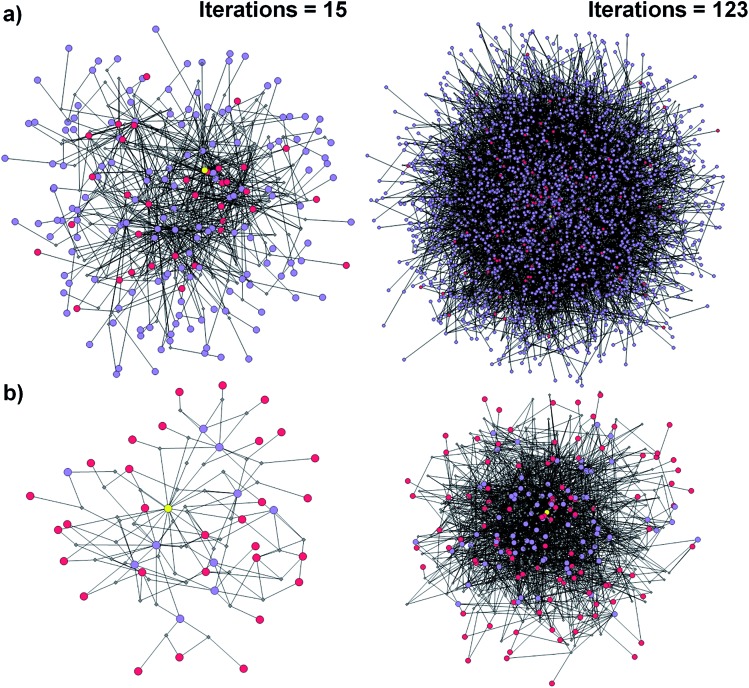
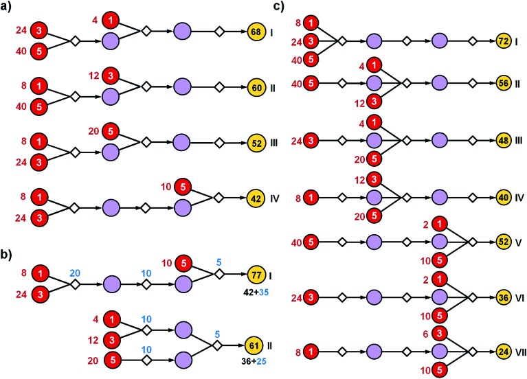
In the early stages of its development, Chematica was able to identify relatively small numbers of viable syntheses which were often variations of a similar synthetic theme. With the increasing knowledge base of reactions and with improved algorithms for the exploration of synthetic options,19,20 however, the searches started to identify increasingly large numbers of chemically correct solutions which themselves formed large synthetic networks (cf.Fig. 1). The question then arose how to estimate and rank the realistic costs of these possible pathways, taking into account not only the absolute number of steps and the costs of starting materials but also the path structure – that is, its linearity vs. convergence, the placement of the convergence points within the pathway, or the optimal “timing” to use the most expensive reagents (see examples in Fig. 2). In addition, because organic molecules can be made in different ways and the ultimate choice of a pathway often reflects practical considerations (ranging from the availability of certain reagents or equipment to the familiarity of a given chemist with particular types of reactions/procedures), it is important to present to the user multiple choices differing in the key reactions they entail. We note that although the problems of (i) finding a desired number of the best/lowest-cost solutions within the so-called directed graphs with weighted nodes (e.g., in random time-dependent networks,21–23 transit networks,21,24,25 or reaction networks19,20,26) and also (ii) identifying qualitatively different pathways (e.g., within transportation networks27) have been individually studied in graph theory, the specific approaches are not easily extendable to realistic synthetic–organic planning (cf. Discussion in Section S3†). Curiously, neither cost effectiveness nor diversity has been addressed in the existing retrosynthetic platforms, which might explain why the relevant publications usually describe just one top-scoring solution (diversity issue) and why the published pathways are often linear rather than convergent sequences (lack of realistic treatment of costs and yields). In our earlier versions of Chematica,16,19,20 the selection algorithms were also rudimentary and the cost-calculation schemes were not only extremely slow (running for thousands of seconds for large graphs of solutions) but also did not properly capture the efficiencies of individual steps and the overall path structure (linearity vs. convergence), translating into unrealistic costs of starting materials consumed and/or reaction operations performed (cf. Section S3.1†). In light of these considerations, we see the improved approaches – reflecting true synthetic costs and operating within just seconds – described in the current paper as an important advance not only for Chematica but also for other efforts in this exciting area of research.

Fig. 1. Reaction networks/graphs inspected during synthetic searches and the subgraphs of viable solutions. (a) The graphs of all molecule nodes visited during Chematica's retrosynthetic searches for the syntheses of the triarylamine target (same as in Fig. 6). The network on the left is for the early stage of the search (15 iterations of expanding retrons into progeny synthons; overall within ∼20 s computing time on a 64-core machine) and contains 456 nodes (i.e., all molecules and reactions considered during the search). The graph on the right is later in the search (123 iterations within <2 min of computing time on a 64-core machine) and contains 5300 nodes. (b) The corresponding subgraphs of the networks from (a) contain only the viable syntheses. Note that as the search progresses, the subgraphs of solutions are themselves becoming quite complex, here increasing from 90 nodes after 15 iterations to 779 nodes after 123 iterations. Color coding of the nodes: yellow = target; violet = intermediates; red = commercially available starting materials; small gray diamonds = reaction nodes.

Fig. 2. Effects of path structure on the cost of syntheses. The schemes illustrate hypothetical synthetic plans in which 1 mmol of the final product (yellow nodes on the right) is made from the same substrates (red nodes with prices per mmol given by the white numbers, i.e., 1, 3 or 5 of some currency). All syntheses use three reactions. The reaction operations in this bipartite representation are indicated by small diamond nodes and are assumed to proceed in 50% yield each. Intermediates are denoted by violet circles. Black numbers within yellow circles give the calculated cost of making 1 mmol of the target while red numbers next to the substrate nodes are costs of the starting materials that need to be used for this purpose. (a) More expensive substrates should be introduced later in the synthesis. Here, placing the substrate with cost “3” at the second step (II) lowers the cost of materials needed for the synthesis of 1 mmol of the target from 68 to 60. Likewise, as the substrate with cost “5” is introduced in the first (I), the second (III), or the third step (IV), the overall cost is progressively lowered, from 60 to 52 to 42. (b) The realistic overall cost of synthesis should also incorporate the cost of reaction operations per some unit scale (here “5” for making 1 mmol of a given reaction product). Blue numbers next to reaction nodes denote the scale required for each 50%-yield reaction to ultimately produce 1 mmol of the target. Given this 50% yield of each step and with reference to the optimal solution (IV) from panel (a), 4 mmol of the product of the first step has to be prepared (cost 5 × 4 = 20), 2 mmol of the product of the second step (cost 5 × 4 = 10), and ultimately 1 mmol of the target (cost 5 × 1 = 5). Overall, the cost of the pathway is 77 and is the sum of materials' costs (42) and reaction operations' cost (35). In contrast, with the same yields, the more convergent approach marked as (II) reduces both the labor cost (25 vs. 35) and the cost of starting materials (36 vs. 42). (c) A multicomponent reaction (MCR) used en route to a given target offers most significant cost savings if this “convergence point” is placed later within the pathway and when it uses the most expensive substrates. Here, these conditions are met for (VII).

Computer-assisted retrosynthetic searches rely on iterative expansion of the parent/retron nodes into daughter/synthon nodes and on navigating the thus-created synthetic space (with the help of various scoring functions) to ultimately reach simple and commercially available substrates. Since the search procedures are not the subject of our current work (for details, see ref. 9, 19 and 20), the starting point for our analyses is an already existing large graph of molecules considered/“visited” during synthetic planning. In a more technical parlance, we consider a large directed bipartite graph (Fig. 1a) composed of two types of nodes: molecules represented in all figures as circular nodes and reactions represented as smaller diamond-shaped nodes. The molecule nodes are of three types: the target (marked yellow in the figures), its progeny nodes (in specific chemical examples in Fig. 6–10 colored green if a molecule is known in the literature19,20 and violet otherwise) corresponding to synthetic intermediates, and commercially available starting materials (red). To enable meaningful cost estimates of the synthetic pathways, the starting materials must have realistic prices standardized to a certain common quantity – in Chematica, there are over 200 000 such nodes from the Sigma-Aldrich catalog and their prices are all standardized to “per gram,” which is easily convertible to “per mmol” we use here. The reaction nodes carry with them some “fixed cost” of performing a reaction operation r to obtain some unit quantity of the product – this cost can be loosely construed as a cost of labor plus equipment/solvent/purification and does not yet account for the prices of specific substrates and/or reaction yield that are considered only when evaluating specific pathways. The algorithms we describe below do not change if the “fixed costs” are the same or different for different reaction types (as in the example in Fig. 3). Finally, the reactions are assumed to proceed with a certain yield – although yields of each reaction in the network can be estimated individually (by machine-learning28 or by thermodynamic models29), we assume here, without losing generality of the algorithms, that the yields of all reactions in the graph are the same. In Chematica, the specific value of such a “global”/average yield can be set by the user allowing him/her to query the graph of synthetic solutions under different yield scenarios.

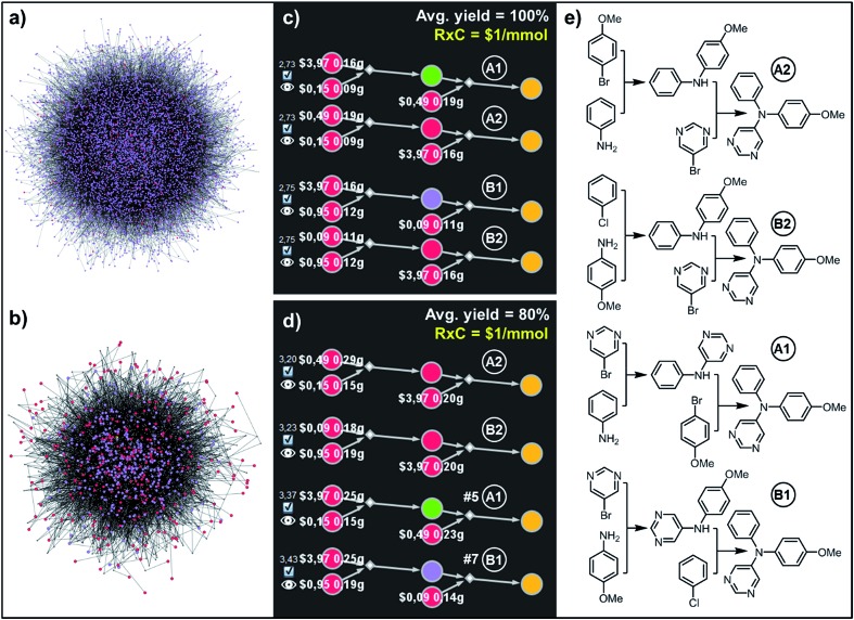
Fig. 6. Top-scoring syntheses of unsymmetrical triarylamine31 proposed by Chematica under different yield scenarios. (a) Full graph searched during the retrosynthetic planning and (b) the solution graph. (c) Chematica's screenshots of the four top-scoring syntheses obtained with yields of all steps set to 100%. (d) Ordering of these top-scoring solutions changes when the yield is set to a more realistic 80%. (e) Chemical details of the pathways. The top scoring pathway A2 is identical to the one performed experimentally in ref. 31. For further details including reaction conditions proposed by Chematica, see the ESI, Section S4.† In (c and d), RxC specifies the fixed cost of performing each reaction on a 1 mmol scale ($1) while the color coding of the nodes in Chematica's pathway miniatures is as follows: yellow = target; green = intermediates whose syntheses have been already reported in the literature and are stored in the Network of Organic Chemistry, NOC;12,14 violet = intermediates not known in the NOC; red = starting materials commercially available from Sigma-Aldrich. Pairs of white numbers over the starting materials specify the costs and amounts of these starting materials necessary to make 1 mmol of the target.

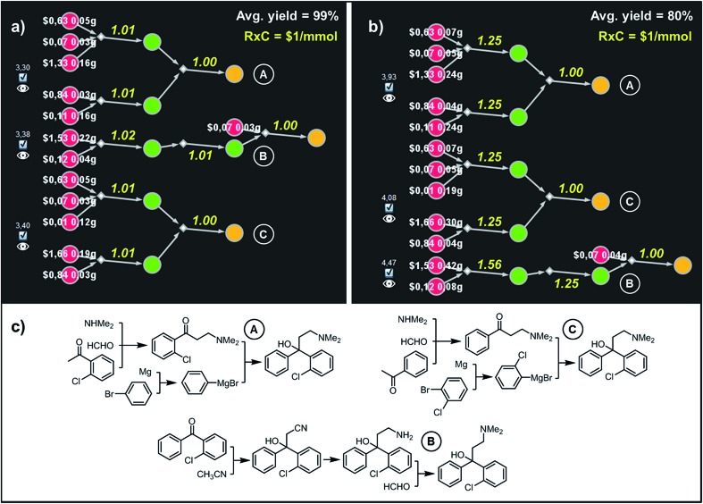
Fig. 7. Top-scoring syntheses of Clofedanol proposed by Chematica under different yield scenarios. (a) Chematica's screenshots of the three top-scoring syntheses obtained with yields of all steps set to 99%. (b) Ordering of these top-scoring solutions changes when the yield is set to a more realistic 80%. (c) Chemical details of the pathways. RxC specifies the fixed cost of performing each reaction on a 1 mmol scale ($1). Yellow numbers over reaction arrows are fixed costs rescaled to the scale required to ultimately make 1 mmol of the target. Colors of the nodes and all legends are explained in the caption to Fig. 6. For further details including reaction conditions suggested by Chematica, see the ESI, Section S5.† .

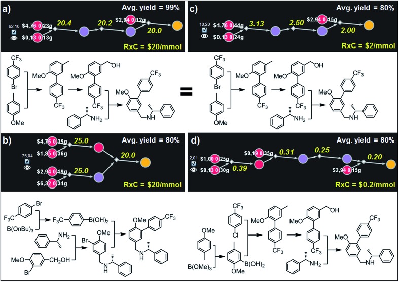
Fig. 8. Top-scoring syntheses of AMG641 proposed by Chematica under different yield and reaction-cost scenarios. Chematica's miniatures and the pathways shown below them were selected from the solution graph (created in 7 min of retrosynthetic planning; 5363 nodes in total) assuming the following values of parameters: (a) Y = 99%, RxC = $20; (b) Y = 80%, RxC = $20; (c) Y = 80%, RxC = $2; (d) Y = 80%, RxC = $0.2. Yellow numbers over reaction arrows are fixed reaction costs rescaled to the scale required to ultimately make 1 mmol of the target. Pairs of white numbers over the starting materials specify the costs and amounts of these starting materials necessary to make 1 mmol of the target. Colors of the nodes are explained in the caption to Fig. 6. For further details including reaction conditions suggested by Chematica, see the ESI, Section S6.† .

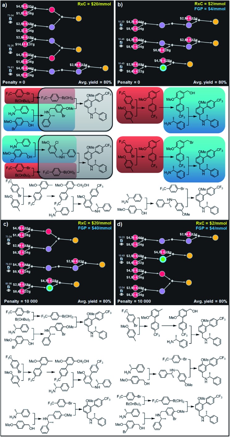
Fig. 9. Top-scoring syntheses of AMG641 proposed by Chematica without and with the application of diversity penalties. Chematica's sets of solutions shown in (a and b) have several identical (red) or very similar (blue and grey) steps when the pathways are selected from the solution graph with no penalty for reuse of already used reactions. When such a penalty is added (c and d) diversity of the synthetic plans returned is improved and each transformation is used only once. FGP is the cost of reactions requiring protection (of substances whose nodes are surrounded by blue halos). In Chematica, the cost of protection is set by the user, typically at twice the cost of reactions not requiring protection (here, FGP = 2 RxC). For further details including reaction conditions suggested by Chematica, see the ESI, Section S7.† .

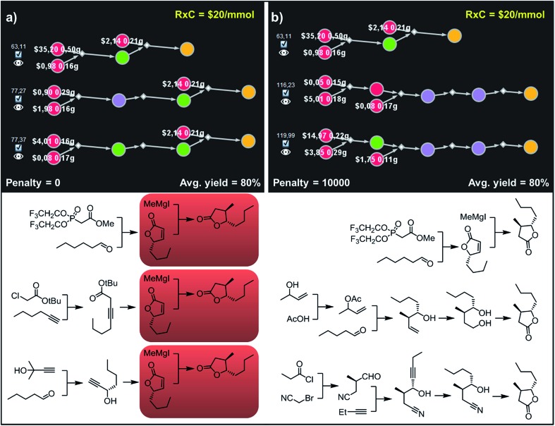
Fig. 10. Top-scoring syntheses of trans whisky lactone proposed by Chematica without and with the application of diversity penalties. (a) Without any diversity penalties, all pathways use the same method to install the C3 stereocenter (red frames). (b) When P = 10 000 penalties are imposed, all three top-scoring plans are substantially different and rely on different methodologies. For further details including reaction conditions suggested by Chematica, see the ESI, Section S8.† .

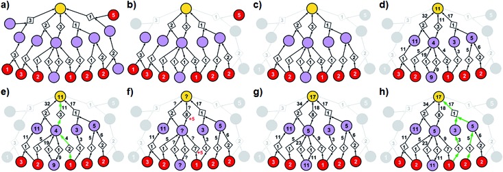
Fig. 3. Stages of selecting cost-effective yet diverse pathways from a synthetic graph. Parameters used are 50% yield for all reactions and penalty P = 5. (a) A hypothetical chemical reaction network created during a retrosynthetic search. Hypothetical costs of substrates per mmol are given over red nodes and fixed costs of reaction operations are indicated inside the diamond-shaped reaction nodes. Note that not all pathways terminate in commercially available starting materials (red nodes) as the search algorithm visited/probed some intermediates that did not lead to complete synthetic solutions. Such nodes and the pathways they are involved in are removed from consideration in (b) and (c). (d) The costs of all nodes in the remaining subgraph are computed by propagating from starting materials to the target as described in detail in the main text (see also Fig. 4). (e) The lowest-cost synthesis of the target is selected and here indicated in green. (f) Penalty P is added to the reactions from the selected pathway (here, P = +5, red numbers). Nodes whose costs increase due to such penalization are marked with question marks and are recalculated as in (g). The new “best” synthetic pathway is selected in (h) and the penalization-selection cycle can be again repeated as needed.

Results and discussion

Scoring and selecting cost-optimal pathways

With algorithmic details described in the ESI, Section S1,† the general procedure for pathway selection is illustrated in Fig. 3. Within the initial network in Fig. 3a, we define (i) chemical nodes as “synthesizable” if they are targets of at least one synthetic pathway tracing back to commercially available substrates and (ii) reaction nodes as “viable” if all their substrates are synthesizable. In the first step, the algorithm finds all synthesizable nodes in the network in a depth-first-search-like manner and using the fact that a chemical is synthesizable only if it is commercially available or is a product of some viable reaction. If the target is not among the synthesizable nodes, then the selection algorithm stops without returning any pathways. Otherwise, it proceeds as follows. A subgraph of the network induced by synthesizable nodes is computed and retained (Fig. 3b). This step removes all substance nodes that are not synthesizable and reactions that are not viable. Then, the remaining subgraph is further restricted to one induced by ancestors of the target and the target itself (Fig. 3c). This step removes nodes which do not belong to any pathways leading to the target. Over the remaining subgraph, called the solution graph, the cost of each chemical node is taken as the smallest cost of all syntheses that can produce this chemical. The cost of any reaction node in the network is the smallest cost of all synthetic pathways containing this particular reaction and giving this reaction product. Accordingly, for each non-starting-material chemical, c, in the network, its cost is prescribed recursively by cost(c) = min_r∈pred(c)(cost(r)), while for each reaction node we have , where fixed_cost(r) was discussed in the preceding paragraph (cost of performing synthetic operations on some unit scale) and pred denotes the set of predecessors of a given node in the network. In the subsequent step, the costs of all nodes in the network are calculated bottom-up (i.e., from the starting materials to the target) using a Dijkstra-like algorithm similar to the one for finding minimum-weight B-paths in weighted hypergraphs24 (see also ref. 26).

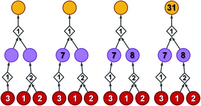
To illustrate how these operations work, let us first consider a simple tree in Fig. 4 in which each of the intermediates can be made in only one way and all reactions have, say, 50% yield. For the left branch, the substrate with price “3” enters in the reaction with a fixed cost of “1”. Because of the 50% yield, making 1 mmol of this reaction product requires 2 mmol of the substrate, and the total reaction cost is 1 + 3/50% = 7. For the reaction in the right branch, the unit cost is different (“2”; this reaction may be just harder to perform experimentally) but the cost calculation is analogous, 2 + (1 + 2)/50% = 8. These costs are assigned to the intermediates and propagated to the target in another 50%-yield reaction – the overall cost of making 1 mmol of the target will be 1 + (7 + 8)/50% = 31. The result of this recursive procedure agrees with the overall chemical balance – indeed, to make 1 mmol of the target, we used 4 mmols of each substrate (cost 4 × 3 + 4 × 2 + 4 × 1 = 24) and performed the initial two reactions (from the substrates) on twice the scale of the final reaction making the target – hence, the cost of reaction operations is (2 × 1 + 2 × 2) + 1 × 1 = 7 and the total cost of making 1 mmol of the target is 24 + 7 = 31. We note that such calculations can be performed rapidly for arbitrary graphs including those that contain cycles (see the small cycle involving the violet node in the bottom row of networks in Fig. 3) – the cycles, however, are chemically unproductive and the costs they entail are always higher than for acyclic pathways (compare the costs of paths 1 → 4 vs. 1 → 4 → 9 → 4 in Fig. 3d).

Fig. 4. A simple example illustrating bottom-up propagation of costs. All reactions have the same yield of 50%. Costs of starting materials (per mmol) are given by the numbers in the red nodes. Fixed costs of synthetic operations are indicated inside the diamond-shaped reaction nodes. For details of the calculations, see the main text.

Coming back to Fig. 3d, we observe that in realistic networks, there is generally more than one pathway to make a given chemical – for instance, the second-from-the-left intermediate can be made in three ways, via reactions with costs of 5, 19, and 4. Of these, we chose the least expensive option and assign to the intermediate the cost of 4, as prescribed by the formula cost(c) = min_r∈pred(c)(cost(r)). Having scored all nodes within the graph, we then easily identify the most cost-effective pathway by subsequent choices (from target “down”) of the lowest-scoring reactions at each synthetic generation (in our example, “11” followed by “4”; Fig. 3e). The information about other pathways (i.e., their fragments and estimated costs) is kept in a priority queue, like in an A* algorithm, and the graph is re-searched via a greedy-descent-type algorithm to find the second, third, etc. best pathways (see algorithmic details in the ESI, Section S1.4†).

Note that if one wishes to find pathways composed of minimal numbers of steps – which is a common situation in small-scale pharmaceutical synthesis whereby time is of essence and one might not even care about the prices of substrates or yields but just focus on synthesizing the target as rapidly as possible in amounts adequate for the upcoming assays – then the algorithm's parameters should be set to 100% yields, zero cost for all starting materials, and all fixed costs set to some common value. Under such assumption, the overall pathway score is simply the sum of the fixed_cost(r) over all r's (with the exception of some pathways which are not trees; see ESI, Section S1.1†). In another limiting case, when the fixed costs (labor costs) are negligible (fixed_cost(r) = 0), the cost is equal to the total cost of starting materials needed to synthesize 1 mmol of the target (taking into account the loss of mass for realistic yields <100%). The full scoring scheme we consider takes into account not just the number of steps (through the fixed_cost cost term) or costs of starting materials but also both of these factors simultaneously along with yields and most optimal placement of convergence points within a pathway.

Assigning penalties and ensuring synthetic diversity

The selection algorithm described so far can return n best-scoring pathways but does not guarantee in any way that these pathways are structurally diverse. For instance, two top-scoring solutions for the synthesis of triarylamine in Fig. 6d rely on the key Buchwald–Hartwig-type amination of the bromopyrimidine and differ only in the method of preparation of the diarylamine. In the same spirit, negligible modifications such as changing an aryl bromide to an iodide are formally different pathways to the computer but are pretty much equivalent to a user chemist. To avoid these and other unproductive repetitions and to select cost-effective yet chemically diverse pathways, we proceed as follows. After finding the best pathway (cf. above), the algorithm repeats the following sequence of steps until it finds the requested number of pathways or discovers that there are no more pathways left in the network:

(i) A penalty P is added to the fixed costs of each reaction from the most-recently-found pathway (Fig. 3f) and, to avoid reusing similar synthetic solutions in other pathways, also to other reactions in the network that have the same product and non-trivial (i.e., having at least four carbon atoms) substrates;

(ii) A depth-first-search-like algorithm is used to identify the nodes (both reaction and molecule nodes) whose cost is affected due to the newly imposed penalization (nodes marked with question marks in Fig. 3f);

(iii) The costs of all affected nodes are recalculated by a modified Dijkstra algorithm (Fig. 3g);

(iv) Finally, a new lowest-cost pathway is identified and cycles (i)–(iv) are repeated. For all other algorithmic details, see the ESI, Sections S1.5 and S1.6.†

Algorithms' performance

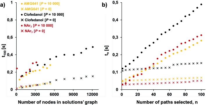
One of our key motivations for developing the selection and diversity routines has been to allow queries of the solution space on timescales much shorter than those involved in the initial retrosynthetic planning creating this space. During retrosynthetic planning, Chematica has to perform multiple operations ranging from relatively rapid matching of the reaction-rule templates (such matching is common to all retrosynthesis platforms) to much slower and Chematica-peculiar assignments of proper stereo- and regiochemistry, calculations of electronic populations for some reaction types, and several more (for details, see ref. 19, 20 and 30). In effect, searches for the solutions take from minutes for medicinal-chemistry targets to hours for complex natural products, in the end presenting to the user a given number (on the order of 100) of top-scoring solutions and, at this point, discarding the remaining ones. Retaining (e.g., saving on disk) the entire space of solutions allows the user to query it multiple times under different scenarios (costs of reactions, average yields, and magnitudes of imposed diversity penalties). Importantly, querying a solution graph does not involve all the slow routines of retrosynthetic planning and should thus be possible on much shorter time scales – indeed, typical times for assigning costs and selecting pathways are on the order of 1 s, even for large solution graphs and for different target molecules. Specifically, Fig. 5a shows the times t₁₀₀ to select (on a machine with 2.5 GHz AMD Opteron 6380 processors) 100 lowest-cost pathways from solution graphs ranging in size from 90 to ca. 12 000 nodes – these solution graphs are for the actual synthetic examples we discuss later in the text (triarylamine, Fig. 6; Bayer's Clofedanol, Fig. 7; Amgen's AMG641 modulator of the calcium sensing receptor, Fig. 8). As seen, these t₁₀₀ times are on the order of 0.25 s without any diversity penalties and ∼0.5 s when diversity penalties P are added and costs of nodes need to be recalculated as new pathways are being selected. We note that the times to select n lowest cost pathways, t_n, scale approximately linearly with n and are also below 0.5 s for the largest solution graphs (Fig. 5b).

Fig. 5. Typical times to select pathways from the solution graphs. (a) Times t₁₀₀ to select 100 lowest-cost pathways from graphs of different sizes (graph size increases as the search algorithm identifies new solutions); (b) times t_n to select n lowest-cost pathways from the maximum-size solution graphs considered here (∼3000 nodes for triarylamine from Fig. 6; ∼12 000 nodes for Bayer's Clofedanol from Fig. 7; and ∼5400 nodes for Amgen's AMG641 modulator of the calcium sensing receptor from Fig. 8). Cross markers are for selection without diversity penalty P; solid circles are for selection with penalty P = 10 000.

Illustrative synthetic examples

To illustrate how the above procedures work in practice, we considered several realistic synthetic-design examples in which the solution graphs were created by Chematica within 2–10 minutes using its standard scoring functions (see ref. 19 and 20) and comprised pathways terminating in commercially available starting materials (with prices in USD per gram, converted by the program to per mmol). We queried the solution graphs varying the average yields, the fixed costs of individual reactions on a 1 mmol scale, and the diversity penalties (henceforth denoted, respectively, Y, RxC, and P).

(i) Pathway ordering under various yield scenarios

In the first example, Chematica designed routes to an unsymmetrical triarylamine used previously in the context of photochemical synthesis of complex carbazoles in continuous flow.31 Within ca. 2 min the program searched the graph of 17 881 nodes (6826 intermediates, 293 starting materials, and 10 761 reactions; Fig. 6a), from which a solution graph composed of 3176 nodes (392 intermediates, 293 starting materials, and 2490 reactions) was selected (Fig. 6b). When this solution graph was queried with the fixed cost of each reaction operation per mmol, RxC = $1, and with an average yield of Y = 100% – that is, naively omitting mass losses at each step – the costs of the top-scoring pathways in Fig. 6c and e were simple sums of costs of performing reactions (here, $1 per mmol step × 2 steps = $2 per mmol) plus the costs of starting materials. While all these solutions, relying on Buchwald–Hartwig amination, were chemically correct, the algorithm was not able to capture the differences in the costs of various starting materials being used in the first vs. second steps. In particular, the costs of syntheses utilizing the most expensive reagent, bromopyrimidine, in the first (A1) vs. the second steps (A2) were exactly the same (“$2.73,” numbers to the left of the pathways in Fig. 6c), which is in contrast to the considerations from Fig. 2 showing that most expensive substrates should come in “closer to the target”. This problem was avoided by specifying a more realistic average yield (Y = 80%, close to the average yield of all known reactions, see ref. 28) such that the pathway costs now reflected mass loss at each step – under this condition, the top-scoring pathways A2 and B2 (Fig. 6d and e) used the expensive bromopyrimidine in the second step. We note that the top-scoring pathway A2 was actually validated experimentally in ref. 31 which inspired this example.

In the second example, more relevant to pharmaceutical chemistry, Chematica designed pathways leading to Clofedanol, a dry cough suppressant. Choosing from the solution graph created within 10 min search time and comprising 12 074 nodes in total, the cost-optimal pathways were sought with the same fixed per-mmol cost of each reaction (RxC = $1) but under two different average-yield scenarios, Y = 99% and Y = 80%. Under the first scenario, the lowest-cost pathway – marked as (A) in Fig. 7 – commences with the three component Mannich reaction of 2-chloroacetophenone, followed by addition of phenylmagnesium bromide to the obtained ketone. This solution resembles the route patented in 2009 by Zhejiang Hisoar Pharma.32 The second-scoring synthetic plan, (B), starts with the addition of acetonitrile to appropriate benzophenone, reduction of the nitrile to an amine, and reductive dimethylation with formaldehyde. This strategy is, in fact, the same as the method of preparation described in Bayer's initial (1962) patent covering Clofedanol.33 Finally, the third-best solution, (C), also relies on the Mannich reaction of acetophenone, followed by the addition of Grignard reagent derived from o-bromochlorobenzene.34 In contrast, when the average yield is Y = 80%, Bayer's pathway is disfavored. In re-evaluating it, the algorithm recalculates the amounts and costs of necessary starting materials (e.g., one now needs 0.42 g of benzophenone vs. 0.22 g under 99%-yield assumption) and scales the costs of performing synthetic steps on larger scales (compare yellow numbers in Fig. 7a and b; e.g., the addition of acetonitrile to benzophenone must now yield over 1.5 mmol of the adduct if 1 mmol of Clofedanol is expected at the end). Consequently, pathway (B) appears to be less economically feasible and is ranked lower than both approaches taking advantage of the Mannich reaction. Of course, when making such comparisons in industrial reality, it would be essential to use substrate catalogs with wholesale prices available to a specific organization, not catalog prices of Sigma-Aldrich focusing on the sales of small quantities of specialty chemicals. Fortunately, connecting a requisite catalog to Chematica or any other retrosynthetic program is a technically trivial task.

(ii) Pathway ordering under various yield and fixed-reaction-cost scenarios

The example in this section is intended to illustrate how the optimal pathways vary when both the average reaction yields and the fixed costs of performing individual reactions on a given scale change. Specifically, we query the graph of synthetic solutions leading to Amgen's AMG641 (ref. 35) – an orally efficacious, positive allosteric modulator of the calcium sensing receptor – varying Y from 99% down to 80% and RxC from $20 (expensive, probably small-scale synthesis) to $0.2 (relatively inexpensive, probably larger scale production). For Y = 99% and RxC = $20, the best-scoring solution in Fig. 8a is a three step linear sequence initialized by an elegant one-pot ortho-lithiation/Pd-mediated coupling36 with 4-trifluoromethylbromobenzene; subsequent oxidation of the benzylic position37 and alkylation of commercially available chiral amines yield the target molecule. When reaction costs remain the same but one accounts for the mass loss at each step (Y = 80%; Fig. 8b), the best solution is a convergent three-step sequence, mirroring the original Amgen's route and using benzylic alcohol to alkylate the amine in one-pot oxidation-reductive amination38 and boronic acid (prepared in one step from appropriate bromoarene) to construct the biphenyl part of AMG641.

Although both of these routes are chemically correct, they might not be optimal if AMG641 goes into large-scale production characterized by lower reaction-operation costs (e.g., achieved by solvent recycling, use of crystallization rather than chromatography, etc.). To emulate such hypothetical scale-up, we kept Y = 80% but decreased RxC to $2 and then to $0.2. In the first case, the best-scoring solution (Fig. 8c) is actually the same as in Fig. 8a for Y = 99%. We note, however, that the overall cost of this plan recalculated with Y = 80%, RxC = $2 constrains is, as expected, very different ($10.2 per mmol vs. $62.1 per mmol in Fig. 8a), reflecting slightly higher quantities and costs of starting materials ($2.56 vs. $1.38) but much lower costs of reaction operations (7.63$ vs. 60.6$). Finally, further decrease of RxC to $0.2 adds an extra step (labor/operations are now cheap!) but sources the synthesis from very inexpensive starting materials (4-methylanisole and chloroarene). This four step linear sequence is shown in Fig. 8d and begins with the Suzuki coupling of aryl chloride and boronic acid prepared via ortho-lithiation and trapping of the obtained aryllithium with trimethyl borate. Subsequent oxidation of the benzylic position and junction with an appropriate amine leads to the target molecule. Taken together, the examples we discussed in this section illustrate that by varying the Y and RxC parameters, the machine makes pathway selections that reflect the economical differences between medicinal chemistry and manufacturing operations.

(iii) Selection of diverse pathways

The pathways we described in previous examples were all chemically viable and the selection algorithm adapted to different scoring/pricing scenarios, but within each scenario, the variability among the n best-scoring pathways was far from satisfactory – in other words, the n top-scoring pathways selected for given values of Y and RxC could rely on the same or chemically equivalent transformations. This limits the menu of solutions the user is presented with. To illustrate the problem and how to remedy it by imposing penalties P on the reuse of equivalent transforms (see Fig. 3 and accompanying algorithm described earlier in the text), we required that Chematica returns three top scoring syntheses of the AMG641 target under the two Y–RxC scenarios from Fig. 8b,c but with vs. without diversity penalization. With no penalization (P = 0) the selection algorithm proposed sets of synthetic plans in which the same or similar transformations were used several times. For example, the first and second solutions shown in Fig. 9a (Y = 80%, RxC = $20 per mmol) rely on the Suzuki coupling of p-trifluoromethylbenzeneboronic acid with either bromo- or chloroarene (grey). Additionally, the necessary haloarene is prepared via alkylation of the same benzylamine with either appropriate bromobenzyl bromide or chlorobenzyl alcohol (blue) while the preparation of the boronic acid in both plans starts from the same bromobenzene (red) undergoing Br/Li exchange and trapping with tributyl borate. Similar redundancy was observed in results obtained under different Y–RxC scenarios (Y = 80%, RxC = $2 per mmol) and is illustrated in Fig. 9b. Here, the only minor difference between the top and the second-best solutions is, in fact, the leaving group of the benzylating agent used in the N-alkylation. In both pathways, the last step (blue) requires the same amine undergoing alkylation while the construction of the biphenyl part of AMG641 takes advantage of the identical lithiation–arylation (red). In sharp contrast, results obtained after applying large diversity penalty (P = 10 000) are chemically diverse. In particular, sets of synthetic plans shown in Fig. 9c and d rely on the (i) alkylation of the amine with the m-bromobenzyl alcohol and subsequent Suzuki coupling, (ii) ortho-lithiation/arylation, followed by hydroxylation and N-alkylation, or (iii) alkylation of the amine with p-methoxybenzyl alcohol and late-stage lithiation/arylation. All of the transformations used in these sets of plans are unique and used only once in the entire series of solutions – though, we observe, these relatively simple syntheses still bear some “thematic” similarity.

Accordingly, to allow for more synthetic latitude and diversity, our final example deals with more complex enantioselective syntheses of trans-whisky lactone (3-methyl-4-octanolide) isolated from oak wood and responsible for the taste of aged spirits.39 With no penalization applied (P = 0) each of the three top-scoring synthetic plans relies on the formation of butenolides and subsequent trans-selective 1,4-addition of organocuprate (derived from methylmagnesium iodide; Fig. 10a, red frames) to set the C3 stereocenter, mimicking previous literature approaches.40,41 The necessary enantioenriched butenolide can be obtained from hexanal via proline-mediated aminoxylation-olefination42 (Fig. 10a, top path). We note that this approach was demonstrated experimentally during preparation of the structurally similar trans-cognac lactone.42 Alternatively, the butenolide can be prepared via enantioselective isomerization-cyclisation43 of β,γ-alkynoic ester which is available in one step from hexyne and chloroacetate (Fig. 10a, middle), or via enantioselective addition44 of protected acetylene to pentanal, followed by carbonylative cyclisation45,46 (Fig. 10a, bottom). In contrast, after applying diversity penalty (P = 10 000), the alternative pathways no longer hinge on the 1,4-addition and both contiguous stereocenters are forged prior to the formation of the lactone. In particular, the second-best solution (Fig. 10b, middle path) now takes advantage of the Krische's crotylation47 of pentanal setting both stereocenters. Hydroboration of the homoallylic alcohol thus obtained yields a 1,4-diol undergoing oxidative cyclisation48 to the target molecule. Finally, the third-plan (Fig. 10b, bottom) commences with a chiral-auxiliary-controlled cyanomethylation of the enolate with bromoacetonitrile.49 Subsequent addition of butynal controlled by a chiral catalyst50,51 yields hydroxynitrile, which then undergoes reduction of alkyne and intramolecular alcoholysis to the whisky lactone target.

Conclusions

In summary, we described a family of algorithms that select and score the most economical and diverse synthetic pathways from large graphs of synthetically viable solutions. This problem has not been addressed in detail in previous literature on computer-assisted retrosynthesis likely because – until now – few solutions were produced during retrosynthetic searches and any chemically viable outcome has been deemed a success. Now, with much improved algorithms and modern computing power, the situation has changed and one faces the embarras de richesse problem, with very large numbers of potential solutions, all chemically plausible. With the algorithms like the ones we described, one can save the entire solution space and then query it rapidly, within seconds, for pathways meeting desired cost scenarios (instead of re-running the slow retrosynthetic search with different parameters). As we mentioned in the text, to truly reflect the realistic costs of specific organizations, the algorithm should be interfaced with catalogs of starting materials with prices peculiar to these organizations. In the future, one could also think of augmenting the penalization schemes – here, used to ensure chemical diversity – to downplay the use of reagents that are undesirable (toxic, volatile, etc.) or reaction types known to be particularly difficult or finicky.

Author contributions

T. B. designed and implemented the selection algorithms. K. M. validated the algorithms for synthetic correctness and provided examples of syntheses described in the text. B. A. G. conceived Chematica in graduate school and has directed the development of its various aspects – including the current work – ever since. All authors contributed to the writing of the manuscript.

Conflicts of interest

While Chematica was originally developed and owned by B. A. G.'s Grzybowski Scientific Inventions, LLC, neither he nor the co-authors currently hold any stock in this company, which is now a property of Merck KGaA, Darmstadt, Germany. The authors continue to collaborate with Merck KGaA, Darmstadt, within the DARPA “Make-It” award. All queries about access options to Chematica (now rebranded as Synthia™), including academic collaborations, should be directed to Dr Sarah Trice at Email: sarah.trice@sial.com.

References

- Corey E. J., Wipke W. T. Science. 1969;166:178–192. doi: 10.1126/science.166.3902.178. [DOI] [PubMed] [Google Scholar]
- Corey E. J., Wipke W. T., Cramer R. D., Howe W. J. J. Am. Chem. Soc. 1972;94:421–430. [Google Scholar]
- Corey E. J., Wipke W. T., Cramer R. D., Howe W. J. J. Am. Chem. Soc. 1972;94:431–439. [Google Scholar]
- Gelernter H. L., Sanders A. F., Larsen D. L., Agarwal K. K., Boivie R. H., Spritzer G. A., Searleman J. E. Science. 1977;197:1041–1049. doi: 10.1126/science.197.4308.1041. [DOI] [PubMed] [Google Scholar]
- Hanessian S., Franco J., Larouche B. Pure Appl. Chem. 1990;62:1887–1910. [Google Scholar]
- Hendrickson J. B. J. Am. Chem. Soc. 1977;99:5439–5450. [Google Scholar]
- Law J., Zsoldos Z., Simon A., Reid D., Liu Y., Khew S. Y., Johnson A. P., Major S., Wade R. A., Ando H. Y. J. Chem. Inf. Model. 2009;49:593–602. doi: 10.1021/ci800228y. [DOI] [PubMed] [Google Scholar]
- Bøgevig A., Federsel H.-J., Huerta F., Hutchings M. G., Kraut H., Langer T., Löw P., Oppawsky C., Rein T., Saller H. Org. Process Res. Dev. 2015;19:357–368. [Google Scholar]
- Segler M. H. S., Preuss M., Waller M. P. Nature. 2018;555:604–610. doi: 10.1038/nature25978. [DOI] [PubMed] [Google Scholar]
- Coley C. W., Rogers L., Green W. H., Jensen K. F. ACS Cent. Sci. 2017;3:1237–1245. doi: 10.1021/acscentsci.7b00355. [DOI] [PMC free article] [PubMed] [Google Scholar]
- Coley C. W., Green W. H., Jensen K. F. Acc. Chem. Res. 2018;51:1281–1289. doi: 10.1021/acs.accounts.8b00087. [DOI] [PubMed] [Google Scholar]
- Fialkowski M., Bishop K. J. M., Chubukov V. A., Campbell C. J., Grzybowski B. A. Angew. Chem., Int. Ed. 2005;44:7263–7269. doi: 10.1002/anie.200502272. [DOI] [PubMed] [Google Scholar]
- Bishop K. J. M., Klajn R., Grzybowski B. A. Angew. Chem., Int. Ed. 2006;45:5348–5354. doi: 10.1002/anie.200600881. [DOI] [PubMed] [Google Scholar]
- Grzybowski B. A., Bishop K. J. M., Kowalczyk B., Wilmer C. E. Nat. Chem. 2009;1:31–36. doi: 10.1038/nchem.136. [DOI] [PubMed] [Google Scholar]
- Gothard C. M., Soh S., Gothard N. A., Kowalczyk B., Wei Y., Baytekin B., Grzybowski B. A. Angew. Chem., Int. Ed. 2012;51:7922–7927. doi: 10.1002/anie.201202155. [DOI] [PubMed] [Google Scholar]
- Kowalik M., Gothard C. M., Drews A. M., Gothard N. A., Weckiewicz A., Fuller P. E., Grzybowski B. A., Bishop K. J. M. Angew. Chem., Int. Ed. 2012;51:7928–7932. doi: 10.1002/anie.201202209. [DOI] [PubMed] [Google Scholar]
- Fuller P. E., Gothard C. M., Gothard N. A., Weckiewicz A., Grzybowski B. A. Angew. Chem., Int. Ed. 2012;51:7933–7937. doi: 10.1002/anie.201202210. [DOI] [PubMed] [Google Scholar]
- Chaouiya C. Briefings Bioinf. 2007;8:210–219. doi: 10.1093/bib/bbm029. [DOI] [PubMed] [Google Scholar]
- Szymkuć S., Gajewska E. P., Klucznik T., Molga K., Dittwald P., Startek M., Bajczyk M., Grzybowski B. A. Angew. Chem., Int. Ed. 2016;55:5904–5937. doi: 10.1002/anie.201506101. [DOI] [PubMed] [Google Scholar]
- Klucznik T., Mikulak-Klucznik B., McCormack M. P., Lima H., Szymkuć S., Bhowmick M., Molga K., Zhou Y., Rickershauser L., Gajewska E. P., Toutchkine A., Dittwald P., Startek M. P., Kirkovits G. J., Roszak R., Adamski A., Sieredzińska B., Mrksich M., Trice S. L. J., Grzybowski B. A. Chem. 2018;4:522–532. [Google Scholar]
- Nielsen L. R., Andersen K. A., Pretolani D. Comput. Oper. Res. 2005;32:1477–1497. [Google Scholar]
- Miller-Hooks E. Networks. 2001;37:35–52. [Google Scholar]
- Pretolani D. Eur. J. Oper. Res. 2000;123:315–324. [Google Scholar]
- Gallo G., Longo G., Pallottino S., Nguyen S. Discrete Appl. Math. 1993;42:177–201. [Google Scholar]
- Nguyen S., Pallottino S. Eur. J. Oper. Res. 1988;37:176–186. [Google Scholar]
- Fagerberg R., Flamm C., Kianian R., Merkle D., Stadler P. F. J. Cheminf. 2018;10:19. doi: 10.1186/s13321-018-0273-z. [DOI] [PMC free article] [PubMed] [Google Scholar]
- Akgün V., Erkut E., Batta R. Eur. J. Oper. Res. 2000;121:232–246. [Google Scholar]
- Skoraczyński G., Dittwald P., Miasojedow B., Szymkuć S., Gajewska E. P., Grzybowski B. A., Gambin A. Sci. Rep. 2017;7:3582. doi: 10.1038/s41598-017-02303-0. [DOI] [PMC free article] [PubMed] [Google Scholar]
- Emami F. S., Vahid A., Wylie E. K., Szymkuć S., Dittwald P., Molga K., Grzybowski B. A. Angew. Chem., Int. Ed. 2015;54:10797–10801. doi: 10.1002/anie.201503890. [DOI] [PubMed] [Google Scholar]
- Beker W., Gajewska E. P., Badowski T., Grzybowski B. A. Angew. Chem., Int. Ed. 2019;58:4515–4519. doi: 10.1002/anie.201806920. [DOI] [PubMed] [Google Scholar]
- Hernandez-Perez A. C., Caron A., Collins S. K. Chem.–Eur. J. 2015;21:16673–16678. doi: 10.1002/chem.201502661. [DOI] [PubMed] [Google Scholar]
- He T. and Wenqiu Y., CN101844989, 2009.
- Lorenz R., Gosswald R. and Henecka H., US3031377A, 1962.
- Sulake R. S., Chen C., Lin H.-R., Lua A.-C. Bioorg. Med. Chem. Lett. 2011;21:5719–5721. doi: 10.1016/j.bmcl.2011.08.021. [DOI] [PubMed] [Google Scholar]
- Harrington P. E., Jean D. J. St., Clarine J., Coulter T. S., Croghan M., Davenport A., Davis J., Ghiron C., Hutchinson J., Kelly M. G., Lott F., Lu J. Y.-L., Martin D., Morony S., Poon S. F., Portero-Larragueta E., Reagan J. D., Regal K. A., Tasker A., Wang M., Yang Y., Yao G., Zeng Q., Henley C., Fotsch C. Bioorg. Med. Chem. Lett. 2010;20:5544–5547. doi: 10.1016/j.bmcl.2010.07.060. [DOI] [PubMed] [Google Scholar]
- Giannerini M., Hornillos V., Vila C., Fañanás-Mastral M., Feringa B. L. Angew. Chem., Int. Ed. 2013;52:13329–13333. doi: 10.1002/anie.201306427. [DOI] [PubMed] [Google Scholar]
- Cort A. D., Mandolini L., Panaioli S. Synth. Commun. 1988;18:613–616. [Google Scholar]
- Guérin C., Bellosta V., Guillamot G., Cossy J. Org. Lett. 2011;13:3534–3537. doi: 10.1021/ol201351a. [DOI] [PubMed] [Google Scholar]
- Otsuka K., Zenibayashi Y., Itoh M., Totsuka A. Agric. Biol. Chem. 1974;38:485–490. [Google Scholar]
- Koschker P., Kähny M., Breit B. J. Am. Chem. Soc. 2015;137:3131–3137. doi: 10.1021/jacs.5b01131. [DOI] [PubMed] [Google Scholar]
- Mao B., Geurts K., Fañanás-Mastral M., van Zijl A. W., Fletcher S. P., Minnaard A. J., Feringa B. L. Org. Lett. 2011;13:948–951. doi: 10.1021/ol102994q. [DOI] [PubMed] [Google Scholar]
- Devalankar D. A., Chouthaiwale P. V., Sudalai A. Tetrahedron: Asymmetry. 2012;23:240–244. [Google Scholar]
- Liu H., Leow D., Huang K.-W., Tan C.-H. J. Am. Chem. Soc. 2009;131:7212–7213. doi: 10.1021/ja901528b. [DOI] [PubMed] [Google Scholar]
- Boyall D., López F., Sasaki H., Frantz D., Carreira E. M. Org. Lett. 2000;2:4233–4236. doi: 10.1021/ol006791r. [DOI] [PubMed] [Google Scholar]
- Yu W.-Y., Alper H. J. Org. Chem. 1997;62:5684–5687. [Google Scholar]
- Gallagher W. P., Maleczka R. E. J. Org. Chem. 2003;68:6775–6779. doi: 10.1021/jo034463+. [DOI] [PubMed] [Google Scholar]
- Gao X., Townsend I. A., Krische M. J. J. Org. Chem. 2011;76:2350–2354. doi: 10.1021/jo200068q. [DOI] [PMC free article] [PubMed] [Google Scholar]
- Ito M., Osaku A., Shiibashi A., Ikariya T. Org. Lett. 2007;9:1821–1824. doi: 10.1021/ol0706408. [DOI] [PubMed] [Google Scholar]
- Crimmins M. T., Shamszad M., Mattson A. E. Org. Lett. 2010;12:2614–2617. doi: 10.1021/ol1008203. [DOI] [PMC free article] [PubMed] [Google Scholar]
- Marshall J. A., Bourbeau M. P. Org. Lett. 2003;5:3197–3199. doi: 10.1021/ol034918h. [DOI] [PubMed] [Google Scholar]
- Takita R., Yakura K., Ohshima T., Shibasaki M. J. Am. Chem. Soc. 2005;127:13760–13761. doi: 10.1021/ja053946n. [DOI] [PubMed] [Google Scholar]
Associated Data
This section collects any data citations, data availability statements, or supplementary materials included in this article.