Improving the time‐machine: estimating date of birth of grade II gliomas

Abstract

Objectives:  Here we present a model aiming to provide an estimate of time from tumour genesis, for grade II gliomas. The model is based on a differential equation describing the diffusion–proliferation process. We have applied our model to situations where tumour diameter was shown to increase linearly with time, with characteristic diametric velocity.

Materials and methods:  We have performed numerical simulations to analyse data, on patients with grade II gliomas and to extract information concerning time of tumour biological onset, as well as radiology and distribution of model parameters.

Results and conclusions:  We show that the estimate of tumour onset obtained from extrapolation using a constant velocity assumption, always underestimates biological tumour age, and that the correction one should add to this estimate is given roughly by 20/v (year), where v is the diametric velocity of expansion of the tumour (expressed in mm/year). Within the assumptions of the model, we have identified two types of tumour: the first corresponds to very slowly growing tumours that appear during adolescence, and the second type corresponds to slowly growing tumours that appear later, during early adulthood. That all these tumours become detectable around a mean patient age of 30 years could be interesting for formulation of strategies for early detection of tumours.

Introduction

This article is devoted to the study of grade II gliomas. To fix the frame of our investigations, we have needed to refer to World Health Organization (WHO) classification, according to which, gliomas are classified with respect to their malignancy from grades I to IV (1). Grade II gliomas we shall deal with in this article correspond to diffusely infiltrative tumours that are incurable. Initially, grade II gliomas are characterized by slow tumour growth and by infiltration of brain parenchyma by isolated tumour cells (2, 3). Inevitably, anaplastic cell changes occur, jeopardizing both functional and vital prognoses for the patient, despite surgery, chemotherapy or radiotherapy (4, 5, 6, 7, 8, 9, 10). Danger of diffuse tumours lies in the fact that tumour cells migrate well beyond the bulk detected by imaging techniques (11). Several modelling approaches have undertaken to account for migration of cells and their effect on tumour expansion (12, 13, 14, 15, 16, 17). For example, in (18, 19, 20, 21), a cellular automaton and its continuous limit were initially used to describe cell migration, having interactions with other tumour cells and with normal cells of their substrate. However, a more sophisticated model has recently been proposed (22). Here, the authors have introduced a hybrid model, consisting of a continuum (for description of tumour body growth), and a discrete portion (for description of cell propagation and interaction). Merits of such a model are that it minimizes computational burden of the discrete portion, small calculations, without eschewing them altogether, and thus describing in as realistic as possible way, the cell migration process.

Another approach is to conceive a minimal model, based on a partial differential equation, featuring the two main phenomena determining evolution of the tumour, that is, proliferation and cell movement. It was in this context that mathematical, spatiotemporal models were introduced (23, 24, 25, 26, 27). The basic model posits that the concentration of glioma cells varies in time with a rate given by the result of cell diffusion and cell proliferation. Formally, the equation assumes the form:

(1)

where is glioma cell concentration, κ proliferation rate and D a diffusion coefficient, which may depend on position of the tumour in the brain .

Following growth of a minute tumour, one finds that velocity of the detectable tumour diameter becomes constant for large amounts of time and can be expressed simply as (23)

(2)

This model has been extensively used (12, 15, 28) to describe evolution of high‐grade gliomas. In particular, rate of proliferation and diffusion coefficient of a given tumour can be deduced from different images of such a tumour from magnetic resonance imaging (MRI) scans, by assuming that a T1 image provides a view of roughly 20% of the tumour, whereas a T2 image captures 98% of it (29). Once the parameters are estimated, one can make predictions concerning life expectancy of the patient and how treatments such as surgery (30, 31), chemotherapy (24, 31, 32) or radiotherapy (33) would improve survival time.

Modelling results we have referred to up to now concern high‐grade gliomas. However, a similar modelling approach has been applied to grade II gliomas (13). Data on temporal evolution of grade II gliomas have been analysed and it has been found that mean diameter of the tumours grew linearly over the period of observation (or, for some patients, until the glioma became a high‐grade one) (34). This result has been confirmed by other studies (8, 10, 35, 36). The linear behaviour is in agreement with the diffusion–proliferation model (although one should keep in mind that other models leading to a linearly growing diameter may exist). Velocity of diametric expansion of the tumour (VDE) was estimated and found to be around 4 mm/year. It was subsequently shown that value of velocity is important prognostically (35, 36): values of VDE higher than typical value of 8 mm/year is correlated with fast malignant transformation leading to earlier demise of the patient.

Given the velocity of diametric expansion of a tumour and its size, assuming that its evolution has been linear from beginning of its visible evolution, one may extrapolate backwards by linear regression and determine a time of radiological tumour onset that would correspond to time when the visible tumour diameter started to grow, from a zero value. But if the very simple model of linear evolution can lead to an estimate of the radiological onset of a tumour, it does not provide any insights into estimation of biological tumour onset. Some gliomas have been discovered on an MRI (performed for another reason, for example, brain injury) in asymptomatic patients (37, 38). But even in this case of early detection, it is not possible to know for how long the tumour has been growing. As a consequence, genesis of grade II gliomas is still a matter of debate: is it a congenital lesion or an acquired tumour that appeared after brain development? Although it is currently believed that glioma genesis occurs in early adults, one cannot exclude that they may arise from a congenital lesion (38).

At this point, several important questions arise: does time of tumour radiological discovery (that corresponds to time when the tumour became visible) coincide with tumour biological onset (time when first tumour cells began to proliferate and migrate)? Can the very simple model of linear evolution account for radiological (or biological) tumour onset? If estimating the date of either tumour biological or radiological onset by linear regression is erroneous, how can one correct this by using a more sophisticated model?

The aim of this article is to provide an answer to these questions. Our starting point was a model such as that of eqn (1). Value of velocity is most interesting as it allows, through expression [eqn (2)], for fixing value of the product Dκ. Thus, we need only vary the ratio D/κ in grade II glioma simulations to cover the parameter space. As we show in what follows, linear extrapolation, starting from some observed tumour diameter and using measured growth rate, may lead to underestimation of tumour life‐time. In the following sections, we introduce our model, present its application in a rather general setting and then use it to analyse data from patients to obtain estimates on time of tumour genesis.

Model for the growth of grade II gliomas

The model

Our approach is based on that presented in the introduction, with small modification and some important simplifications. First, we provide equations followed by comments. Our model assumes the form:

(3)

where the main difference with respect to (1 is that we have replaced exponential growth by a logistic one, C _m being maximum cell concentration (39). This saturation term is necessary to avoid unrealistic cell concentration at the centre of the tumour. It has been shown (39) that logistic growth is compatible with existence of tumour leading edge moving at the velocity given in (2), over time. Thus, the saturation term does not change velocity of a growing iso‐density curve.

The drastic simplifications we are going to introduce are based on an assumption, first of homogeneity, leading to uniform diffusion coefficient, and, second, of spherical symmetry, that is, assuming that the tumour has a spherical form. With this hypothesis, it is natural to consider evolution of tumour radius. However, as clinicians measure diameters of tumours, not their radius, we will consider in this article velocity of diametric expansion [referred as VDE in (37)] v (v is thus twice the velocity of radial expansion).

Despite these simplifications, parameters of the system still retain enough freedom as we shall see below. To prepare eqn (3) for numerical computations, we start by dividing equation by C _m and replacing cell concentration by cell density ρ = C/C _m. We have thus

(4)

While we could directly use eqn (4) for numerical simulations, it is more convenient to introduce an auxiliary variable, transforming the problem to a pseudo‐one‐dimensional one. We put ρ = u/r and, multiplying both sides of (4) by r, we obtain

(5)

where, because of the relationship between ρ and u, we must have and .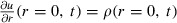

Having set the frame, we proceed to choice of parameters for the simulations. As here we deal with a generic situation, we fix the product of D and κ through the relationship (2), choosing for v the typical value, 4 mm/year for the diameter expansion (34, 35). Thus, we reduce the number of parameters and, in what follows, we vary only κ, D being determined by (2). The range of values of κ can be delimited based on results of (29), which indicate that low‐grade gliomas should have values of κ between 0.1 and 10/year.

Range of values of κ to explore is large, but we further constrain the model with a linearity condition that is related to results of (34) where linear growth was obtained for tumours of various radii, the smaller of which were around 10 mm. In the model, we therefore require that growth of radius over time be linear already at a certain radius, the value of which we fixed at 15 mm. The way to impose this constraint is by calculating the tangent of r(t) curve at r = 15 mm and require that it does not exceed half the theoretical value of diametric velocity by more than 20% (an argument supporting the choice of this value will be presented in section 4 below, dealing with real cases).

We solve eqn (5) by discretizing it over a radial mesh of size Δr = 0.002 mm with time step Δt = 0.01 yr, using an implicit scheme for diffusion and homographic‐type discretization for the logistic portion. Cell radius has been taken as around 20 μm = 10Δr. To characterize detectable parts of the tumour, we have defined tumour radius as the point where density is a given fraction of maximal, threshold ρ _* being fixed at the value 0.02, as used in (29). A typical result is shown in Fig. 1, top left. Linear growth of radius is clearly visible for large values of r. In this case, with κ = 1/year and v = 3 mm/year, relative error between slope of the tangent at r = 15 mm and half of the theoretical value of velocity, is equal to 13%.

Figure 1.

 Definition of the different times of tumour onsets used in the article. Top, left: Simulated radius of a tumour obtained from eqn (4) with κ = 1/year and v = 3 mm/year (v being the diametric velocity of expansion of the tumour) as a function of time. The continuous straight line materializes the asymptotic linear growth, while the dashed line corresponds to the tangent of the curve at the point r = 1.5 cm. The slope of the continuous straight line coincides with half the value of the diametric velocity. Bottom, left: For the same tumour, cell density at r = 0. The grey band corresponds to the invisible phase of the tumour, when the cell density is smaller than the detection threshold (materialized by the horizontal dashed line at density equal to 0.02). Top, right: Different regimes for the evolution of the radius of a tumour. The plain line (κ = 1/year, D = 2.4 × 10⁻³ mm²/year) displays an invisible phase, whereas the dashed‐dotted (κ = 1/year, D = 2.1 × 10⁻³ mm²/year) and the dashed lines (κ = 1/year, D = 10⁻³ mm²/year) correspond to always visible tumours. Bottom, right: time difference t _l − t _b between the tumour onset predicted by the linear approximation and the biological onset of the tumour predicted by the proliferation–diffusion model as a function of the threshold ρ _* (black line) and as a function of the initial radius r ₀ of the tumour (grey line) where we have added the time necessary for the tumour to reach this radius r ₀, starting from one cell and assuming a pure proliferation with the same coefficient (κ = 2/year and v = 4 mm/year).

In simulations of high‐grade gliomas, the typical initial condition is a small tumour mass (quite often, a delta function) comprising 10³–10⁴ cells. This is justified by the assumption that tumour growth begins with a simple proliferation stage and only at the end of that phase, diffusion initiates, leading to description by the diffusion–proliferation model (27, 30). However, when one is interested in total life‐time of the tumour, duration of this proliferative phase must be taken into account. As nothing is known concerning the appearance of grade II gliomas, it is easier to assume that they start from a very small tumour mass comprising of just a few cells, and consider that tumour evolution is governed from the outset by a diffusion–proliferation model. Initial radius of the small tumour mass is r ₀, in cell radius units. We generally set r ₀ = 1 (We shall come back to the question of size of the initial mass in the next section).

Computing general case time of genesis

Figure 1 top left, illustrates biological onset of tumour t = t _b = 0. At time t = t _b, the first cells begin to proliferate and migrate. But over prolonged time periods, cell density is low and stays beneath the detection threshold (Fig. 1 bottom left). Thus, there is an invisible phase where tumour expansion is slowed by competition between cell migration and proliferation, and the radius stays equal to zero for quite an appreciable amount of time. Radiologically determined tumour onset (t = t _r, Fig. 1 top left) occurs when the visible radius of the tumour begins to be larger than zero and is obviously larger than at time of the biological onset.

We see clearly that linear extrapolation backwards (t = t _l, Fig. 1 top left) cannot provide accurately either time of biological tumour onset or time radiologically predicted by the more sophisticated model. Using the proliferation‐diffusion model, due to the invisible phase, the tumour enters linear growth only at later stages, and thus linear extrapolation misses the real date of biological tumour genesis. Because of curvature of temporal evolution of tumour radius, the linear extrapolation also misses date of radiological onset of the tumour. As t _b < t _l < t _r, tumour onset given by linear approximation always underestimates biological age of the tumour at time of MRI scan, and overestimates radiological age of the tumour.

Below, we focus on measurement of time difference between date of genesis of the tumour provided by linear extrapolation and real biological starting time of tumour evolution. As, in our simulations, tumour evolution begins at time t = 0; time difference t _l − t _b can directly be read off Fig. 1, top left, as time when linear extrapolation cuts the horizontal axis.

As we have seen above, tumour growth over time depends on many parameters. It is thus of utmost importance, before attempting any application to real‐life data, to study sensitivity of the correction, t _l − t _b, to the multitude of factors that may influence its value. A factor which can be important in determination of t _l − t _b is value of threshold ρ _*, which was fixed at 0.02 for results of Fig. 1 left. In Fig. 1 bottom right, we show variation of t _l − t _b when ρ _* is allowed to vary from 0.01 to 0.1, while κ is fixed to 1.5/year (black curve). It is notable that dependence of t _l − t _b on ρ _* is not strong, the former varying by roughly 30% for an order of magnitude variation of the latter.

As explained above, our simulations up to now, were performed with an initial tumour mass of radius of one cell, r ₀ = 1 in cell radius units. However, it is interesting to examine in detail effects of variation in size of the initial tumour r ₀ on correction time t _l − t _b. The strategy we have adopted was to assume that the tumour, starting from one cell, grew by simple proliferation up to N cells (corresponding to tumour radius r ₀ with and r ₀ in cell radius units), whereupon diffusion–proliferation sets in. The main hypothesis was, in view of absence of information, to use the same proliferation coefficient κ for initial phase of pure proliferation and subsequent diffusion‐proliferation phase. Correction time was obtained by addition of proliferation time (which is equal to ) to the value of t _l − t _b obtained from simulation of (5) with initial condition of sphere of radius r ₀ and density 1. Results of variation of t _l − t _b as a function of r ₀ are shown in Fig. 1 bottom right (grey curve). These were obtained from simulation of (5) with v = 2 mm/year and κ = 2/year. We remark that variations can be quite appreciable when r ₀ varies from 1 to 100, but since nothing justifies a choice of a large initial tumour size, in applications that follow in the next section, we restrict ourselves to initial conditions corresponding to tumours of radius 1.

Clearly, parameters D and κ appearing in the model equation are also expected to play an important role in determination of value of the correction. We represent difference t _l − t _b between time of biological tumour genesis calculated with the diffusion–proliferation model and with linear extrapolation, in (D, κ) Fig. 2. There are two frontier lines between the coloured area (where constraints of linearity and maximum time evolution are satisfied) and the grey area (where at least one condition is not satisfied). The frontier at‐large diffusion coefficient is related to linearity constraint and its equation is: κ/D = 1.3/mm². Frontiers at small diffusion coefficient values are related to radius of 15 mm not being reached after maximum time of 50 years. Minimum value of velocity that allows reaching a radius of 15 mm after evolution of 50 years is 0.3 mm/year, which roughly corresponds to the equation of the second frontier. The diagram that depicts difference t _r − t _l between times of radiological tumour genesis calculated with the diffusion–proliferation model, and tumour onset estimated with linear extrapolation, in the (D, κ) diagram is very similar to diagram of t _l − t _b. Maximum is also reached for small values of κ and D, and its value is around 8 years, compared to 35 years for t _l − t _b (data not shown). We remark readily that time difference t _l − t _b on date of birth of the tumour increases when the proliferation coefficient κ decreases and can exceed 25 years for κ ≈ 0.25/year. On the other hand, when κ is equal to 10/year, t _l − t _b is close to zero. When the value of v is taken equal to 4 mm/yr (mean diametric velocity for low‐grade gliomas), variations of t _l − t _b change between 1 year for κ = 10/year and 7 years for κ = 1.2/year (at the limit of linearity).

Figure 2.

 Time difference t_l ‐ t_b between the tumour onset predicted by the linear approximation and the biological onset of the tumour predicted by the proliferation‐diffusion model, represented in colour levels, in the (D, κ) plane. The grey zone corresponds to cases that do not fulfil the constraints, i.e. either the evolution of the radius is not linear at r = 15 mm or the radius r = 15 mm is not reached after 50 years of tumour growth.

Application to cases involving patients

Having established usefulness of estimation of tumour genesis in a generic case, we now turn to applications to cases where we deal with real‐life patients. A series of 264 patients with grade II glioma is used, followed up between 1992 and 2009 in a French glioma study group [Réseau d’Etude des Gliomes (REG), France] and satisfying the following criteria (40): (i) adult patients, older than 18 years at MRI scan; (ii) absence of definite contrast enhancement on T1‐enhanced image, defined by nodules of high intensity; (iii) histological diagnosis of supratentorial hemispheric WHO grade II gliomas; and (iv) MRI follow‐up before treatment, allowing to estimate diametric velocity of expansion of the tumour (a minimum of two available scans). Patients were excluded when oncological treatment was administered (except for stereotactic biopsy) or when anaplastic transformation had occurred, either proved histologically or suspected, when a contrast enhancement appeared on MRI. For each MRI, three diameters were manually measured always by the same neurosurgeon who was blind to patient and examination data, and who did not participate in subsequent analysis of the data. In the axial plane, the largest diameters of anterior–posterior axis and perpendicular transverse axis were measured on T2‐weighted images. In the sagittal plane, only T1‐weighted image was available and was used to measure largest diameter along the vertical axis. Mean diameter was obtained as geometric mean of the three diameters, that is cube root of their product. For each patient, the curve providing velocity of expansion of mean tumour diameter as function of time was fitted by linear regression. Diametric velocity of expansion was obtained from the slope of the linear regression.

An estimate of uncertainty of value of velocity has been obtained in (41): mean tumour diameter measured as geometric mean of three diameters and, on the other hand, from volume of the tumour calculated from full 3D tumour segmentation. Difference in mean tumour diameter between the two methods is around 3 mm (i.e. 7%), leading to an error on the estimate of the diametric velocity of 0.8 mm/year (i.e. 20%).

The error on the measurement of the diameters becomes predominant when number of different scans is low and when scans are close in time. We therefore decided to exclude patients with two scans and with too short follow‐up, for which relative error in velocity was larger than 20%.

We selected patients presenting diametric velocity of expansion between 1 and 8 mm/year, since, as shown in previous publications of some of the present authors, for velocities in this range, radius evolves linearly with time (34). Moreover, as explained in (35), despite absence of histological criteria of anaplastic transformation, clinical evolution of tumours with high rate of evolution (velocities larger than 8 mm/year) is closer to that of anaplastic gliomas. To have a population as homogeneous as possible, we excluded these patients.

Distributions of ages and radii of the 144 selected patients at time of first MRI examination are represented in Fig. 3. In this distribution, and the ones that follow, we give mean values of distribution as well as corresponding standard deviation, denoted σ. We classified patients into two groups according to diametric velocity: one is 1–4 group that contains all patients with diametric velocity between 1 and 4 mm/year and the other is the 4–8 group that gathers all patients with a velocity between 4 and 8 mm/year (as we will see later, in some distributions, two peaks corresponding to these two groups do appear). In all figures, the blue histogram is distribution for all patients, the red corresponds to distributions for the 4–8 group and the green histogram corresponds to distributions for the 1–4 group. The 4–8 group contains 63 patients (age: mean = 36.1 years, σ = 11 years), 1–4 group contains 81 patients, slightly older than in the previous group (age: mean = 39.8 years, σ = 10 years).

Figure 3.

 Patients ages and tumour radii at the time of the MRI examination (clinical data). Left: Distribution of patient ages at the time of the MRI examination for all patients (blue histogram, mean = 37.4 years, σ = 10.0 years), for patients with diametric velocities between 1 and 4 mm/year (green histogram, mean = 39.8 years, σ = 11.0 years) and for patients with velocities between 4 and 8 mm/year (red histogram, mean = 36.2 years, σ = 10.0 years). Right: Distribution of tumour radii at the time of the MRI examination for all patients (blue histogram, mean = 20.9 mm, σ = 5.7 mm), for patients with velocities between 1 and 4 mm/year (green histogram, mean = 20.8 mm, σ = 5.1 mm) and for patients with velocities between 4 and 8 mm/year (red histogram, mean = 22.1 mm, σ = 6.0 mm).

We analysed data of patients using the model introduced in the previous sections, in the following way. For each patient, diffusion–proliferation equation was numerically solved for proliferation coefficients κ between 0.1 and 10/year. As the diametric velocity of tumour growth is given for each patient, one value of the proliferation coefficient κ leads to a unique value of the diffusion coefficient D and thus a unique solution for evolution of radius of the tumour as a function of time. We imposed several constraints and if one of them was not satisfied, the value of κ was rejected:

• 1 biological birthdate of the tumour, estimated with the proliferation–diffusion model, should not precede the birthdate of the patient.
• 2 required linearity for evolution of tumour radius for radius values larger than 15 mm by comparing value of the slope at 15 mm with half the theoretical value of the velocity. If value of the slope was larger than 1.2 times half the theoretical value of velocity, value of the proliferation coefficient was rejected (value of 20% variation for velocity was chosen, consistent with experimental error).
• 3 cell density should not have reached saturation more than 5 years earlier than time of first MRI examination of each patient (tumour being saturated when density at centre of the tumour exceeds 0.99). This is justified because we were dealing with grade II gliomas, characterized by absence of definite contrast enhancement on T1‐enhanced image and thus absence of angiogenesis (42). The value of 5 years is arbitrary, but this constraint was not very restrictive. Imposing this condition, we obtained acceptable values of κ up to almost 10/year. These values are already much higher than the ones proposed in (29) for grade II gliomas: in their diagram [see figure 9 in (29)], maximum value of κ is around 2/year. As explained in Model for the growth of grade II gliomas, as κ increases, minimum of the density curve occurs earlier and is shallower, thus saturation is rapidly attained. We can illustrate this in the example of a slowly growing tumour, with v = 2 mm/year. If we take a proliferation coefficient κ = 10/year, diffusion coefficient is equal to 6 × 10⁻³ mm²/year. This tumour is very compact and density at the centre reaches saturation already after t = 1.5 years, when the radius is only 1 mm. This is not compatible with what we know from grade II gliomas, which are characterized by high diffusivity and a low cell density (3).

Given these constraints, only a small range of proliferation coefficients lead to acceptable solutions for each patient; we consider that all these values of κ are equally acceptable. Each patient has uniform distribution of possible values of κ, and thus has also uniform distribution of possible D, of possible model‐obtained age of the tumour at the first MRI examination and of possible model‐obtained ages of the patient at onset of the tumour. These distributions are normalized, that is, each bin represents probability of value of the bin. This probability is used as weight for population distribution with all the patients.

As each patient is characterized by a given value of velocity, the whole range of acceptable values of κ appears as a straight line in the logarithmic diagram (D, κ). To situate clinical cases with respect to our theoretical study, we include straight lines representing acceptable values of parameters for all patients in the diagram, representing the region where correction to estimation of time of tumour genesis is acceptable, as shown in Fig. 4, left. Note that some patients did not appear as they did not have any acceptable solutions. More precisely, no patients of the 4–8 group had zero acceptable solutions in the chosen range of proliferation coefficients, whereas 24 patients of the 1–2 group did not have any acceptable (κ, D) solution.

Figure 4.

 Range of acceptable parameters of the model for each patient. Left: Superposition of the frontiers of the (D, κ) diagram of the Fig. 2 and the lines corresponding to the range of acceptable parameters D and κ for all patients. One coloured line corresponds to one patient. Right: the model‐obtained age of the tumour at the first MRI examination as a function of the diffusion coefficient for all patients. One coloured line corresponds to one patient.

We also calculated distributions for the patient population, from normalized distributions for each patient. Let us focus on distribution of model‐obtained ages of tumours at first MRI examination. In Fig. 4, right, the diagram represents range of acceptable tumour ages at time of MRI for each patient, as a function of D. Let us take the example of a patient having an acceptable tumour age at time of MRI between 21 and 29 years. A tumour age bin is chosen, here equal to 2 years. The chosen patient will have a non‐zero contribution to 5 bins, so probability of each of these bins is equal to 0.2. Thus, contribution of this patient to each of these 5 bins is value of the probability of this time value, here 0.2. In the other bins, his contribution is zero. To build the population distribution, in each tumour age bin between 0 and 50 years, contributions of all patients are added. Therefore, sum of the contents of all bins is equal to number of patients, for all population distributions presented in the following.

Population distribution of tumour ages is presented in Fig. 5, right. There are two peaks in distribution of model‐obtained age of the tumour at first MRI examination, peaks being associated with the two different groups of patients that we have distinguished on the basis of values of velocity. Green distribution corresponds to patients with a velocity between 1 and 4 mm/year (mean = 24.8 years, σ = 9.0 years), and red distribution to patients with a velocity between 4 and 8 mm/year (mean = 11.5 years, σ = 3.7 years).

Figure 5.

 Calculated age of the patients at tumor onset and of the tumor at the time of the MRI examination. Left: Distribution of model‐obtained age of the patient at the onset of the tumour for all patients (blue histogram, mean = 18.1 years, σ = 9.6 years), for patients with velocities between 1 and 4 mm/year (green histogram, mean = 14.9 years, σ = 9.9 years) and for patients with velocities between 4 and 8 mm/year (red histogram, mean = 24.7 years, σ = 9.4 years). Right: Distributions of model‐obtained age of tumour at the time of MRI examination of all patients (blue histogram, mean = 17.6 years, σ = 9.6 years), for patients with velocities between 1 and 4 mm/year (green histogram, mean = 24.8 years, σ = 9.8 years) and for patients with velocities between 4 and 8 mm/year (red histogram, mean = 11.5 years, σ = 3.7 years).

Distribution of patient ages at onset of the tumour is represented in Fig. 5, left. This distribution also exhibits two peaks corresponding to the two groups of velocities [for the 4–8 group distribution (red), mean = 24.7 years, σ = 9.4 years, for the 1–4 group distribution (green), mean = 14.9 years, σ = 9.9 years]. Distribution of values of the proliferation coefficient κ (mean = 2.8/year, σ = 2.2/year, maximum of distribution corresponding to value κ = 1/year) possible for patients is presented in Fig. 6 top, right. Corresponding distribution of values of the diffusion coefficient is shown in Fig. 6 top, left (mean = 0.6 mm²/year, σ = 0.3 mm²/year, maximum distribution corresponds to value D = 0.55 mm²/year).

Figure 6.

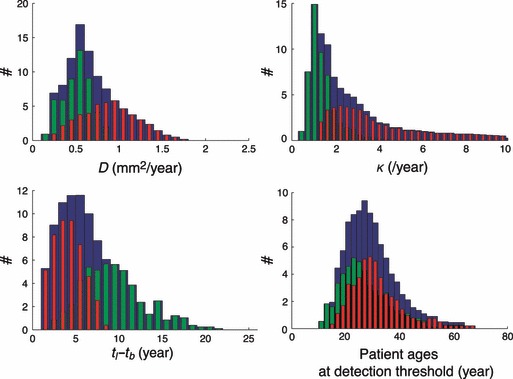
 Acceptable parameters of the model and calculated time difference and patient age at detection threshold. Top, left: Distribution of values of D for all patients (blue histogram, mean = 0.6 mm²/year, σ = 0.3 mm²/year), for patients with velocities between 1 and 4 mm/year (green histogram, mean = 0.4 mm²/year, σ = 0.1 mm²/year) and for patients with velocities between 4 and 8 mm/year (red histogram, mean = 0.8 mm²/year, σ = 0.3 mm²/year). Top, right: Distribution of values of κ for all patients (blue histogram, mean = 2.7/year, σ = 2.2/year), for patients with velocities between 1 and 4 mm/year (green histogram, mean = 1.3/year, σ = 0.7/year) and for patients with velocities between 4 and 8 mm/year (red histogram, mean = 3.9/year, σ = 2.2/year). Bottom left: distribution of the time difference t _l − t _b between the tumour onset predicted by the linear approximation and the biological onset of the tumour predicted by the proliferation–diffusion model for all patients (blue histogram, mean = 6.1 years, σ = 3.8 years), for patients with velocities between 1 and 4 mm/year (green histogram, mean = 8.9 years, σ = 3.6 years) and for patients with velocities between 4 and 8 mm/year (red histogram, mean = 3.7 years, σ = 1.6 years). Bottom right: Distribution of patient ages at the time of detection of the tumour for all patients (blue histogram, mean = 28.4 years, σ = 9.5 years), for patients with velocities between 1 and 4 mm/year (green histogram, mean = 26.4 years, σ = 9.3 years) and for patients with velocities between 4 and 8 mm/year (red histogram, mean = 30.0 years, σ: 9.0 years).

In Fig. 6, bottom right, age of patients when tumours become detectable (1–4 group: mean = 26.4 years, σ = 9.3 years; 4–8 group: mean = 30.0 years, σ = 9.0 years), that is, when density at the centre of the tumour crosses the detection threshold. For 1–4 group, the invisible phase of tumour growth lasts 13 years (mean = 13.2 years, σ = 5.5 years) and after this invisible period, the tumour still grows for 11.5 years (mean = 11.5 years, σ = 4.2 years) before triggering clinical symptoms. For the 4–8 group, the invisible phase lasts 5 years (mean = 5.4 years, σ = 2.4 years) and after the invisible period, the tumour still grows for 6 years (mean = 6.1 years, σ = 2.0 years) before triggering clinical symptoms.

Time difference t _l − t _b between tumour onset predicted by the linear approximation and biological onset of the tumour predicted by the proliferation‐diffusion model, is presented in Fig. 6, bottom left (1–4 group: mean = 8.9 years, σ = 3.6 years; 4–8 group: mean = 3.7 years, σ = 1.6 years). As explained in the section above devoted to a general case, backwards linear extrapolation always underestimates tumour age. We find here that a correction depending on diametric velocity should be added to the estimation of tumour age obtained by linear extrapolation.

To make dependence of the different variables on velocity more precise, patients have been divided into five small groups according to velocity of their tumour growth. The first group has patients with velocities between 1 and 3 mm/year, the second between 3 and 4.5 mm/year, the third between 4.5 and 6 mm/year, and the fourth between 6 and 8 mm/year. A fifth group (with velocities between 8 and 20 mm/year) has also been considered here. Each of these groups has each more than 30 members. Means of distributions of patient ages at onset of the tumour, of tumour age at time of first MRI examination and of the time difference t _l − t _b between tumour onset predicted by linear approximation and biological onset of the tumour predicted by the proliferation‐diffusion model, versus mean diametric velocity of each group, are given in Fig. 7. Tumours tend to occur later in life of patients, as velocity increases (curve with plain circles) and is also detected earlier in its evolution (curve with stars), and linear approximation provides a more and more accurate estimation of the date of genesis of the tumour (curve with diamonds). Velocities larger than 8 mm/year) appear here as a dashed line as linear growth of diameter of tumours has not been shown for velocities larger than 8 mm/year. However, we decided to add this high velocities group, as it follows the same tendency as that of the others, see Fig. 7.

Figure 7.

 Evolution of the mean calculated tumor age at time of MRI examination, patient age at the tumour onset and time difference as a function of the growth velocity of the tumour. In this figure, patients have been divided into five small groups according to their velocity. The first group contains patients with velocities between 1 and 3 mm/year, the second between 3 and 4.5 mm/year, the third between 4.5 and 6 mm/year, the fourth between 6 and 8 mm/year. A fifth group with velocities between 8 and 20 mm/year has been considered only for this figure, as it follows the same tendency as the others. The evolution of the means of population distributions are depicted here. Evolution of the mean tumour age at the time of the MRI examination (stars), of the mean patient age at the onset of the tumour (plain circles), of the mean time difference t _l − t _b between the tumour onset predicted by the linear approximation and the biological onset of the tumour predicted by the proliferation–diffusion model (diamonds), as a function of the growth velocity of the tumour v. The error bars represent the standard deviations. The curve of t _l − t _b as a function of the velocity v can be roughly fitted by the function 20/v (year), with v expressed in mm/year (grey line) (it is not the better fit, but we preferred a simple formula).

Tumours discovered incidentally

Usually, gliomas are discovered during an MRI examination when a patient presents with symptoms such as seizures. However and rarely, some gliomas are incidentally discovered during an MRI examination for a different condition. Patients are still asymptomatic and mean radius of tumours is smaller than in patients with symptoms. We therefore expect tumour age at time of first MRI examination to be smaller. Incidental tumours used here have already been described in (37). Of the 47 patients cited in that investigation, 22 were found to be eligible according to the constraints used for symptomatic patients.

As in the case of symptomatic patients, asymptomatic ones were also divided into two groups according to velocities of expansion. Distribution for asymptomatic patients with tumour velocities larger than 4 mm/year is presented in Fig. 8, left, red histogram (number of patients: 13; mean = 7.8 years, σ = 3.3 years). The mean of this distribution was smaller by roughly 3 years compared to mean of the corresponding distribution for patients with symptoms (4–8 group, mean distribution of tumour ages at time of first MRI examination: 11.5 years, σ = 3.7 years). Due to the low number of patients (9), distribution of tumour ages at time of first MRI examination for asymptomatic patients with velocity smaller than 4 mm/year (green histogram) is very large, almost flat, and is far from Gaussian distribution; mean of the distribution is thus, not informative.

Figure 8.

 Distributions for asymptomatic patients. Left: Distribution of tumour ages at time of the first MRI examination (calculated with the model) for all asymptomatic patients (blue histogram, the mean is not representative), for patients with velocities between 1 and 4 mm/year (green histogram, the mean is also not representative) and for patients with velocities between 4 and 8 mm/year (red histogram, mean = 7.8 years, σ = 3.3 years). Right: Radius of the tumour versus the age of the patient studied in (38) with two different proliferation coefficients κ = 1.5/year (thin line) and κ = 5.7/year (thick line). The biological onsets of the tumour in each case t _b1 and t _b2 are indicated by small vertical bars. t _MRI1 and t _MRI2 (dashed arrows) indicate the two MRI examinations that the patient underwent.

An interesting test is the case of the patient described in (38). A young man, born in 1978, was clinically followed up over 15 years after surgery in 1995, when he was 17, due to malformation of his cerebellum. During this period, he underwent whole brain MRI examination in 1997, which did not reveal any tumour. However, in 2009, a new whole brain tumour MRI examination revealed a grade II glioma in the supra‐tentorial region. Radius of the tumour was measured (r = 14.5 mm) and its diametric growth velocity was estimated (v =4 mm/year).

We simulated the evolution of this tumour, with two quite different values of proliferation coefficient, κ = 1.5/year (thin line in Fig. 8, right) and κ = 5.7/year (thick line in Fig. 8, right) over the patient’s life (horizontal axis represents age of the patient), but with same value of velocity (so for long time periods, the two curves are parallel). These two values are in the range of acceptable values of κ for this patient, given the constraints described previously (age, linearity, saturation). Vertical arrows indicate dates of whole brain MRI examination, in 1997 and 2009. In the case where κ = 1.5/year, the tumour started when the patient was 18. Linear approximation that would lead to onset of the tumour when the patient was 24 underestimates presence of the tumour by 6 years. It is interesting to remark that the 1997 MRI examination occurred during the invisible phase of this tumour. In the case where κ = 5.7/year, the tumour began when the patient was almost 23 and time difference t _l − t _b between tumour onset predicted by linear approximation and biological onset of the tumour predicted by the proliferation–diffusion model, is only 1 year. In this case, MRI examination had occurred before onset of the tumour. In conclusion, the model is consistent with what has been observed clinically.

Discussion and outlook

In this article, we have set out to estimate date of birth of grade II gliomas based on clinical observations analysed using a macroscopic model. This enterprise is justified by the fact that evolution of grade II gliomas (at least as long as the gliomas do not evolve into high‐grade ones) presents regular behaviour, which lends itself to quantitative estimation. Thus, in previous studies by some of the present authors, it has been shown that mean diameter of a grade II tumour expands linearly over time. Moreover, diametric velocity of an iso‐density curve of such a tumour could be estimated and the value turned out to be around 4 mm/year (34, 35). Linearity of growth of tumours diameter suggested a simple approach to estimating tumour genesis: assumption that growth is linear (and with the same velocity) from the outset and extrapolate backwards from measured radius back to the moment when the radius was zero. However, this approach is too simplified, there is no reason whatsoever that such a tumour would enter the linear‐growth phase from the outset, and there are no experimental data to support this assumption. All cases studied where linearity was obtained, corresponded to a radius of a rather well‐established tumour, typically larger than 1 cm (34). Thus, we decided to consider a slightly more sophisticated description, based on a diffusion–proliferation model, for explanation of properties of the tumour. The advantage of such a model is that it leads to linear growth of the tumour radius, albeit asymptotically. Thus, one would expect a difference t _l − t _b between results for tumour genesis obtained from simple reverse extrapolation and the diffusion–proliferation model.

Our first step, before using a diffusion‐proliferation model to analyse clinical data, was to establish its validity and sensitivity of results with respect to the various parameters and assumptions. The first question was whether one could always obtain an acceptable answer, corresponding to positive correction to the simple backward extrapolation. As linear behaviour appears only asymptotically, this is not a priori guaranteed. However, over a very large range the various parameters of the model (and in particular those that are interesting, given our data), this is indeed the case. The next question concerns the role played by the various parameters of the model. The first step was to investigate this question without reference to specific patients. As expected, difference t _l − t _b between the diffusion‐proliferation model and simple reverse extrapolation, for the date of tumour birth depends crucially on diffusion and proliferation coefficients, the two being linked by the above relationship. On the other hand, variation in detection threshold over an order of magnitude led to a very small variation in t _l − t _b. A crucial assumption of our model was that of tumours starting essentially from only one tumour cell. The results depend on this assumption, but in the light of absence of any contradictory evidence, we feel that this assumption is more natural than any arbitrary choice of initial radius. In the second section, we explained how the linearity constraint was implemented: at fixed tumour radius, 15 mm here, we require that local slope of the r(t) curve does not differ from the asymptotic half value of diametric velocity, by more than 20%, discarding parameters that did not satisfy this constraint. Moreover, given that application of the model targets human patients, we introduced a further constraint, namely that linearity be reached before a time‐lapse of 50 years, a conservative constraint. Finally, with reference to clinical data, in particular absence of observed angiogenesis in the low‐grade gliomas under study (42), we introduced a further constraint in the model related to saturation. More precisely, we required the centre of the tumour to have reached saturation density over less than 5 years. Thus, we require that saturation at the core of the tumour should be recent.

Once the model was shown to give reasonable results in a generic case, we proceeded to apply it to the analysis of data on real‐life patients. The main difference with respect to the generic case is that for every patient, we have a fixed value of the diametric velocity of tumour growth, as well as the value of the tumour radius, and the age of the patient at the moment of the first MRI examination. We thus reject here the values of the parameters when the model‐obtained age of the tumour at the first MRI examination is larger than the age of the patient. We discuss now our main results:

Individual information

The model does not provide a unique solution for each patient as several values of κ are acceptable, leading to several possible model‐obtained ages of the tumour at first MRI examination, and also several possible model‐obtained ages for the patient at onset of the tumour (all of values being equally probable). However, for patients whose distributions are not too large, this approach could be useful. It could be interesting, for example, to compare distributions of proliferation coefficient and diffusion coefficient with values obtained by other methods (29). We applied individual analysis to the case of an asymptomatic patient, and successfully showed that range of model‐obtained ages of the tumour at first MRI examination were consistent with radiological follow‐up of the patient. Early MRI examination did not reveal any tumour and our model predicts that at this moment, the tumour did not yet exist, or was in its invisible phase.

Contrary to the model, linear approximation yields a unique age for the tumour at first MRI examination (and therefore, a unique age for the patient at tumour onset). However, this value is always underestimated. We showed that mean correction (obtained from population analysis) that had to be added to age of the tumour at first MRI scan, given by linear approximation depends on velocity v, see Fig. 7. Curve of the correction as a function of diametric velocity of Fig. 7 can be roughly approximated by function 20/v (year) with v in mm/year. Thus, if one required to estimate age of the tumour at time of MRI, one could add (roughly) 20/v to the age provided by the linear approximation, that is, age of the tumour is roughly (20 + d _MRI)/v (with d _MRI being diameter of the tumour at first MRI scan, expressed in mm). This result is new evidence that measurement of diametric velocity of expansion of a tumour is a very important and useful parameter.

A further interesting result is that we have shown that within range of velocities smaller than 8 mm/year, and with the hypothesis that the initial tumour mass is composed of only one cell, we are always in the regime where an initial invisible phase exists. This would not always be the case with larger value of r ₀, for example. This hypothesis is consistent with what is known of the biology of grade II gliomas, especially that cell density remains low even at the centre of the tumour.

Population information

Uniform distributions of tumour age, proliferation coefficient and diffusion coefficient for each patient were combined, leading to distributions for the patient population. Mean proliferation coefficient is 2.8/year (σ = 2.2/year, maximum of the distribution, that is, the most probable value, corresponds to value κ = 1/year) and mean diffusion coefficient is 0.6 mm²/year (σ = 0.3 mm²/year, the most probable value being D = 0.55 mm²/year).

Some of these distributions are bimodal (age of patients at onset of the tumour and model‐based age of the tumour at time of MRI), corresponding to two groups of velocities. We thus defined two groups of patients: those with diametric velocities between 1 and 4 mm/year (the 1–4 group), and those with diametric velocities between 4 and 8 mm/year (the 4–8 group). That we can distinguish several peaks in distribution of ages of tumours at the moment of first MRI examination will have to be confirmed by new studies, with more patients and more precise measurement of velocities. The two peaks arise because age of a tumour is close to r/v, that mean radius of the 4–8 group is slightly lower than mean radius of the 1–4 group (cf Fig. 3 right), and that 1/v is also lower for the 4–8 group than for the 1–4 group. These bimodal distributions could suggest the existence of two different types of tumour, slowly growing tumours (v between 4 and 8 mm/year) and very slowly growing ones (v between 1 and 4 mm/year).

Tumours with the highest velocities are easy to accommodate within our model: all patients have at least one solution for κ in the 0.1–10/year range and most of them have many solutions, leading to large distribution of values of κ. Analysis of age of patients at onset of the tumour leads to a moderately large distribution with a peak at around 25 years, for the 4–8 group. Distribution of age of the tumour at the moment of first MRI examination is quite narrow, leading to a typical value of 11 years, with an invisible phase of around 6 years. Mean correction that has to be added to linear approximation of age of the tumour at time of MRI is equal to 3.7 years.

Contrary to the 4–8 group, some patients in the 1–4 group do not have any solution for κ in the 0.1–10/year range. This means that the model cannot describe correctly all of these very slowly growing tumours. As these tumours develop over a long time period (mean tumour age at moment of first MRI examination is around 25 years, with 13 years of invisible phase), it is possible that proliferation coefficient and diffusion coefficient underwent changes during the tumours’ evolution. If such change happened during the invisible growth phase, it could explain why no change in evident slopes have been observed. Moreover, these slow growing tumours occur during adolescence. If v is between 1 and 4 mm/yr, mean age for outbreak of such a tumour is around 15 years of age. At that moment, many hormonal changes occur, which might explain changes also in characteristics of tumours. In this group, patients are younger when the tumour begins, but at time of diagnosis, the tumour is older, and mean correction that must be added to estimate of linear approximation is larger than in the 4–8 group (around 8.9 years compared to 3.7 years). It would be interesting to investigate whether these two types of tumour, defined here on criteria of diametric expansion velocity, correspond to biologically different tumours that could have different prognoses or could respond to different types of treatment. These two types of tumour become detectable at mean patient age of 30 years, within the approximation of the model; if confirmed, this result could potentially have clinical applications, for example, in formulating strategies for early tumour detection. A further result was obtained when admissible values of diffusion and proliferation coefficients for all patients were plotted on a κ–D diagram. There, the region of grade II gliomas was represented as a zone that is off‐centred compared to figure 9 of (29), associated with slightly larger values of κ (mean = 2.7/year, σ = 2.2/year) and, naturally, smaller values of D (mean = 0.6 mm²/year, σ = 0.3 mm²/year) than in (29). More precisely, we found that the zone where tumour radius evolution is linear at radius r = 15 mm, is defined by κ/D > 1.3/mm².

We also confronted the model with incidental tumours. As these have been discovered fortuitously, one would expect that age of tumours at time of the first MRI examination be lower than age of tumours in the case of symptomatic tumours. Our model indeed predicts distribution of tumour ages peaked at lower values, the shift being of the orders of 3 years, for the 2–4 group. This value of shift is in agreement with clinical data; clinical symptoms occur at mean interval of 55 months after radiological incidental discovery (37).

All these results have of course to be taken with a grain of salt as several strong assumptions have been made: we consider that tumours have a spherical geometry; we do not take into account either the anisotropy of the brain or influence of skull or other natural obstacles (13), nor difference between gray and white matter (12). Still, as mean diameter of the tumours does increase linearly, we can reasonably assume that influence of geometry is not very important. Many biological processes are also neglected (for example, metabolism of cells involved); we believe that during the linear growth period, the two biological processes that dominate are diffusion and proliferation of cells. While our model provides a satisfactory description of genesis and growth of low‐grade gliomas, it does not allow for predictions on the appearance of malignancy that occur ineluctably for these tumours, manifested by substantial increase in diametric velocity of tumour growth. As contrast enhancement regions are often nodular, we believe such a phenomenon to be associated mainly with local changes in basic parameters of the tumour (40). In particular, we will have to take into account angiogenesis in our model; this is the process by which new blood vessels are formed within the tumour, to provide additional nutrients to it; to do so, models described in (43) and (44) will constitute good starting points.

Various regimes

In this section, we have presented some analytical results obtained from the diffusion–proliferation model (neglecting saturation as an explicit solution exists only in this case) to explain different regimes of evolution of tumour radius, see Fig. 1, top right.

Green’s function of eqn (3) without saturation is

(A1)

and thus, solution of (1), with spherical symmetry, constant D, and taking δ‐function containing N ₀ cells as an initial condition. This is just

(A2)

We have introduced maximum cell concentration C _m, parameterize it in terms of auxiliary variable t ₀,

(A3)

And have used it to define cell density ρ = C/C _m.

Our initial condition for integration of (5) is a density profile equal to 1 inside a small sphere of radius r ₀ and 0 outside. However, convolution of such a density with Green’s function (eqn A1) leads to, still analytical, but rather complicated, results and thus we have preferred to use an initial condition, which is a Gaussian. We have adjusted the parameters so as to make volume of the latter equal to that of the sphere of radius r ₀ and found

(A4)

where the auxiliary parameter t ₀ is related to r ₀ by . By convoluting ρ ₀ with , we obtained the solution of the diffusion equation without saturation:

(A5)

Using this solution, it is straightforward to derive position of an iso‐density curve, characterized by value ρ _* of the density. We found

(A6)

The function r(ρ _*, t) displays an invisible phase, when the function is negative [in (23), this phase is called ‘establishment phase’]. During the invisible phase, the tumour is growing, but remains beneath the detection threshold and thus it is not visible [We have materialized the invisible phase in our Fig. 1 (left top and bottom) by a grey band]. Due to this invisible phase, linear approximation will always underestimate the age of the tumour.

Two conditions are necessary for appearance of this invisible phase. First, minimum of f(t) must occur for a positive value of t. A direct calculation yields time of minimum

(A7)

and thus the positivity condition is just

(A8)

Second, value of f(t) at its minimum must be negative, leading to the condition

(A9)

For range of parameters used here, 0.1 < κ < 10/year, 1 < v < 8 mm/year (v being the diametric velocity), and for r ₀ = 0.02 mm (we start with one cell), it is clear that the first condition for existence of an invisible phase, , is always satisfied. Of course for very small values of v and large values of κ (resulting in very small values of D), it is possible to find a regime where the invisible phase disappears. However, as we will see in the case of real‐life patients, these extreme parameters are not acceptable as they lead to very early saturation. Also, if the initial sphere radius gets larger by containing more cells, evolution of the tumour rapidly switches to the regime where there is no longer an invisible phase; density at the centre never falls below the detection threshold. The tumour would always be visible in this case. In the case of the full model with saturation, threshold between ‘with‐invisible‐phase’ regime and ‘always‐visible’ regime can no longer be calculated analytically. However, as saturation has a non‐negligible influence only in regions where density is large with respect to ρ _* (that is, at the rear of the invasion front), it negligibly affects the frontier between visible and invisible regions of the tumour. Transition between the two regimes occurs at a value of κt ₀ very close to the value obtained from the model without saturation.

Figure 1 top right shows three different regimes: the full line displays an invisible phase, whereas the other two curves correspond to always visible tumours. Evolution of the radius can have extrema (as in the case of the dashed‐dotted line) or not (as in the case of the dashed line). Any initial bump is in radius smaller than 0.1 mm and therefore it is well below resolution of MRI examination. This bump comes from the fact that at very short times, diffusion process dominates, and density at r = 0 decreases very rapidly. However, slowly, the proliferation process becomes competitive and thus density decrease stabilizes, value of density reaching its minimum and begins to increase up to maximum value of 1, see Fig. 1, bottom left.

At r = 0, the time to reach a given value of ρ = ρ _*, satisfies:

(A10)

With our parameters, t ₀ << 1 year, so we always have t >> t ₀. In this case, time to reach value ρ = ρ _* at r = 0 is given by the condition:

(A11)

As t ₀ only depends on r ₀ and D, time to reach a given value of ρ _* at r = 0 (that is, for peculiar value of ρ _* = 0.02, duration of invisible phase) decreases when κ increases and increases when D increases. In the case of the full model, with saturation, the same behaviour is observed, so as κ increases (decreases) or D decreases (increases), the invisible phase of the tumour is shorter (longer). Even for value ρ _* = 0.99 (that defines the threshold for saturation), we observed that time to reach saturation behaves in the same way, that is, the tumour saturates earlier (latter), as we would have expected intuitively.

References

- 1. Louis DN, Ohgaki H, Wiestler OD, Cavenee WK, Burger PC, Jouvet A et al. (2007) The 2007 WHO classification of tumours of the central nervous system. Acta Neuropathol. 114, 97–109. [DOI] [PMC free article] [PubMed] [Google Scholar]
- 2. Kelly PJ, Daumas‐Duport C, Kispert DB, Kall BA, Scheithauer W, Illig J (1987) Imaging‐based stereotaxic serial biopsies in untreated intracranial glial neaplasms. J. Neurosurg. 66, 865–874. [DOI] [PubMed] [Google Scholar]
- 3. Pallud J, Varlet P, Devaux B, Geha S, Badoual M, Deroulers C et al. (2010) Diffuse low‐grade oligodendrogliomas extend beyond MRI‐defined abnormalities. Neurology 74, 1724–1731. [DOI] [PubMed] [Google Scholar]
- 4. Keles GE, Lamborn KR, Berger MS (2001) Low‐grade hemispheric gliomas in adults: a critical review of extent of resection as a factor influencing outcome. J. Neurosurg. 95, 735–745. [DOI] [PubMed] [Google Scholar]
- 5. Salgaller ML, Liau LM (2006) Current status of clinical trials for glioblastoma. Rev. Recent Clin. Trials 3, 265–281. [DOI] [PubMed] [Google Scholar]
- 6. Sanai N, Berger MS (2008) Glioma extent of resection and its impact on patient outcome. Neurosurgery 4, 753–764. [DOI] [PubMed] [Google Scholar]
- 7. Mandonnet E, Pallud J, Fontaine D, Taillandier L, Bauchet L, Peruzzi P et al. (2009) Inter‐ and intrapatients comparison of WHO grade II glioma kinetics before and after surgical resection. Neurosurg. Rev. 33, 91–96. [DOI] [PubMed] [Google Scholar]
- 8. Ricard D, Kaloshi G, Amiel‐Benouaich A, Lejeune J, Marie Y, Mandonnet E et al. (2007) Dynamic history of low‐grade gliomas before and after temozolomide treatment. Ann. Neurol. 61, 484–490. [DOI] [PubMed] [Google Scholar]
- 9. Prabhu VC, Khaldi A, Barton KP, Melian E, Schneck MJ, Primeau MJ et al. (2010) Management of diffuse low‐grade cerebral gliomas. Neurol. Clin. 28, 1037–1059. [DOI] [PubMed] [Google Scholar]
- 10. Peyre M, Cartalat‐Carel S, Meyronet D, Ricard D, Jouvet A, Pallud J et al. (2010) Prolonged response without prolonged chemotherapy: a lesson from PCV chemotherapy in low‐grade gliomas. Neuro Oncol. 12, 1078–1082. [DOI] [PMC free article] [PubMed] [Google Scholar]
- 11. Giese A, Bjerkvig R, Berens ME, Westphal M (2003) Cost of migration: invasion of malignant gliomas and implications for treatment. J. Clin. Oncol. 21, 1624–1636. [DOI] [PubMed] [Google Scholar]
- 12. Swanson KR, Alvord EC, Murray JD (2000) A quantitative model for differential motility of gliomas in grey and white matter. Cell Prolif. 33, 317–329. [DOI] [PMC free article] [PubMed] [Google Scholar]
- 13. Jbabdi S, Mandonnet E, Duffau H, Capelle L, Swanson KR, Pelegrini‐Issac M et al. (2005) Simulation of anisotropic growth of low‐grade gliomas using diffusion tensor imaging. Magn. Reson. Med. 54, 616–624. [DOI] [PubMed] [Google Scholar]
- 14. Frieboes HB, Zheng X, Sun CH, Tromberg B, Gatenby R, Cristini V (2006) An integrated computational/experimental model of tumor invasion. Cancer Res. 66, 1597–1604. [DOI] [PubMed] [Google Scholar]
- 15. Guiot C, Pugnot N, Delsanto PP, Deisboeck TS (2007) Physical aspects of cancer invasion. Phys. Biol. 4, 1–6. [DOI] [PubMed] [Google Scholar]
- 16. Stein AM, Demuth T, Mobley D, Berens M, Sander LM (2007) A mathematical model of glioblastoma tumor spheroid invasion in a three‐dimensional in vitro experiment. Rep. Prog. Phys. 72, 356–365. [DOI] [PMC free article] [PubMed] [Google Scholar]
- 17. Gerisch A, Chaplain MA (2008) Mathematical modelling of cancer cell invasion of tissue: local and non‐local models and the effect of adhesion. J. Theor. Biol. 250, 684–704. [DOI] [PubMed] [Google Scholar]
- 18. Aubert M, Badoual M, Féreol S, Christov C, Grammaticos B (2006) A cellular automaton model for the migration of glioma cells. Phys. Biol. 3, 93–100. [DOI] [PubMed] [Google Scholar]
- 19. Aubert M, Badoual M, Christov C, Grammaticos B (2008) A model for glioma cell migration on collagen and astrocytes. J. R. Soc. Interface 5, 75–83. [DOI] [PMC free article] [PubMed] [Google Scholar]
- 20. Deroulers C, Aubert M, Badoual M, Grammaticos B (2009) Modeling tumor cell migration: from microscopic to macroscopic models. Phys. Rev. E 79, 031917‐1–031917‐14. [DOI] [PubMed] [Google Scholar]
- 21. Badoual M, Deroulers C, Aubert M, Grammaticos B (2010) Modelling intercellular communication and its effect on tumour invasion. Phys. Biol. 7, 046013. [DOI] [PubMed] [Google Scholar]
- 22. Tanaka ML, Debinski W, Puri IK (2009) Hybrid mathematical model of glioma progression. Cell Prolif. 42, 637–646. [DOI] [PMC free article] [PubMed] [Google Scholar]
- 23. Murray JD (2002) Mathematical Biology. II: Spatial Models and Biomedical Applications, 3rd edn Berlin: Springer‐Verlag. [Google Scholar]
- 24. Tracqui P, Cruywagen GC, Woodward DE, Bartoo GT, Murray JD, Alvord EC (1995) A mathematical model of glioma growth: the effect of chemotherapy on spatio‐temporal growth. Cell Prolif. 28, 17–31. [DOI] [PubMed] [Google Scholar]
- 25. Cruywagen GC, Woodward DE, Tracqui P, Bartoo GT, Murray JD, Alvord EC (1995) The modelling of diffusive tumours. J. Biol. Syst. 3, 937–945. [Google Scholar]
- 26. Cook J, Woodward DE, Tracqui P, Cruywagen GC, Murray JD, Bartoo GT et al. (1995) Resection of gliomas and life expectancy. J. Neurooncol. 24, 131. [Google Scholar]
- 27. Burgess PK, Kulesa PM, Murray JD, Alvord EC (1997) The interaction of growth rates and diffusion coefficients in a three‐dimensional mathematical model of gliomas. J. Neuropathol. Exp. Neurol. 56, 704. [PubMed] [Google Scholar]
- 28. Bondiau PY, Clatz O, Sermesant M, Marcy PY, Delinguette H, Frenay M et al. (2008) Biocomputing: numerical simulation of glioblastoma growth using diffusion tensor imaging. Phys. Med. Biol. 53, 879–893. [DOI] [PubMed] [Google Scholar]
- 29. Harpold HL, Alvord EC Jr, Swanson KR (2007) The evolution of mathematical modeling of glioma proliferation and invasion. J. Neuropathol. Exp. Neurol. 1, 1–9. [DOI] [PubMed] [Google Scholar]
- 30. Woodward DE, Cook J, Tracqui P, Cruywagen GC, Murray JD, Alvord EC (1996) A mathematical model of glioma growth: the effect of extent of surgical resection. Cell Prolif. 29, 269–288. [DOI] [PubMed] [Google Scholar]
- 31. Swanson KR, Bridge C, Murray JD, Alvord EC Jr (2004) Virtual and real brain tumors: using mathematical modeling to quantify glioma growth and invasion. J. Neurol. Sci. 216, 289–296. [DOI] [PubMed] [Google Scholar]
- 32. Powathil G, Kohandel M, Sivaloganathan S, Oza A, Milosevic M (2007) Mathematical modeling of brain tumors: effects of radiotherapy and chemotherapy. Phys. Med. Biol. 52, 3291–3306. [DOI] [PubMed] [Google Scholar]
- 33. Rockne R, Rockhill JK, Mrugala M, Spence AM, Kalet I, Hendrickson K et al. (2010) Predicting the efficacy of radiotherapy in individual glioblastoma patients in vivo: a mathematical modelling approach. Phys. Med. Biol. 55, 3271–3285. [DOI] [PMC free article] [PubMed] [Google Scholar]
- 34. Mandonnet E, Delattre JY, Tanguy ML, Swanson KR, Carpentier AF, Duffau H et al. (2003) Continuous growth of mean tumor diameter in a subset of grade II gliomas. Ann. Neurol. 53, 524–528. [DOI] [PubMed] [Google Scholar]
- 35. Pallud J, Mandonnet E, Duffau H, Kujas M, Guillevin R, Galanaud D et al. (2006) Prognostic value of initial magnetic resonance imaging growth rates for world health organization grade II gliomas. Ann. Neurol. 60, 380–383. [DOI] [PubMed] [Google Scholar]
- 36. Hlaihel C, Guilloton L, Guyotat J, Streichenberger N, Honnorat J, Cotton F (2010) Predictive value of multimodality MRI using conventional, perfusion, and spectroscopy MR in anaplastic transformation of low‐grade oligodendrogliomas. J. Neurooncol. 97, 73–80. [DOI] [PubMed] [Google Scholar]
- 37. Pallud J, Fontaine D, Duffau H, Mandonnet E, Sanai N, Taillandier L et al. (2010) Natural history of incidental WHO grade II gliomas. Ann. Neurol. 68, 727–733. [DOI] [PubMed] [Google Scholar]
- 38. Duffau H, Pallud J, Mandonnet E (2011) Evidence for the genesis of WHO grade II glioma in an asymptomatic young adult using repeated MRIs. Acta Neurochir. 153, 473–477. [DOI] [PubMed] [Google Scholar]
- 39. Murray JD (2002) Mathematical Biology: I. An Introduction, 3rd edn Berlin: Springer‐Verlag. [Google Scholar]
- 40. Pallud J, Capelle L, Taillandier L, Fontaine D, Mandonnet E, Guillevin R et al. (2009) Prognostic significance of imaging contrast enhancement for WHO grade II gliomas. Neuro-oncology 11, 176–182. [DOI] [PMC free article] [PubMed] [Google Scholar]
- 41. Mandonnet E, Pallud J, Clatz O, Taillandier L, Konukoglu E, Duffau H et al. (2008) Computational modeling of the who grade II glioma dynamics: principles and applications to management paradigm. Neurosurg. Rev. 31, 263–269. [DOI] [PubMed] [Google Scholar]
- 42. Daumas‐Duport C, Varlet P, Tucker ML, Beuvon F, Cervera P, Chodkiewicz JP (1997) Oligodendrogliomas. part i: Patterns of growth, histological diagnosis, clinical and imaging correlations: a study of 153 cases. J. Neurooncol. 34, 37–59. [DOI] [PubMed] [Google Scholar]
- 43. Anderson AR, Chaplain MA (1998) Continuous and discrete mathematical models of tumor‐induced angiogenesis. Bull. Math. Biol. 60, 857–899. [DOI] [PubMed] [Google Scholar]
- 44. Cooper MD, Tanaka ML, Puri IK (2010) Coupled mathematical model of tumorigenesis and angiogenesis in vascular tumours. Cell Prolif. 43, 542–552. [DOI] [PMC free article] [PubMed] [Google Scholar]