

Abstract
Motivation
Many high-throughput methods produce sets of genomic regions as one of their main outputs. Scientists often use genomic colocalization analysis to interpret such region sets, for example to identify interesting enrichments and to understand the interplay between the underlying biological processes. Although widely used, there is little standardization in how these analyses are performed. Different practices can substantially affect the conclusions of colocalization analyses.
Results
Here, we describe the different approaches and provide recommendations for performing genomic colocalization analysis, while also discussing common methodological challenges that may influence the conclusions. As illustrated by concrete example cases, careful attention to analysis details is needed in order to meet these challenges and to obtain a robust and biologically meaningful interpretation of genomic region set data.
Supplementary information
Supplementary data are available at Bioinformatics online.
1 Introduction
The advent of high-throughput sequencing technologies has dramatically increased our understanding of the functional elements that are embedded in the genome and of the biological functions they encode (Goodwin et al., 2016). The human genome is no longer an unannotated string of letters with little metadata, as it was in 2001 (Lander et al., 2001), but highly annotated sequences with thousands of annotation layers that help us understand which parts of the genome may have which biological functions and cell type specific activity. Over the past decade, maps of genomic features such as protein-coding genes, conserved non-coding elements, transposons, small non-coding ribonucleic acid (RNA), large intergenic non-coding RNAs and epigenomic marks (e.g. chromatin structure, and methylation patterns) have been established (Lander, 2011). An important research direction in biomedical research after the initial characterization, has been the study of the interplay of various functional elements in many biological processes (Heinz et al., 2015; Luco et al., 2011; Makova and Hardison, 2015; Portela and Esteller, 2010). The search for connections and associations between different types of regulatory regions can provide a deeper understanding of the cellular processes (Birney et al., 2007), but it requires suitable tools and tailored analytical strategies.
Functionally related genomic features—be it two transcription factors that jointly regulate their target gene, or different epigenomic marks indicative of enhancer elements—often co-occur within a genomic sequence. One important way to detect relevant evolutionary or mechanistic relationships between genomic features is therefore to search for significant overlap or spatial proximity between these features. The commonly employed approaches that search for such significant overlap exploit the fact that the genomic features that are associated either directly or indirectly will not occur independently along the genome. The reference genome enables the detection of spatial proximity by acting as a central entity to interlink the mapped genomic features (International Human Genome Sequencing Consortium, 2004). Each genomic feature can be represented as a set of regions on the reference genome map using chromosomal coordinates (e.g. chr1: 1–1000), which are typically a range of numbers denoting the start and end positions of the sequence nucleotides on a specific chromosome. Many high-throughput sequencing experiments result in sets of such genomic regions as their main output (often referred to as genomic intervals), and the lists/collections of genomic regions are commonly referred to as genomic tracks or region sets. Arithmetic set operations are performed between genomic tracks to determine the amount of overlap or spatial proximity, followed by statistical testing to assess whether or not the observed overlap or spatial proximity is likely to be due to chance. Such analytical approaches are generally referred to as co-occurrence or colocalization analysis of genomic elements or alternatively as region set enrichment analysis. Throughout this manuscript, we refer to this methodology as colocalization analysis.
Colocalization analyses of genomic features involve computationally intensive genome arithmetic operations and rigorous statistical testing. The analyses may utilize a wide range of curated functional annotations that are often taken from public datasets (e.g. Supplementary Table S1). Several generic and specialized tools are available to perform colocalization analysis, as libraries for specific programming languages, as command line tools, or as web-based tools with varying levels of functionality and comprehensiveness. Specifically, tools are available to (i) generate hypotheses by comparing a region set against public data [e.g. Bock et al. (2009), Halachev et al. (2012) and Sheffield and Bock (2016)], (ii) perform genome arithmetic operations [e.g. Lawrence et al. (2013) and Quinlan and Hall (2010)], (iii) visualize the intersecting genomic regions [e.g. Conway et al. (2017) and Khan and Mathelier (2017)] and, (iv) perform statistical testing of colocalization between a pair of tracks [e.g. Favorov et al. (2012) and Sandve et al. (2010)] or between multiple tracks [e.g. Layer et al. (2018) and Simovski et al. (2017)]. For an overview of the multitude of tools available for colocalization analysis, see reference (Dozmorov, 2017). The existing tools follow different concepts and workflows, and there is additional variation arising from the setup and parameter choices that the user makes when using these tools. These differences can strongly influence the conclusions. Colocalization analysis is in some cases used for confirmatory analysis, where the establishment of an association is in itself the primary investigational aim. But perhaps more common is the use of colocalization analysis in an explorative fashion, serving to generate hypotheses that are afterwards followed up by tailored experiments and computational analyses. While false positives are less of a scientific problem when colocalization analysis is used in an explorative phase, it may make the analysis indiscriminate and thus invalidate its main purpose of guiding subsequent experimental and computational investigations in fruitful directions. Thus, with a focus on avoiding false findings, in the following sections, we point out the methodological challenges of statistical colocalization analysis, provide runnable examples that highlight the issues, and survey existing ways to handle these challenges. The sections are presented as recommendations on best practices, starting with data representation, continuing through statistical testing and ending with some guidance on the interpretation of results.
2 Make sure that the trivial aspects of data representation are handled correctly
The sequence coordinates of any two reference genome builds may differ substantially (Kanduri et al., 2017). Similarly, the coordinates of genomic regions differ depending upon the indexing scheme used (0-based indexing or 1-based indexing; see Fig. 1a). To avoid erroneous genome arithmetic operations, it is important to make sure that the genome coordinates are compatible.
Fig. 1.
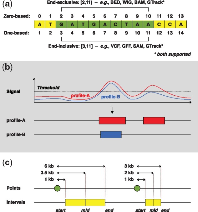
(a) Examples of coordinates of a sequence of nucleotides on zero-based and one-based genome coordinate systems. The brackets represent closed while parentheses represent open intervals. Being closed at a position represents the inclusion of that position in the genomic interval, whereas being open represents the exclusion of that position. (b) Example of discretizing continuous value to call genomic intervals. Here, although both profile-A and profile-B look visually similar, one of the genomic intervals in profile-B was not called because of marginally falling below a chosen threshold or owing to algorithm parameters, resulting in the exclusion of that region from further analyses. (c) Example of variations when computing distances from start, midpoint or end coordinates. Here, although both the points are 1 kb upstream of the genomic intervals, because of the differences in the length of genomic intervals the distances largely differ (here almost 2-fold) when computed to the midpoint or end
Continuous data associated with genomic sequences is often discretized into a set of high-valued genomic regions before analysis [as in e.g. peak calling of chromatin immunoprecipitation sequencing (ChIP-seq) data (Zhang et al., 2008)]. Since discretization reduces information (see an example in Fig. 1b), using the original continuous signal in statistical testing has the potential to improve statistical power. Both generic (Stavrovskaya et al., 2017) and technology-specific [e.g. Chen et al. (2015) and Shao et al. (2012)] methodologies have been proposed to correlate continuous signal of genomic tracks. Another solution to avoid the loss of data due to thresholding, is to incorporate some form of uncertainty associated with genomic regions (e.g. weights, P-values) into the descriptive measure of colocalization.
In certain analysis scenarios (e.g. when computing distances between genomic features), genomic regions may be represented by their start-, end- or mid-point, or may be expanded to include flanks. The choices of a reference point (start, midpoint or end), and flank sizes will provide alternative perspectives about the genomic features of interest (e.g. see Fig. 1c). Therefore, if reduction of transformation of data is required, one has to be conscious about their effects and interpretation.
Examples: https://hyperbrowser.uio.no/coloc/u/hb-superuser/p/data-representation-1
3 Avoid using a single fixed resolution if there is no good biological reason for it
Deoxyribonucleic acid (DNA) sequence properties and genomic features are often scale-specific, and they may thus appear differently when measured at different scales (Supplementary Fig. S1). The strength of statistical association observed between genomic features may thus vary when observed across multiple scales. To avoid misconceptions, the choice of scale ought to reflect the intrinsic scale at which the biological phenomena occur. Therefore, analysis of scale-specific events should either be guided by a knowledge-driven choice of the resolution or through rigorous investigation at multiple scales.
A common strategy in the analysis of genomic elements is to apply binning of genomic elements into multiple windows of predefined size, in order to obtain window-level statistics. However, it is known that the density of functional elements varies along the chromosomes. For example, focused genetic variation such as single nucleotide polymorphisms (SNPs) and insertions or deletions (InDels) occurs on a scale of a single base or a few bases; transcription factor binding sites determined through ChIP-seq typically span ∼100 bases; RNA transcripts and broad genetic variation, like copy number variations (CNVs), typically occur on a scale of kilo bases; and recombination regions can span several megabases. A priori selection of window size is thus a reasonable approach when prior knowledge exists about the resolution of the genomic event of interest. Without prior knowledge, however, using a single fixed window size can lead to a loss of statistical power and misleading conclusions.
For many research questions, the biological resolution of a genomic event of interest is not known. Therefore, an alternative to drawing conclusions based on an arbitrary window size could be to analyze the correlations between tracks at multiple scales to identify the scale-specific relationship between biological processes of interest. A few studies have previously tackled this problem by employing techniques routinely used in image processing and segmentation. For example, wavelet-transforms have been used to transform the observed signal intensity in a way that captures the variation in the data at successively broader scales. By correlating the transformed signal at each scale, the scale-specific interactions between biological processes of interest have been evaluated (Chan et al., 2012; Liu et al., 2007; Spencer et al., 2006). With the same objective, multiscale signal representation, which is routinely used in image segmentation, has been applied to genomic signals to convolve the genomic signal into segments at successive scales to capture the unknown scale variations of the signal (Knijnenburg et al., 2014). Recently, Gaussian kernel correlation has been proposed to correlate continuous data generated in genomics experiments (Stavrovskaya et al., 2017). Although the method was intended for correlating continuous data, the underlying idea is to avoid binning of continuous data into windows of arbitrarily-chosen size. The overarching theme of all these methods is to smoothen the observed signal, capturing the regional variation and subsequently to perform spatial correlation. This is equivalent to assessing correlations at several different scales that are successively broader.
Overall, a reasonable choice of window size would depend on the research question, and the choice should be based upon the type of genomic feature under study. Similar ideas are appropriate when choosing a reasonable length of flanking sequences where previous experimental evidence is not available.
Examples: https://hyperbrowser.uio.no/coloc/u/hb-superuser/p/predefined-resolution
4 Choose an appropriate test statistic and a suitable measure for effect size
In colocalization analysis, the pairwise relation of two tracks is summarized using a test statistic. The test statistics used in colocalization analyses are based on counts, distances or overlap. Examples of these metrics include the total number of intersecting genomic intervals between two tracks (counts), the total number of bases overlapping between the intersecting elements of two tracks (overlap) and some form of distance (average or geometric) between the closest elements. It has even been proposed to exchange the overlap/distance value of each individual genomic interval with a P-value that denotes its proximity to the genomic elements of a second track (Chikina and Troyanskaya, 2012). Adding P-values in this way will in effect scale the per-interval proximity values by what distance would be expected by chance, and allow subsequent direct interpretation of the distribution of computed P-values. While most of the existing colocalization analysis tools based on exact tests use a count statistic, Monte Carlo (MC) simulations-based tools make use of other test statistics as well.
The precise formulation of a research question reflects a specific choice of test statistic in MC simulation-based methods. As an example, let us consider the choice of test statistic when investigating whether genome-wide association study (GWAS) -implicated SNPs preferentially lie in the proximity of annotated genes. One way to formulate this question is as follows: do the SNPs fall inside protein-coding genes more frequently than expected by chance? This formulation would suggest using a count-based test statistic. However, one could also ask whether SNPs are preferentially located in gene-rich regions. One possible test statistic could then be based on expanding the SNP locations with large flanks on both sides, followed by an assessment of whether the overlap between these expanded regions and genes is higher than expected by chance. A third possibility is to ask whether the SNPs are generally close to genes. The test statistic could then be based on determining the closest gene of each SNP, computing the geometric or arithmetic average of these distances (respectively emphasizing immediate or moderate proximity), and assessing whether this average is different from what would be expected by chance. Notably, all the above formulations have an asymmetric aspect, meaning that the observations and the conclusions may change depending upon the direction of analysis. The inverse formulations—whether genes fall inside SNPs, whether genes are located in SNP-rich regions or whether genes are generally close to SNPs—appear less meaningful biologically.
In all the above formulations, the test statistic describes the relation of interest. However, in the majority of cases, the test statistic does not serve as an effective metric to understand the size of the effect. For instance, a statistically significant overlap of 1000 base pairs between a pair of tracks does not directly reveal whether or not the observed overlap is of sufficient magnitude that it could plausibly have biological consequences. Therefore, certain descriptive measures can be used to quantify effect size, supporting biological data interpretation. A widely used measure of effect size is the ratio between the observed value of the test statistic compared to the expected value (typically as a ratio of observed to expected).
Examples: https://hyperbrowser.uio.no/coloc/u/hb-superuser/p/test-statistic
5 Remember that all statistical tests are limited by the realism of the assumed null model
Statistical hypothesis testing has been one of the main approaches to assess whether the observed colocalization between two genomic features is likely to have occurred only because of chance. In this approach, it is hypothesized that the genomic features being tested occur independently along the genome (null hypothesis, H0), and the probability of the observed colocalization, or something more extreme, is computed (i.e. the P-value). The P-value is computed by comparing the observed test-statistic (e.g. overlap, distance, counts) with the background distribution of a test statistic, which is obtained through a model that assumes that null hypothesis is true (i.e. the null model). The null model should appropriately model the distributional properties and dependence structure of the genomic features along the genomic sequence (Fig. 2). Essentially, the aim is to as closely as possible preserve the characteristics of each genomic track in isolation, while at the same time nullifying any dependence between the two genomic tracks (because they are assumed to be independent in H0).
Fig. 2.

Examples of the distributional properties and dependence structure of genomic features along the genomic sequence. Genomic tracks contain genomic regions that are known to occur in clumps and with variable lengths. Also, genomic sequences could be characterized by the distributional and biological properties of genomic events, where stretches of sequence share similar biological properties (as homogeneous blocks). Furthermore, multiple genomic annotations colocalize with each other and thus any statistical association should disentangle the effect mediated by the colocalization of confounding features
All the statistical tests assume some form of null model that can range from being too simplistic to being too cautious. The conclusions of colocalization analysis would vary depending upon the choice of null model, where too simplistic null models give over-optimistic findings (Ferkingstad et al., 2015). Therefore, understanding the assumptions of the null model will help the researcher to assess whether the assumptions are appropriate for their data. This will allow the researcher to make an informed choice and to avoid false positives.
To grasp the implications of a given null model, it is useful to consider i) which properties of the real data are preserved in the null model, and ii) how the remaining properties are distributed (Sandve et al., 2010). A null model could for instance preserve the number of elements in each track, some distributional properties of each track (e.g. clumping tendency), or the tendency of each track to have more occurrences in certain parts of the genome (e.g. certain chromosomes). Consider an example case of a colocalization test between the binding sites of two transcription factors (TFBS). Suppose that the null model of choice preserves the number of TFBS in each track, but assumes that the TFBS are uniformly distributed across the genome. By understanding the assumptions of the null model, the researcher can assess whether this is a reasonable assumption given the known clumping tendencies of TFBS (Haiminen et al., 2008).
6 Make an informed choice about the most suitable null model
The null models that are routinely used in colocalization analysis can broadly be categorized into two types (Fig. 3). They are (i) the general null models of co-occurrence based either on analytical determination or Monte Carlo (MC) simulations, and (ii) the ones that use an explicit set of background or ‘universe’ regions to contrast the observed level of colocalization between a pair of genomic tracks (using e.g. a hypergeometric distribution). This categorization is described in detail in Box 1, together with descriptions on the statistical methodologies and assumptions, and a discussion on the advantages and disadvantages of each method. Below, we briefly provide a set of recommendations to aid the choice of appropriate null models.
Fig. 3.

The statistical methods for colocalization analysis can broadly be categorized into two types depending upon whether they use (a) a general null model of colocalization (b) or a specifically selected set of universe regions to estimate a null model (upper and lower panels). Both methods are further categorized as either (i) analytical tests (ii) or tests based on Monte Carlo simulations (left and right panels). Upper left: analytical tests with a general null model is exemplified by a binomial test on whether Track 1 (T1) positions are located inside Track 2 (T2) regions more than expected by chance. Upper right: General Monte Carlo-based tests provide great flexibility in the choice of test statistics and randomization strategies (null model). Here, exemplified by a simple overlap statistic (bps overlap) and uniform randomization of T2. Lower left: A set of universe regions limits the analysis to (here) the ‘case’ regions of T1 and a set of ‘control’ regions that could have been part of T1. Simple counting of the overlapping regions in T1 and T2 provides the basis of a Fisher's exact test. Lower right: The combination of universe regions and Monte Carlo-based testing is not previously presented in literature, but might be designed to combine advantages of them both. For a detailed overview of the null model categories, see Box 1
6.1 Use a simple analytical test only if the typically simple null model is acceptable
Simple analytical tests typically assume a simple null model as exemplified in Box 1 by Fisher’s exact test. When using simple analytical tests, one should be conscious of whether the null model fits with the data, and if not, how robust the test is to handle such violations. Assuming a too simple null model has been found to result in smaller P-values and thus more false positives (Ferkingstad et al., 2015). A recent study has reported a good correlation between the P-values obtained through a Fisher’s exact test (contingency table filled with per-interval counts) and MC simulations (Layer et al., 2018). However, the MC simulations reported in that study were based on a simple permutation model of uniform distribution of genomic intervals (Layer et al., 2018), which can lead to strong over-estimation of statistical significance (De et al., 2014; Sandve et al., 2010).
6.2 Consider using a MC-based hypothesis testing with a realistic (non-uniform) null model
Approaches based on MC simulations are computationally intensive and may require careful customization. As discussed in Box 1, the degree of preservation of the data characteristics in a null model affects the conclusions obtained through MC simulations. Previous case studies have shown that the higher the preservation of data characteristics in null models, the lower the statistical significance (larger P-values) (Ferkingstad et al., 2015). However, it is also recommended to assess the consistency of conclusions with different choices of null model to avoid being blindly conservative (De et al., 2014). A null model that aptly captures the randomness while mimicking the real complex nature of the genome would be an ideal choice. The development of such a model is far from trivial. The genomic sequence could be perceived as a frozen state of evolution, consisting of a large number of rare events over time. A considerable proportion of such stochastic events may depend on the previous rare events in evolution that might be predictable from a sequence analysis perspective. This points to comparative genomics as a potentially powerful approach to characterize the randomness of genome.
6.3 Use analytical tests based on a set of universe regions, if it flows naturally from the analysis domain, but construct the control set with great care
The use of a universe of genomic regions represents both an advantage and a disadvantage. As an example, when analyzing a set of SNPs, it could be useful to define the full set of common SNP locations as universe regions. In settings where such universe regions can be readily constructed, it simplifies the statistical assessment and offers high flexibility in the null model, for instance by supplying a universe set that matches the genomic track in terms of potentially confounding genome characteristics. However, the specification of a control set must be done with great care. Discrepancies between the case and control sets in various properties of the data (such as genomic heterogeneity and clumping) might easily in itself break the assumptions of the analytical test, possibly leading to false positives.
Examples: https://hyperbrowser.uio.no/coloc/u/hb-superuser/p/null-models
7 To avoid false positives use null models that account for local genome structure
The genome organization is complex, with several interdependencies. Various genomic elements and sequence properties occur along the genome in a non-uniform and dependent fashion (Gagliano et al., 2014; Kindt et al., 2013; Zhang et al., 2007), leading to various local heterogeneities in the genomic sequence (see Fig. 2). A track-level similarity measure or summary statistic may conceal such heterogeneity. Some few tools have tried to handle this issue by computing summary statistics in user-defined or fixed-size windows along the genome. However, this approach is again problematic because of the inherent problems of predefining the window sizes (discussed above in Section 2). Statistical testing that does not preserve the local genomic structure may lead to spurious findings of association or enrichment (Bickel et al., 2010). As an example, consider the case of assembly gaps in the physical maps of the genomes (International Human Genome Sequencing Consortium, 2004; Treangen and Salzberg, 2012). It has recently been shown that ignoring to account for assembly gaps (spanning around 3–6% of the total genome size) can lead to a higher degree of false findings (Domanska et al., 2018). On the other hand, in a typical MC simulations-based approach, too much preservation of the local genomic structure will result in too little randomness and in poor P-value estimates. A few tools provide the functionality to preserve the local genomic structure either by restricting the randomizations to regions matched by the local genomic properties [e.g. Heger et al. (2013), Quinlan and Hall (2010) and Sandve et al. (2010)], or by defining an explicit background set matched by local genomic properties (Dozmorov et al., 2016; Gel et al., 2016; Sheffield and Bock, 2016). In addition, a few SNP-centric tools match the genomic locations of SNPs with a selection maintaining properties such as gene density, minor allele frequency, number of SNPs in linkage disequilibrium (LD) and proximity to transcription start and end sites. Although matching of the SNP locations based on the above parameters will not be sufficient to control the false-positive rates, matching at least by the number of SNPs in LD has been shown to be critical for appropriate statistical performance (Trynka et al., 2015). A similar bias arises because of the intrinsic nature of some of the technology platforms, like genotyping arrays, which vary greatly in the number of probed markers and the physical distribution of these within the genome. Not accounting for these differences when generating the null distributions could also lead to false interpretations.
Nevertheless, one of the main challenges of matching by genomic properties is that it requires prior knowledge about all the genomic properties that would otherwise confound the observations when not appropriately matched. An alternative solution to handle this challenge is to restrict the testing space to the local site (for example restricting the distribution of the information elements being tested to locally homogenous blocks as in Fig. 4d). Several approaches have been proposed for handling this issue. The first approach implemented in several tools, allows the users to restrict the analysis space to user-supplied or dynamically-defined genomic regions [e.g. in Heger et al. (2013), Sandve et al. (2010), Sheffield and Bock (2016) and Trynka et al. (2015)]. In MC-simulations-based approaches, this functionality could be used to restrict the shuffling of genomic intervals to user-supplied regions that are matched by local genomic properties, whereas approaches that explicitly require a background set of regions could construct the background set to match the local genomic properties. While the simplest and most typical way of restricting the analysis space is based on a discrete decision of whether or not to include a given region, it is also possible to provide a continuous (probabilistic) value for the inclusion of a given region or base pair (Sandve et al., 2010). An alternative approach (Bickel et al., 2010) uses segmentation to segregate the locally homogeneous regions of the genome. Subsequently, random blocks of homogenous regions are subsampled within the segments to estimate a confidence interval of colocalization. With this method, the biologist has to make essential choices in some aspects like the scale of segmentation, and the subsample size, that would affect the statistical conclusions.
Fig. 4.
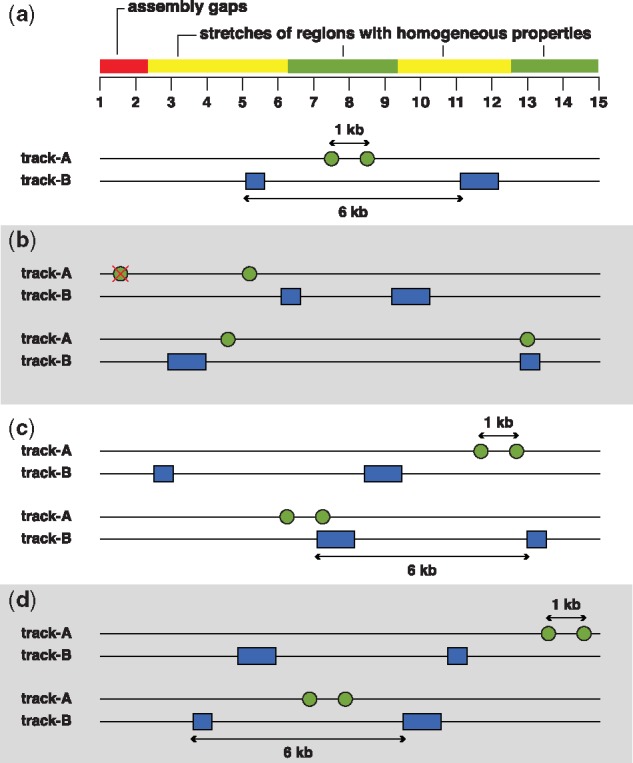
Examples of different permutation strategies in Monte Carlo Null models. (a) In this illustration, let us assume that the dependence relationship between track-A and track-B is being queried. Note the local heterogeneities within the genomic region, where blue and green segments represent blocks of locally homogenous regions. The red segment represents assembly gaps. Tracks A and B are comprised of points and genomic intervals respectively, and different colors are used to distinguish them. (b) The simplest form of permutation model assumes uniformity and independence of genomic locations and thus shuffles either of the track without any restrictions. Note here that one of the points was also shuffled to an assembly gap region. (c) Another null model preserves the sequence distance between the points or genomic intervals when shuffling and avoids gaps. (d) A more conservative strategy preserves the sequence distance, while also shuffling to regions matched by biological properties (blue and green colors) thus preserving local heterogeneity
Examples: https://hyperbrowser.uio.no/coloc/u/hb-superuser/p/local-genomic-structure
8 Consider potential confounding features and control for their effects
A statistically significant correlation between two functional genomic elements may in fact be driven by colocalization with another (known or unknown) third genomic element or sequence property (in some cases unknown) that was not included in the analysis (see Fig. 2). Spatial dependencies exist for a number of genomic elements. For example, a significant fraction of copy number variation occurs in proximity to segmental duplications (Sharp et al., 2005); non-coding variants are concentrated in regulatory regions marked by DNase I hypersensitive sites (DHSs) (Maurano et al., 2012); DHS exons are enriched near promoters or distal regulatory elements (Mercer et al., 2013); higher gene density is found in GC content-rich regions (Lander et al., 2001); and extensive pairwise overlap is often found between the binding sites of transcription factors that co-occur and co-operate (Zhang et al., 2006). Not testing for the association of potential confounding factors (e.g. GC content, overlap with repetitive DNA, length of the genomic intervals, genotype and other genetic factors) might thus lead to incomplete or erroneous conclusions. When the colocalization of a pair of genomic features is confounded by a third genomic feature, one could unravel the specific relations by contrasting the pairwise overlap statistics or enrichment scores of all the three features.
Below are two examples that handled confounding factors by including them into the null model. Trynka et al. (Trynka et al., 2015) used stratified sampling where the track to be randomized is divided into two sub-tracks defined by either being inside or outside regions in the confounding track. The sub-tracks are then individually randomized. However, as with any stratified analysis, this may result in the loss of statistical power. Another example based on MC simulations handled the potential confounding relation between two tracks by shuffling the genomic locations according to a non-homogenous Poisson process, where the Poisson parameter depended on the locations defined in a third (or several) co-localizing genomic tracks (Sandve et al., 2010).
Examples: https://hyperbrowser.uio.no/coloc/u/hb-superuser/p/confounding-features
9 Use additional methods to test the validity of the conclusions
One of the major harms of false-positive findings in colocalization analysis (or in any genomic analysis) is the triggering of futile follow-up projects (MacArthur, 2012). When relying on the conclusions of colocalization analysis to plan follow-up experiments, one might therefore find it beneficial to have an additional validation step to test whether some form of biases have crept into the analysis. Such validation can be performed by simulating artificial data of pairs of genomic tracks with no significant relationship (i.e. occurring independently of each other), and check whether the devised analytical methodology then results in a uniform distribution of P-values. [e.g. see Fig. 1 in Storey and Tibshirani (2003) and Altman and Krzywinski (2017)].
10 Summary and outlook
In the preceding sections, we provided guidelines for performing statistical colocalization analysis, which is routinely employed to understand the interplay between the genomic features. We highlighted the methodological challenges involved in each step of the colocalization analysis and discussed the existing approaches that can handle those challenges, when available. The state-of-the-art methodology for statistical analyses of colocalization vary in the comprehensiveness of handling such challenges. Moreover, ad hoc implementations of project-specific methodologies, which are common in biology-driven collaborative projects, may not necessarily handle all the challenges discussed above to a reasonable extent. Therefore, there is a need for the development of a unified and generic methodology that handles several of the potential shortcomings discussed here.
To avoid misinterpretation of the conclusions in colocalization analyses, it is essential to be aware of the pitfalls discussed in this article. In addition, as with any application of statistical hypothesis testing, it is also highly recommended to consider the effect size in addition to P-values. There has lately been considerable focus on the fallacies of blindly drawing conclusions from a P-value (Halsey et al., 2015; Nuzzo, 2014). This is particularly important in situations with very large datasets, which is often the case in genome analysis, since even a minor deviation from the null hypothesis may be statistically significant (without obvious biological relevance). It is thus recommended to apply measures that combine effect size and precision, such as confidence intervals, or by filtering, ranking or visualizing results based on a combination of P-values and their corresponding effect sizes (e.g. using volcano plots).
False findings in colocalization analysis could be avoided by being aware of the accumulated knowledge on best methodological practices. The accumulated knowledge can be categorized into two layers: (i) First, a generic layer represented by all the guidelines detailed in this manuscript, and (ii) second, a specific layer represented by the data type-specific particularities. One of the main examples of such data type-specific particularities is the genomic properties that are to be matched when drawing samples for the null (e.g. LD for SNPs, chromatin accessibility levels and GC content for transcription factor footprinting and so on). In this example, which properties are to be matched would depend on both the annotations being tested and can also be unknown in several cases. In such cases, simulation experiments as suggested in Section 9 of this article could be performed to test and evaluate the potential biases that could inflate the false findings.
While the existing tools are focused on a simple linear sequence model of the reference genome, there are ongoing efforts to represent reference genomes in a graph structure to better represent the sequence variation and diversity (Church et al., 2015; Paten et al., 2017). Novel coordinate systems are being proposed for the better representation of genomic intervals on a graph structure (Rand et al., 2017). As the preliminary evidence suggest that the genome graphs improve read mapping and subsequent operations like variant calling (Novak et al., 2017), we anticipate that the accuracy of colocalization analyses would also improve as a consequence. The future tool development in colocalization analyses should be tailored towards handling genome graphs, pending the availability of a universal coordinate system and exchange formats.
Another recent development is single-cell sequencing, which is now beginning to extend beyond RNA-seq to also include other -omics assays. It is being increasingly acknowledged that explicit phenotype-genotype associations could be established by integrating multiple omics features from the same cell (Bock et al., 2016; Macaulay et al., 2017). The inherent limitation of single cell sequencing technology in generating low coverage, sparse and discrete measurements (as of now) however affects the statistical power in detecting true associations between multiple omics features. One way of overcoming the low statistical power is by aggregating the signal across similar functional elements (e.g. aggregating expression levels of functionally similar genes) (Bock et al., 2016; Farlik et al., 2015). Apart from overcoming the inherent challenges of single cell sequencing technology, colocalization analysis is one of the suitable ways to integrate multiple omics features, especially due to the ripe methodologies that can appropriately model the genomic heterogeneities.
Supplementary Material
Acknowledgements
We thank Boris Simovski for critical reading of the manuscript.
Box 1. Null models and statistical tests of colocalization
This section provides a categorization of statistical tests of colocalization and the associated null models into four subtypes, as illustrated in Figure 3. The statistical tests differ on whether they make (a) use of a general null model of colocalization or (b) a specifically selected set of universe regions to estimate a null model. Further they can be classified as (i) analytical tests or (ii) tests based on Monte Carlo simulations:
(a) Colocalization analysis methods based on general null models
(i) Analytical tests
Analytical tests are either parametric or non-parametric. Parametric tests assume that the data is sampled from a population that follow a particular probability distribution as described by a set of parameters, e.g. the mean and variance of a normal distribution. Individual genomic tracks typically contain genomic regions of variable lengths (number of base pairs covered) that are often dependent on each other, for instance by occurring in clumps along the genome, as illustrated in Figure 2 (Bickel et al., 2010; Haiminen et al., 2008; Sandve et al., 2010). Therefore, the challenge of using parametric tests for colocalization analysis lies in finding a parametric distribution of colocalization that reflects the variable lengths, clumping nature and other dependency structures of the genomic features. Violating the assumptions on the probability distribution invalidates the results, although it depends on the distribution and the type and extent of violating to what degree the results may still be informative and interpretable.
Non-parametric tests, on the other hand, do not assume any a priori distribution, and are thus typically more robust (but with less statistical power). For instance, a tempting straightforward non-parametric test would be a Fisher’s exact test, which is an often-used test of colocalization [e.g. Roadmap Epigenomics Consortium et al. (2015)]. Fisher's exact test operates on observations allocated to two different categories, and tracks all combinations of categories in a 2x2 contingency table. When testing the significance of colocalization between a query track and reference track, the 2x2 contingency table for Fisher’s exact test typically consists of (a) co-occurrences of query and reference track, (b) occurrences solely for query track, (c) occurrences solely for reference track and (d) occurrences for neither query nor reference tracks. With such an approach, the first challenge is to quantify co-occurrence in such a way as to also allow counting of lack of occurrences. A second challenge is that the Fisher’s exact test assumes in the null hypothesis that each counted observation is independently allocated to the categories. Counting coverage per base pair is a straightforward way to meet the first challenge, but will in the usual cases lead to an extreme dependence between observations (due to consecutive base pairs being covered by the same element). It is therefore necessary to discretize occurrence and co-occurrence to per-interval counts or to per-fixed-window counts, which comes with reduced resolution and still it ignores the widespread clumping of elements in the genome.
Fisher's exact test assumes that the column and row totals are fixed, which in the context of colocalization analysis means that the total number of observations (base pairs, regions or fixed-size windows) in the query and reference sets are preserved. However, other properties of the data like region lengths, clumping tendencies, local heterogeneity or other confounders are not preserved in the method itself, and such properties are likely to create dependencies in the allocation of categories to the observations.
In brief, non-parametric tests are not assumption-free, they are still limited by whether the assumptions are met by the data and experiment conditions.
(i) Tests based on Monte Carlo simulations
In a typical Monte Carlo (MC) simulations-based approach, a null model will be used to repeatedly generate sample data, which is then used to calculate the distribution of the test statistic. The test statistic distribution will be utilized to estimate the P-value empirically as the proportion of
extreme test statistics (number of test statistics that are equal to or larger than the observed test statistic) (Fig. 3). Monte Carlo simulations provide high flexibility in terms of selecting appropriate test statistics and null models (even as two mostly independent choices), albeit at high computational cost (Fig. 4a).
The simplest form of permutation model randomly shuffles the genomic locations along the genome, inappropriately assuming uniformity and independence along the genome (Fig. 4b). The definitions of other permutation models vary to a great degree in terms of the essential geometric and biological properties they retain from the observed data, and how the remaining properties are randomized (Fig. 4c and d). Some of the common choices to be made when choosing a permutation strategy are whether to preserve the interval lengths and clumping tendencies (distances), whether to allow or disallow overlaps among the shuffled locations, whether to restrict the shuffling to certain regions of the reference sequence (for instance, restricting by chromosomes or arms and avoiding assembly gaps; see Fig. 2). Shuffling by allowing overlaps when the real data does not contain overlaps, and vice versa, may result in a null model that is not representative of the observed data. The degree of preservation of the data properties thus obviously affect the statistical conclusions.
(b) Colocalization analysis based on a specifically selected set of universe regions
(i) Analytical tests
Another approach of colocalization analysis requires defining a set of universe regions from the outset to estimate a null model. The universe set is comprised of the actual ‘case’ regions in the track being queried for colocalization, in addition to a set of ‘control’ regions selected somehow in negation to the case regions. Ideally, the full universe set is comprised of all the regions that could have possibly ended up in the genomic tracks being queried for colocalization (Sheffield and Bock, 2016). As an example, when testing the colocalization of a SNP set with other annotations, the background set could be all the SNPs covered by the technology platform, which are all assumed to have equal probability to be included in the SNP set of interest.
Specifically defining a universe makes it less problematic to use analytical tests, as a carefully chosen universe makes it easier to follow the assumptions of an analytical test. This is exemplified in the following with Fisher’s exact test. As detailed under point (a, i) Fisher's exact test operates on observations that can fall within two different binary categories, here whether a region is a case or a control region and whether it overlaps the reference track or not. Note again that the Fisher’s exact test in itself preserves very little of the properties of the data, only the total number of observations in each of the two categories. Large discrepancies between the case and control regions for other properties, like the lengths of the regions or their clumping tendencies along the genome, could break the null hypothesis that the observations are allocated independently into the two categories, and thus invalidate the test. The important issue is whether such discrepancies in themselves break the null hypothesis that the observations are allocated independently into the two categories. If for instance, the case regions are larger than the control regions, they are more likely to overlap the reference regions only due to their length. Another example is if both case and reference regions favour areas of open chromatin, while the control set is selected without this in mind. In both cases the Fisher's exact test might correctly report significance, i.e. that the null hypothesis does not hold, but this will just be due to deficiencies in the experiment conditions and the result will not be biologically relevant. Thus, the set of control regions must be carefully selected to match the properties of the case regions in terms of e.g. region lengths, clumping tendencies, local genome structure and confounding factors (as described elsewhere in this paper).
In brief, when combining an analytical test with estimating a null model by selecting a set of universe regions, the definition of a realistic null model is ‘outsourced’ from the method (the statistical test) to the universe selection process carried out by the user. If this selection is not done carefully, the results will typically be overly optimistic and produce false positives.
(ii) Tests based on Monte Carlo simulations
The combination of Monte Carlo simulation with estimating a null model from a set of universe regions is, to our knowledge, not used in any published methods for colocalization analysis. Theoretically, the combination might be used to alleviate some of the possible issues of using analytical tests. Monte Carlo simulation allows careful delineation of the randomization process, allowing the preservation of properties such as region lengths and clumping tendencies in the method itself, simplifying the process of selecting a set of universe regions. The obvious drawback is increased computational time.
Funding
Stiftelsen Kristian Gerhard Jebsen (K.G. Jebsen Coeliac Disease Research Centre). Austrian Academy of Sciences New Frontiers Group Award and ERC Starting Grant (European Union’s Horizon 2020 research and innovation programme) 679146 to CB.
Conflict of Interest: none declared.
References
- Altman N., Krzywinski M. (2017) Points of significance: P values and the search for significance. Nat. Methods, 14, 3–4. [DOI] [PMC free article] [PubMed] [Google Scholar]
- Bickel P.J. et al. (2010) Subsampling methods for genomic inference. Ann. Appl. Stat., 4, 1660–1697. [Google Scholar]
- Birney E. et al. (2007) Identification and analysis of functional elements in 1% of the human genome by the ENCODE pilot project. Nature, 447, 799–816. [DOI] [PMC free article] [PubMed] [Google Scholar]
- Bock C. et al. (2009) EpiGRAPH: user-friendly software for statistical analysis and prediction of (epi)genomic data. Genome Biol., 10, R14.. [DOI] [PMC free article] [PubMed] [Google Scholar]
- Bock C. et al. (2016) Multi-omics of single cells: strategies and applications. Trends Biotechnol., 34, 605–608. [DOI] [PMC free article] [PubMed] [Google Scholar]
- Chan A.H. et al. (2012) Genome-wide fine-scale recombination rate variation in Drosophila melanogaster. PLoS Genet., 8, e1003090. [DOI] [PMC free article] [PubMed] [Google Scholar]
- Chen L. et al. (2015) A novel statistical method for quantitative comparison of multiple ChIP-seq datasets. Bioinformatics, 31, 1889–1896. [DOI] [PMC free article] [PubMed] [Google Scholar]
- Chikina M., Troyanskaya O. (2012) An effective statistical evaluation of ChIPseq dataset similarity. Bioinformatics, 28, 607–613. [DOI] [PMC free article] [PubMed] [Google Scholar]
- Church D.M. et al. (2015) Extending reference assembly models. Genome Biol., 16, 13.. [DOI] [PMC free article] [PubMed] [Google Scholar]
- Conway J.R. et al. (2017) UpSetR: an R package for the visualization of intersecting sets and their properties. Bioinformatics, 33, 2938–2940. [DOI] [PMC free article] [PubMed] [Google Scholar]
- De S. et al. (2014) The dilemma of choosing the ideal permutation strategy while estimating statistical significance of genome-wide enrichment. Brief. Bioinform., 15, 919–928. [DOI] [PMC free article] [PubMed] [Google Scholar]
- Domanska D. et al. (2018) Mind your gaps: overlooking assembly gaps confounds statistical testing in genome analysis. doi:10.1101/252973. [DOI] [PMC free article] [PubMed] [Google Scholar]
- Dozmorov M.G. (2017) Epigenomic annotation-based interpretation of genomic data: from enrichment analysis to machine learning. Bioinformatics, 33, 3323–3330. [DOI] [PubMed] [Google Scholar]
- Dozmorov M.G. et al. (2016) GenomeRunner web server: regulatory similarity and differences define the functional impact of SNP sets. Bioinformatics, 32, 2256–2263. [DOI] [PMC free article] [PubMed] [Google Scholar]
- Farlik M. et al. (2015) Single-cell DNA methylome sequencing and bioinformatic inference of epigenomic cell-state dynamics. Cell Rep., 10, 1386–1397. [DOI] [PMC free article] [PubMed] [Google Scholar]
- Favorov A. et al. (2012) Exploring massive, genome scale datasets with the GenometriCorr package. PLoS Comput. Biol., 8, e1002529. [DOI] [PMC free article] [PubMed] [Google Scholar]
- Ferkingstad E. et al. (2015) Monte Carlo null models for genomic data. Stat. Sci., 30, 59–71. [Google Scholar]
- Gagliano S.A. et al. (2014) A Bayesian method to incorporate hundreds of functional characteristics with association evidence to improve variant prioritization. PloS One, 9, e98122. [DOI] [PMC free article] [PubMed] [Google Scholar]
- Gel B. et al. (2016) regioneR: an R/Bioconductor package for the association analysis of genomic regions based on permutation tests. Bioinformatics, 32, 289–291. [DOI] [PMC free article] [PubMed] [Google Scholar]
- Goodwin S. et al. (2016) Coming of age: ten years of next-generation sequencing technologies. Nat. Rev. Genet., 17, 333–351. [DOI] [PMC free article] [PubMed] [Google Scholar]
- Haiminen N. et al. (2008) Determining significance of pairwise co-occurrences of events in bursty sequences. BMC Bioinformatics, 9, 336.. [DOI] [PMC free article] [PubMed] [Google Scholar]
- Halachev K. et al. (2012) EpiExplorer: live exploration and global analysis of large epigenomic datasets. Genome Biol., 13, R96. [DOI] [PMC free article] [PubMed] [Google Scholar]
- Halsey L.G. et al. (2015) The fickle P value generates irreproducible results. Nat. Methods, 12, 179–185. [DOI] [PubMed] [Google Scholar]
- Heger A. et al. (2013) GAT: a simulation framework for testing the association of genomic intervals. Bioinformatics, 29, 2046–2048. [DOI] [PMC free article] [PubMed] [Google Scholar]
- Heinz S. et al. (2015) The selection and function of cell type-specific enhancers. Nat. Rev. Mol. Cell Biol., 16, 144–154. [DOI] [PMC free article] [PubMed] [Google Scholar]
- International Human Genome Sequencing Consortium. (2004) Finishing the euchromatic sequence of the human genome. Nature, 431, 931–945. [DOI] [PubMed] [Google Scholar]
- Kanduri C. et al. (2017) Genome build information is an essential part of genomic track files. Genome Biol., 18, 175.. [DOI] [PMC free article] [PubMed] [Google Scholar]
- Khan A., Mathelier A. (2017) Intervene: a tool for intersection and visualization of multiple gene or genomic region sets. BMC Bioinformatics, 18, 287.. [DOI] [PMC free article] [PubMed] [Google Scholar]
- Kindt A.S.D. et al. (2013) The genomic signature of trait-associated variants. BMC Genomics, 14, 108.. [DOI] [PMC free article] [PubMed] [Google Scholar]
- Knijnenburg T.A. et al. (2014) Multiscale representation of genomic signals. Nat. Methods, 11, 689–694. [DOI] [PMC free article] [PubMed] [Google Scholar]
- Lander E.S. (2011) Initial impact of the sequencing of the human genome. Nature, 470, 187–197. [DOI] [PubMed] [Google Scholar]
- Lander E.S. et al. (2001) Initial sequencing and analysis of the human genome. Nature, 409, 860–921. [DOI] [PubMed] [Google Scholar]
- Lawrence M. et al. (2013) Software for computing and annotating genomic ranges. PLoS Comput. Biol., 9, e1003118.. [DOI] [PMC free article] [PubMed] [Google Scholar]
- Layer R.M. et al. (2018) GIGGLE: a search engine for large-scale integrated genome analysis. Nat. Methods, 15, 123–126. [DOI] [PMC free article] [PubMed] [Google Scholar]
- Liu F. et al. (2007) The Human Genomic Melting Map. PLoS Comput. Biol., 3, e93. [DOI] [PMC free article] [PubMed] [Google Scholar]
- Luco R.F. et al. (2011) Epigenetics in alternative pre-mRNA splicing. Cell, 144, 16–26. [DOI] [PMC free article] [PubMed] [Google Scholar]
- MacArthur D. (2012) Methods: face up to false positives. Nature, 487, 427–428. [DOI] [PubMed] [Google Scholar]
- Macaulay I.C. et al. (2017) Single-cell multiomics: multiple measurements from single cells. Trends Genet., 33, 155–168. [DOI] [PMC free article] [PubMed] [Google Scholar]
- Makova K.D., Hardison R.C. (2015) The effects of chromatin organization on variation in mutation rates in the genome. Nat. Rev. Genet., 16, 213–223. [DOI] [PMC free article] [PubMed] [Google Scholar]
- Maurano M.T. et al. (2012) Systematic localization of common disease-associated variation in regulatory DNA. Science, 337, 1190–1195. [DOI] [PMC free article] [PubMed] [Google Scholar]
- Mercer T.R. et al. (2013) DNase I-hypersensitive exons colocalize with promoters and distal regulatory elements. Nat. Genet., 45, 852–859. [DOI] [PMC free article] [PubMed] [Google Scholar]
- Novak A.M. et al. (2017) Genome Graphs. doi: 10.1101/101378. [Google Scholar]
- Nuzzo R. (2014) Scientific method: statistical errors. Nat. News, 506, 150.. [DOI] [PubMed] [Google Scholar]
- Paten B. et al. (2017) Genome graphs and the evolution of genome inference. Genome Res., 214155, 116. [DOI] [PMC free article] [PubMed] [Google Scholar]
- Portela A., Esteller M. (2010) Epigenetic modifications and human disease. Nat. Biotechnol., 28, 1057–1068. [DOI] [PubMed] [Google Scholar]
- Quinlan A.R., Hall I.M. (2010) BEDTools: a flexible suite of utilities for comparing genomic features. Bioinformatics, 26, 841–842. [DOI] [PMC free article] [PubMed] [Google Scholar]
- Rand K.D. et al. (2017) Coordinates and intervals in graph-based reference genomes. BMC Bioinformatics, 18, 263.. [DOI] [PMC free article] [PubMed] [Google Scholar]
- Roadmap Epigenomics Consortium. et al. (2015) Integrative analysis of 111 reference human epigenomes. Nature, 518, 317–330. [DOI] [PMC free article] [PubMed] [Google Scholar]
- Sandve G.K. et al. (2010) The Genomic HyperBrowser: inferential genomics at the sequence level. Genome Biol., 11, R121. [DOI] [PMC free article] [PubMed] [Google Scholar]
- Shao Z. et al. (2012) MAnorm: a robust model for quantitative comparison of ChIP-Seq data sets. Genome Biol., 13, R16.. [DOI] [PMC free article] [PubMed] [Google Scholar]
- Sharp A.J. et al. (2005) Segmental duplications and copy-number variation in the human genome. Am. J. Hum. Genet., 77, 78–88. [DOI] [PMC free article] [PubMed] [Google Scholar]
- Sheffield N.C., Bock C. (2016) LOLA: enrichment analysis for genomic region sets and regulatory elements in R and Bioconductor. Bioinformatics, 32, 587–589. [DOI] [PMC free article] [PubMed] [Google Scholar]
- Simovski B. et al. (2017) GSuite HyperBrowser: integrative analysis of dataset collections across the genome and epigenome. Gigascience, 6, 1–12. [DOI] [PMC free article] [PubMed] [Google Scholar]
- Spencer C.C.A. et al. (2006) The influence of recombination on human genetic diversity. PLoS Genet., 2, e148.. [DOI] [PMC free article] [PubMed] [Google Scholar]
- Stavrovskaya E.D. et al. (2017) StereoGene: rapid estimation of genome-wide correlation of continuous or interval feature data. Bioinformatics, 33, 3158–3165. [DOI] [PMC free article] [PubMed] [Google Scholar]
- Storey J.D., Tibshirani R. (2003) Statistical significance for genomewide studies. Proc. Natl. Acad. Sci. USA, 100, 9440–9445. [DOI] [PMC free article] [PubMed] [Google Scholar]
- Treangen T.J., Salzberg S.L. (2012) Repetitive DNA and next-generation sequencing: computational challenges and solutions. Nat. Rev. Genet., 13, 36–46. [DOI] [PMC free article] [PubMed] [Google Scholar]
- Trynka G. et al. (2015) Disentangling the effects of colocalizing genomic annotations to functionally prioritize non-coding variants within complex-trait loci. Am. J. Hum. Genet., 97, 139–152. [DOI] [PMC free article] [PubMed] [Google Scholar]
- Zhang C. et al. (2006) A clustering property of highly-degenerate transcription factor binding sites in the mammalian genome. Nucleic Acids Res., 34, 2238–2246. [DOI] [PMC free article] [PubMed] [Google Scholar]
- Zhang Y. et al. (2008) Model-based analysis of ChIP-Seq (MACS). Genome Biol., 9, R137.. [DOI] [PMC free article] [PubMed] [Google Scholar]
- Zhang Z.D. et al. (2007) Statistical analysis of the genomic distribution and correlation of regulatory elements in the ENCODE regions. Genome Res., 17, 787–797. [DOI] [PMC free article] [PubMed] [Google Scholar]
Associated Data
This section collects any data citations, data availability statements, or supplementary materials included in this article.