Improving Sensitivity on Identification and Delineation of Intracranial Hemorrhage Lesion Using Cascaded Deep Learning Models

Abstract

Highly accurate detection of the intracranial hemorrhage without delay is a critical clinical issue for the diagnostic decision and treatment in an emergency room. In the context of a study on diagnostic accuracy, there is a tradeoff between sensitivity and specificity. In order to improve sensitivity while preserving specificity, we propose a cascade deep learning model constructed using two convolutional neural networks (CNNs) and dual fully convolutional networks (FCNs). The cascade CNN model is built for identifying bleeding; hereafter the dual FCN is to detect five different subtypes of intracranial hemorrhage and to delineate their lesions. Using a total of 135,974 CT images including 33,391 images labeled as bleeding, each of CNN/FCN models was trained separately on image data preprocessed by two different settings of window level/width. One is a default window (50/100[level/width]) and the other is a stroke window setting (40/40). By combining them, we obtained a better outcome on both binary classification and segmentation of hemorrhagic lesions compared to a single CNN and FCN model. In determining whether it is bleeding or not, there was around 1% improvement in sensitivity (97.91% [± 0.47]) while retaining specificity (98.76% [± 0.10]). For delineation of bleeding lesions, we obtained overall segmentation performance at 80.19% in precision and 82.15% in recall which is 3.44% improvement compared to using a single FCN model.

Introduction

Stroke is the second leading cause of death worldwide and occurs accidentally [1]. It is generally thought that there are two types of stroke. One is an ischemic stroke, which is caused by a blood clot blocking blood vessels. The second type is hemorrhagic stroke, most of which are results of blood vessel bursting or rupturing, caused mostly by hypertension, head injury, and trauma. Highly accurate and timely imaging assessment of a hemorrhagic stroke is essential for diagnostic decision and treatment in emergency rooms. Excluding hemorrhage by non-contrast computed tomography (NCCT) from all stroke-suspicious patients within 3–4.5 h of the stroke onset time is the fundamental step, as the administration of intravenous tissue plasminogen activator (IV-tPA) can lead to serious side effects to actively bleeding patient [2, 3].

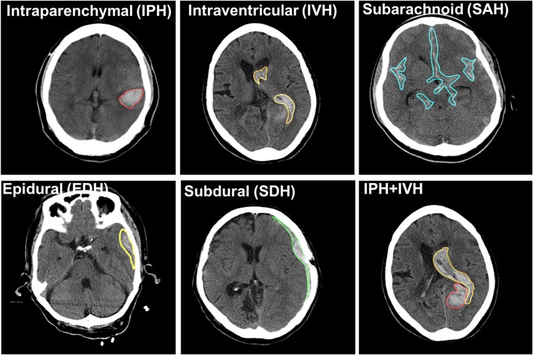
The intracranial hemorrhage is a life-threatening type of stroke. It is subcategorized into five types depending on its anatomical location and underlying causes. These subtypes are intraparenchymal hemorrhage (IPH), intraventricular hemorrhage (IVH), extradural hemorrhage (EDH), subdural hemorrhage (SDH), and subarachnoid hemorrhage (SAH) as shown in Fig. 1. While IVH bleeding occurs near a ventricle, EDH and SDH bleed at outer and inner of dural membranes. Patterns of the hemorrhagic lesion on CTs vary in shape and size, and they also develop a single or a mixture of several patterns. In conjunction with categorizing lesion patterns, estimating hemorrhage volume is another significant driving factor of 30-day mortality and morbidity. Consequently, highly accurate lesion segmentation of hematoma is another critical issue following the detection of hematoma [4]. However, certain factors or conditions such as signal to noise, signal attenuation, and artifacts may negatively influence recognizing the types of lesions and manual segmentation. This can lead to delayed diagnosis and misdiagnosis. Detecting intracranial hemorrhage and segmenting using a computer-aided detection or diagnosis (CAD)-based automatic system is a promising approach in improving workflow and reducing human errors. It results in a better patient outcome.

Fig. 1.

Five subtypes of intracranial hemorrhage on non-contrast computer tomography (NCCT)

Relevant works have presented various methods for automatic detection and delineation of hemorrhagic lesions on NCCT. For example, one method combines region-based active contour and fuzzy c-means to segment lesions [5], while another method proposes a random forest algorithm to achieve a fully automated segmentation approach [6]. However, these methods often demand complicated engineering feature including skull stripping, image registration, and feature extraction from voxel intensity and local moment information [7]. Recent deep learning technology enables the self-learning of nonlinear image filters and the self-extraction of relevant features [8]. The deep learning model constructed by convolutional neural networks (CNNs) is applied to identify the intracranial hemorrhage [9–13]. For the purpose of clinical triage studies, a 3D-CNN architecture was used to classify whether an image contained acute neurological illness or noncritical findings [14]. These papers only deal with simple binary classification problems of either normal or abnormal. Other recent works investigated both of the classification and segmentation but only handled three types of intracranial hemorrhage [15] and localization using bounding boxes [16]. To the best of our knowledge, there has not been any study on both five intracranial hemorrhagic identification and segmentation using a deep learning approach.

Accordingly, we propose a novel diagnostic system for segmentation as well as classification of intracranial hemorrhage. To detect subtle changes on CT images, we built a cascade architecture based on CNNs and dual fully convolutional networks (FCNs) for the purpose of classification and segmentation respectively. The idea was inspired by what radiologists do in order to find subtle changes by adjusting window width and center level of Hounsfield unit (HU), so that the contrast between normal and abnormal tissues can be accentuated. Using the combination of a default brain CT window setting (window level 50 HU/width 100 HU) and a stroke CT window setting (level 40 HU/width 40 HU) [17, 18] in cascade, it helps reduce false-negative cases and contributes to the improvement of sensitivity. We built a CNN cascade model and dual FCNs: the CNN cascade model was constructed to detect hemorrhage (bleeding) as a binary classifier. Once it is identified as bleeding, the dual FCN model is employed for identifying five subtypes of intracranial hemorrhage and segmenting their lesions.

Materials and Methods

Data Acquisition

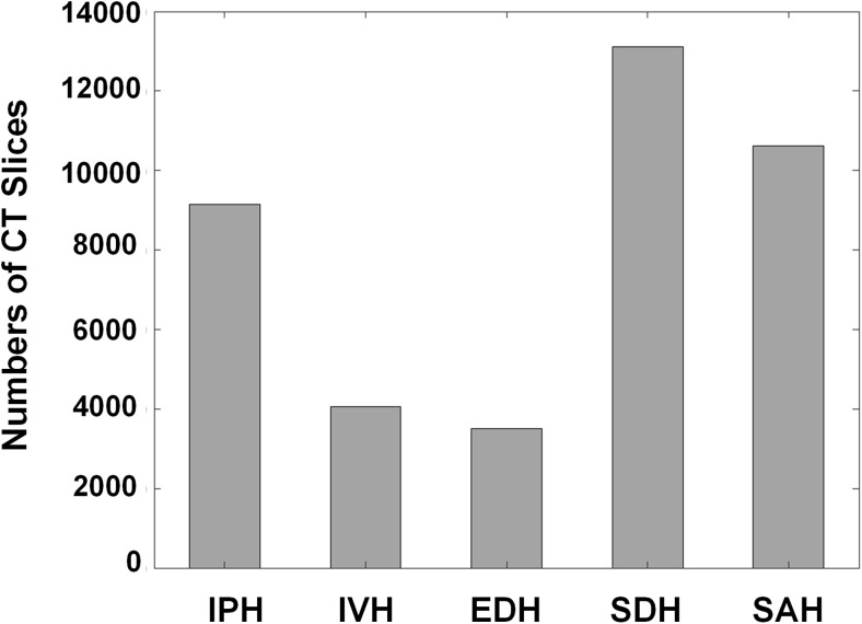
One hundred thirty-five thousand and nine hundred seventy-four non-contrast head CT images with 5 mm slice thickness from 5702 patients, of which 3055 cases were non-bleeding and 2647 cases were bleeding, were acquired from two institutes. The hemorrhagic patients were selected by ICD 10-based diagnosis codes including bleeding, traumatic and non-traumatic SAH, EDH, and SDH from 2011 to 2017. This data collection was reviewed and approved by the ethics committee at Kyungpook National University Hospital and Kyungpook National University Hospital Chilgok (KNUH 2017-06-005 and KNUCH 2016-11-050). Ten medical experts including one neurologist, four neurosurgeons, and five emergency medicine doctors participated to establish the ground truth labels. All of them have more than 10 years’ experiences in each department. After the patients’ sensitive information in DICOM files was anonymized, eight experts initially labeled all CT slices with an in-house annotation tool. And then the two senior experts with more than 5 years’ experiences in neurology subspecialty refined the initial-labeled ones in terms of false-negative and false-positive findings. The senior experts cross-checked the refined CTs and then the final ground truth labels were determined by consensus among all the experts. In case of bleeding, a total of 33,391 CT slices were well labeled by ten medical experts, also indicating the five subtypes of intracranial hemorrhage: intraventricular, intraparenchymal, subarachnoid, epidural, and subdural hemorrhage. Figure 2 shows the histogram of CT slices on five different types of hemorrhage so that we can identify how many CT image data accounts for each type of hemorrhage. Among a total of 2647 cases (33,391 slices), 1612 cases (61%) had only one ICH subtype and 1035 cases (39%) had at least two ICH subtypes.

Fig. 2.

Histogram of CT images on five intracranial hemorrhagic types: intraparenchymal (IVH), intraventricular (IPH), epidural (EDH), subdural (SDH), and subarachnoid hemorrhage (SAH)

Data Preprocessing

At the CT data preprocessing stage, the raw DICOM images were preprocessed by adjusting the window level (WL) and window width (WW). Through this stage, the Hounsfield unit (HU) numbers of a specified window ([WL-WW/2, WL+WW/2]) were transformed into a full range of grayscale values (0, 255). Each HU number was transformed by a specified window. Other HU values above (>WL+WW/2) and below (<WL-WW/2) window were set to be all white (255) and all black (0) respectively. We assumed the 8-bit depth contains enough information for classification and segmentation. Since our ground truth labels were established by human experts, we follow clinical process where they looked at 8-bit depth images with specific window settings. Also, other segmentation works by FCNs demonstrated that performance was similar compared to the results of 8-bit cases when 6-bit depth per pixel was used [19].

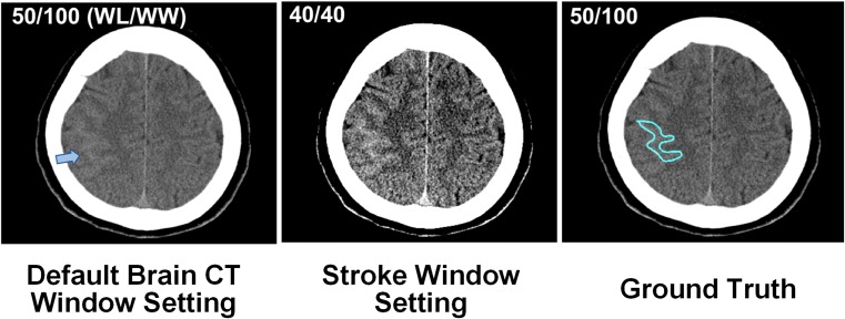
Two different approaches on CT window setting were conducted for building cascade deep learning models. The default and stroke window of a brain CT image were set to 50/100(WL/WW) and 40/40(WL/WW) respectively. Figure 3 shows an example of CT images set by two different windows. The narrower window width setting (40/40 HU) enables the emphasis of the contrast between normal and abnormal tissues, improving detection of subtle abnormality. Finally, the cascade combination of two window settings can reduce false-negative cases, which leads to an increase in sensitivity.

Fig. 3.

CT window setting on default (50/100, window level/window width) and stroke (40/40)

Diagnostic System

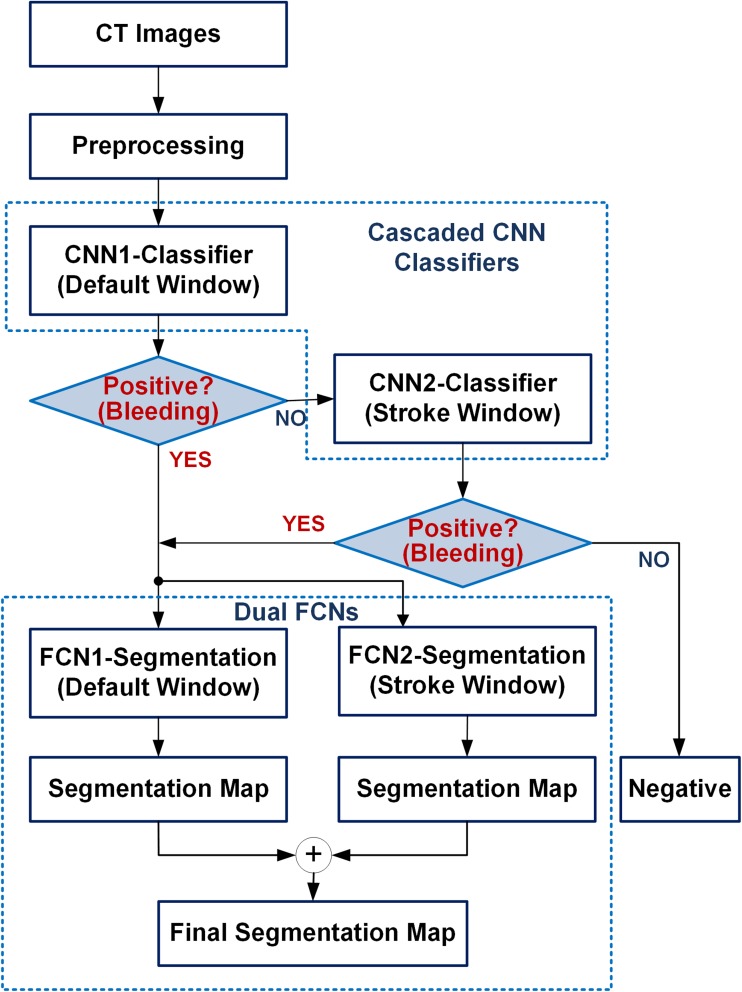
Our proposed diagnostic system consists of a cascaded CNN and dual FCN deep learning models as shown in Fig. 4. The first model identifies hemorrhage (in other words, bleeding) from the CT image. Once it is detected as bleeding, the second deep learning model predicts the subtype of hemorrhage as well as their locations. To increase sensitivity, we propose dual CT window setting approach for classification and segmentation. If it is detected as non-bleeding, the second convolutional neural network (CNN), which was trained in a narrow window width setting, reviews this case to see if it is truly negative. It helps reduce false-negative cases, resulting in an increase in sensitivity. Two FCN models trained at stroke and brain window setting were combined in parallel. Once each slice is predicted as “bleeding” by the cascaded CNN, the slice feed into each FCN model trained at different window settings. Each FCN produces a segmentation map at stroke or brain window setting. The final segmentation map is produced by merging the results from the two FCNs (logical OR). In case the label for any pixel(s) differ for the two window settings, the label predicted by the default window is assigned to it.

Fig. 4.

The flowchart of diagnostic system for detection of hemorrhage and delineation of their lesions

In computer vision, there are several popular deep CNN networks for semantic image segmentation, such as SegNet [20], U-Net [21], and FCN [22]. A large part of these is composed of encoder and decoder networks. The role of the encoder is to take input images, to extract features, and to reduce the dimensionality through the combination of convolution and pooling operations. Most of the encoders use the VGG 16 or ResNet-based CNN model. The decoder works opposite of the encoder. Instead of down-sampling the input, the decoder uses up-sampling or un-pooling with transposed convolution (deconvolution). For finer segmentation, the decoder brings some information from the encoder network. In case of SegNet, the decoder brings pooling indices to keep high frequency details in the segmentation. These kinds of the encoder-decoder networks also have been widely applied to medical applications such as lung segmentation [23], prostate segmentation [24], and myocardial segmentation in cardiac MRI [25]. U-Net is a modification from the FCN architectures with more skip connections and less parameters because of the lack of fully convolutional layers. It is slightly superior to FCN-8s on certain problems where the amount of data available is limited. Hence, it has been popular in the biomedical imaging field. However, when data available is relatively abundant FCN-8s and U-Net seems to perform similarly. FCN-8s which itself is a modification to the VGG architecture that has been widely used in other applications as well. There are more readily available pre-trained networks trained on large datasets available with the FCN-8s/VGG. This made it preferable for us to use and to do transfer learning. Probably due to this reason, not only did the FCN-8s training converge a lot faster than U-Net training for our dataset but had a slightly better performance as well.

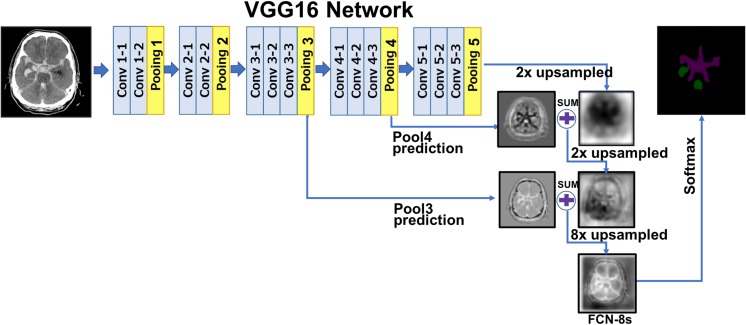
Figure 5 illustrates the FCN model which is applied to segment hemorrhage lesion. Basically, the FCN model uses VGG16 architecture as an encoder. During the five pooling steps, the input image is down-sampled up to 32 times. If up-sampling with transposed convolution by 32 is processed at the last pooling layer, it produces coarse segmentation maps (i.e., FCN-32s). To generate finer segmentation maps, FCN-8s brings high resolution feature maps from pooling layer 3 to pooling layer 5, combines them, and finally conducts 8 times of up-sampling with deconvolution operators.

Fig. 5.

Fully convolutional neural network for hemorrhagic lesion segmentation

Experiment

Training of Cascaded CNNs and Dual FCNs

First, a cascaded CNN classifier was built to identify hemorrhage by applying GoogLeNet with 22 convolutional layers, including 9 Inception modules [26]. Through fivefold cross validation, a total of 5702 patients, of which 3055 were non-bleeding and 2647 were bleeding was split into fivefold by patient cases. We first split the data based on patients’ IDs. After that, all slices from that patient was included in that cross validation fold. We employed a lot of caution regarding not mixing training and validation slices of the same patient across the folds and across repeat experiments. The cascaded CNNs were trained on a high performance computer such as NVIDIA DGX-1 with 8 Tesla V100. We trained the CNNs with two different training solvers: stochastic gradient descent (SGD) and adaptive moment estimation (ADAM). The base learning rate of weight filters was set at 0.001 and decreased by three steps in accordance with training epochs. Each CNN model was trained on CT images, which were differently preprocessed by default (50/100) and stroke (40/40) CT window settings, respectively. Trained two CNNs were combined in cascade. We also evaluated classification performance on transfer learning by initializing weights from a pre-trained model in Caffe Zoo. Through fivefold cross validation, overall accuracy in term of sensitivity and specificity was evaluated.

In order to delineate lesions of bleeding, the FCN-8s were trained on 33,391 CT slices on the DGX-1 system. We trained the FCN-8s by ADAM with a batch size of 16 and base learning rates of 10⁻⁴, and fine-tuned all layers of VGG16 using a pre-trained model. The dual FCN model, which combined two FCN-8s, was trained in the same way as building cascade CNNs. Due to a class imbalance problem, where the number of pixels occupying a bleeding lesion is much smaller than those of a normal tissue, we used dice coefficient (DC) metric to evaluate the performance of the trained model. The DC is a measure of the overlap between the segmented regions by trained networks and the ground truth. Its value of 1 means the perfect match, whereas the value of 0 means the complete mismatch between the segmentation and the ground truth. Since the Caffe deep learning framework does not implement the DC metric as default, a DC scoring module for multi-lesion segmentation was plugged into Caffe through a custom Python layer.

Results and Discussion

Binary Classification

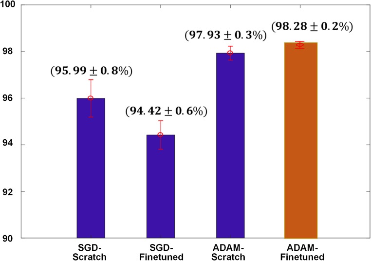
In the experiment of binary classification, we obtained the best overall accuracy of 98.28% by the CNNs trained with ADAM optimization and fine-tuned from a pre-trained model (Fig. 6). The error bar indicates the standard deviations of fivefold cross validation. A top 1 prediction for binary identification of bleeds was chosen using 0.5 as threshold. We could select high-sensitivity operating point in the receiver operating characteristic (ROC) analysis but there is a trade-off relationship between sensitivity and specificity and we will obtain poor specificity at the highest sensitivity operation point. Our goal is to improve sensitivity without decreasing specificity performance by the cascaded window setting approach for binary classification.

Fig. 6.

Results of binary classification on two different optimization schemes with and without pre-trained weights

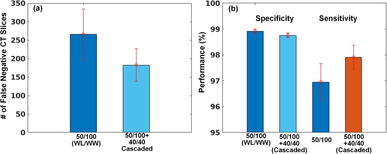
In an additional experiment, we investigated how the cascaded CT window setting helps to reduce false negatives. As you can see the left side of the bar graph in Fig. 7a, we observed that the number of predictions on false-negative cases was reduced by combining the default and stroke windows in cascade. Thus, reducing false negatives results in an increase in the sensitivity while its specificity is preserved in Fig. 7b.

Fig. 7.

Results of classification performance using the cascaded window setting. a Reducing the number of false-negative CT images and b resulting in an increase in sensitivity

Lesion Segmentation

After training the FCN-8s up to 50 epochs, we chose the best model giving the highest DC score with validation sets. Applying the best model, hemorrhagic lesions of test images were segmented, and DC scores were calculated on each lesion. Figure 8a shows the examples of segmented results on the existence of a single type of bleeding and mixture one. Both cases were well segmented compared to the ground truth in the middle with high DC scores. However, we observed that the false-negative and false-positive cases were predicted. For example, there were two ground truths on SAH (cyan colored) and SDH (green colored) in the middle of Fig. 8b but SAH lesion was well segmented with 0.84 of DC score whereas SDH lesion was not predicted (i.e., falsely negative). Both EDH and SDH lesions were well segmented in Fig. 8c but a small number of pixels representing the SAH lesion (purple colored) was falsely predicted as positives.

Fig. 8.

Examples of predicted results by FCN-8s including a well-segmented, b falsely negative, and c falsely positive case

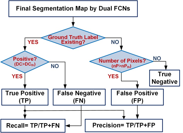
For analysis of lesion (instance) level—recall and precision, we used DC score threshold as criteria for differentiating between true positive and false negative. As shown in Fig. 9, in the slices where corresponding ground truth exists, this would be helpful to exclude small or no overlap with the predicted pixels as a true-positive prediction. This would be classified as false negative instead. When ground truth does not exist, DC score is always 0 and even a single pixel prediction would result in a false-positive prediction. We exclude instances where small number of pixels (often noise) are predicted even when no ground truth exists. These are classified as true negative instead. To clarify the process of assigning the right predictions.

Fig. 9.

A flowchart of recall and precision analysis

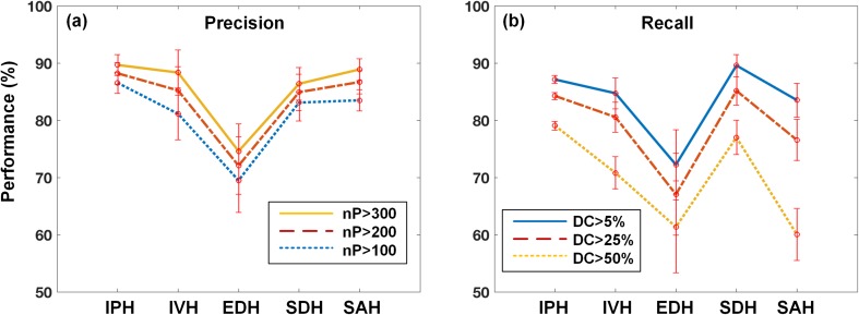
Overall precision and recall were presented on five different hemorrhagic types as shown in Fig. 10. In the precision analysis, we obtained overall accuracy ranging from 70 to 90% according to different thresholds of falsely positive segmented pixel numbers (see Fig. 9a) whereas we achieved slightly lower recall than precision at different DC threshold (see Fig. 9b). However, if we decide to set true positives at lower threshold DC, recall or sensitivity will increase.

Fig. 10.

Overall a precision and b recall according to different thresholds as falsely positive and negative decision: nP is the number of predicted pixels and DC is the dice coefficient

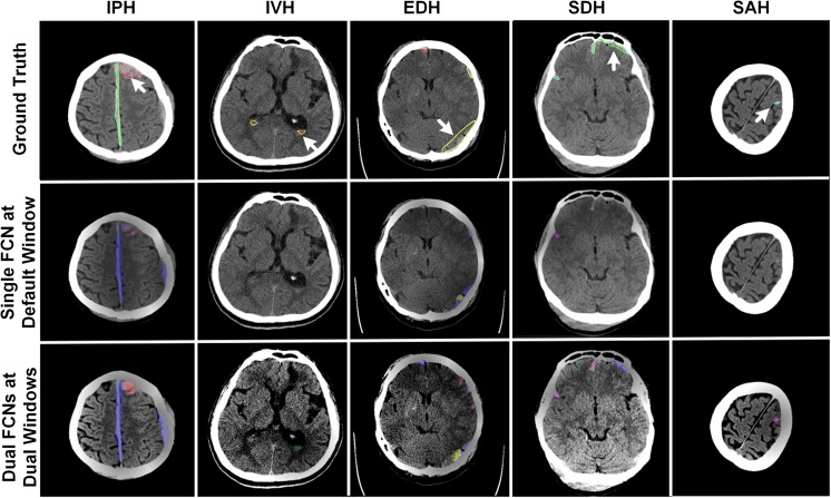
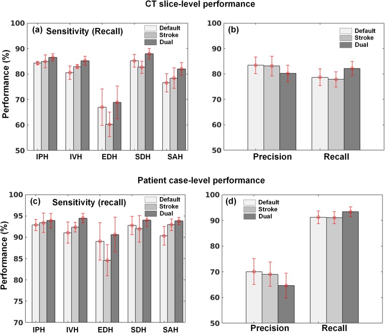
Using the dual FCN model for segmentation, the cases of falsely negative segmented lesions were reduced and some examples are shown in Fig. 11. Compared to the segmented ground truth regions, the lesions delineated by the dual FCN model (shown at the bottom row in Fig. 11) were positively predicted. Meanwhile, small numbers of pixels by a single FCN model were positively segmented or no pixels were predicted. We also observed that most of the subtle changes on CT images have been detected and segmented with our approach. Subsequently, it leads to an increase in sensitivity for detecting each type of hemorrhagic lesions in Fig. 12a, b. Compared to a single FCN model regarding precision and recall, the dual FCN model gave 82.15% recall which is an improvement of 3.44%, while precision decreased by 3.23%. We also evaluated patient-case level performance. We determined true positive if the case included at least one slice with a true positive at given decision thresholds (DC_th = .25). If not, it was regarded as false negative. In the same way, we also determined false positive if the case included at least one slice false positive at given threshold (nP_th = 200). In overall, we also obtained 2.16% improvement of sensitivity in Fig. 12c, d.

Fig. 11.

Examples of positively segmented CT images on third row using the dual FCN deep learning model, whereas they are predicted as negatives on the second row using a single FCN model trained on the default CT window setting. On the first-row images, the white arrow indicates ground truth of each hemorrhagic type

Fig. 12.

Comparison of CT-slice level (a, b) and patient case-level (c, d) performance between single (at default and stroke window) and dual FCN model at five intracranial hemorrhage and their overall precision and recall

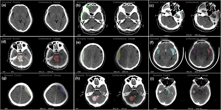
Although our diagnostic system was highly accurate in detecting hemorrhage lesion, several diagnostic errors were still found in false negative (FN) and false positive (FP). Thus, we reviewed both FN and FP cases again from a clinical and engineering perspective. In FN cases, most of them were misinterpreted as other hematomas and this can be categorized as the following: (a) a very small hematoma, which was difficult to detect due to few pixels on CT; (b) low- or iso-density of subacute and old hematomas, making it difficult to discriminate from the normal brain tissue; (c) wide-spreading hematomas of SAH, EDH, or SDH on the base of the skull which can be misinterpreted as IPH because of cross-sectional image; (d) IVH adjacent to massive IPH, which was interpreted as IPH or undefined, as a result of the distortion of normal structure of ventricle; and (e) cross-misinterpretation between EDH and SDH, due to having similar shapes in case of small hematoma (Fig. 13a–e). With regard to FP cases, most of them could be classified as the following: (f) massive hematomas of SAH in the Sylvian fissure which were misinterpreted as IPH; (g) cross-misinterpretation between EDH and SDH, like the FN case; (h) IPH adjacent to the fourth ventricle, misidentified as IVH; and (i) Partial volume effect of the skull which was misinterpreted as IPH (Fig. 13f–i).

Fig. 13.

Typical examples of false-negative (a–e) and false-positive cases (f–i): each left side is a ground truth CT image and right side is the corresponding inference result

To reduce the number of FN and FP cases, we can apply a more advanced deep learning architecture for lesion segmentation. Current FCN-8s scheme has its limitations on capturing features at multiple scales due to using one sized 3 × 3 filter. Recently dilated convolution (a.k.a. atrous convolution) enables one to enlarge the field-of-view and their pyramid combination with multiple sampling rates, and helps to represent a multi-scaled imaging object [27, 28]. It is hypothesized that filters with a large field-of-view are necessary to distinguish EDH from SDH, or widely spreading hematomas, as their lesions are occupied in a wide area of the skull (see Fig. 13e, g). The pyramid parsing module [29] could be another promising approach as it is capable of representing different sub-region, including local and global scene class. This approach will be effective in capturing massive hematomas of SAH in the Sylvian fissure as a small local lesion, which is similar to IPH, will not be misclassified (see Fig. 13f).

Conclusion

In this work, we developed our unique diagnostic system of identifying the types of hemorrhage as well as segmenting their lesions. In terms of diagnostic accuracy, there is a tradeoff between sensitivity and specificity. While conserving specificity in order to improve sensitivity, a cascade deep learning models was built by using two CNNs. In general, radiologists try to adjust contrast by setting narrower CT window width to detect subtle abnormalities. Based on this, each of the CNN and FCN was trained on the image data, preprocessed by two different CT window settings. One is a default window (50/100) and the other is a stroke window setting (40/40). By combining them, we obtained better sensitivity on the binary classification and segmentation of hemorrhagic lesions.

In our diagnostic system, identifying bleeding on a binary classifier was very crucial in the first step. We obtained the best top-1 classification accuracy of 98.28% by the CNNs trained with ADAM optimization solver and fine-tuned using a pre-trained model. With a cascade CNN model, we acquired the 97.91% of sensitivity which is about 1% improvement. In the next step of detecting hemorrhagic types and segmenting their lesions, we trained the dual FCN-8s architecture on all cases labeled as bleeding. Based on the fivefold cross validation, we obtained overall segmentation accuracy of 80.19% in precision and 82.15% in recall which is a better result than a single FCN model by 3.44%.

Compliance with Ethical Standards

This data collection was reviewed and approved by the ethics committee at Kyungpook National University Hospital and Kyungpook National University Hospital Chilgok (KNUH 2017-06-005 and KNUCH 2016-11-050).

References

- 1.Organization WH: World health statistics 2015: World Health Organization, 2015
- 2.Bluhmki E, Chamorro Á, Dávalos A, Machnig T, Sauce C, Wahlgren N, Wardlaw J, Hacke W. Stroke treatment with alteplase given 3· 0–4· 5 h after onset of acute ischaemic stroke (ECASS III): additional outcomes and subgroup analysis of a randomised controlled trial. Lancet Neurol. 2009;8:1095–1102. doi: 10.1016/S1474-4422(09)70264-9. [DOI] [PubMed] [Google Scholar]
- 3.Disorders NIoN, Group Sr-PSS Tissue plasminogen activator for acute ischemic stroke. N Engl J Med. 1995;333:1581–1588. doi: 10.1056/NEJM199512143332401. [DOI] [PubMed] [Google Scholar]
- 4.Hu T-T, Yan L, Yan P-F, Wang X, Yue G-F. Assessment of the ABC/2 method of epidural hematoma volume measurement as compared to computer-assisted planimetric analysis. Biol Res Nurs. 2016;18:5–11. doi: 10.1177/1099800415577634. [DOI] [PubMed] [Google Scholar]
- 5.Bhadauria H, Dewal M. Intracranial hemorrhage detection using spatial fuzzy c-mean and region-based active contour on brain CT imaging. SIViP. 2014;8:357–364. doi: 10.1007/s11760-012-0298-0. [DOI] [Google Scholar]
- 6.Muschelli J, Sweeney EM, Ullman NL, Vespa P, Hanley DF, Crainiceanu CM. PItcHPERFeCT: Primary intracranial hemorrhage probability estimation using random forests on CT. NeuroImage Clin. 2017;14:379–390. doi: 10.1016/j.nicl.2017.02.007. [DOI] [PMC free article] [PubMed] [Google Scholar]
- 7.Al-Ayyoub M, Alawad D, Al-Darabsah K, Aljarrah I. Automatic detection and classification of brain hemorrhages. WSEAS Trans Comput. 2013;12:395–405. [Google Scholar]
- 8.Jones N. The learning machines. Nature. 2014;505:146–148. doi: 10.1038/505146a. [DOI] [PubMed] [Google Scholar]
- 9.Patel A, Manniesing R: A convolutional neural network for intracranial hemorrhage detection in non-contrast CT. Proc. Medical Imaging 2018: Computer-Aided Diagnosis: City
- 10.Phong TD, et al.: Brain Hemorrhage Diagnosis by Using Deep Learning. Proc. Proceedings of the 2017 International Conference on Machine Learning and Soft Computing: City
- 11.Arbabshirani MR, Fornwalt BK, Mongelluzzo GJ, Suever JD, Geise BD, Patel AA, Moore GJ. Advanced machine learning in action: identification of intracranial hemorrhage on computed tomography scans of the head with clinical workflow integration. npj Digit Med. 2018;1:9. doi: 10.1038/s41746-017-0015-z. [DOI] [PMC free article] [PubMed] [Google Scholar]
- 12.Jnawali K, Arbabshirani MR, Rao N, Patel AA: Deep 3D convolution neural network for CT brain hemorrhage classification. Proc. Medical Imaging 2018: Computer-Aided Diagnosis: City
- 13.Grewal M, Srivastava MM, Kumar P, Varadarajan S: RADnet: Radiologist level accuracy using deep learning for hemorrhage detection in CT scans. Proc. Biomedical Imaging (ISBI 2018), 2018 IEEE 15th International Symposium on: City
- 14.Titano JJ, et al. Automated deep-neural-network surveillance of cranial images for acute neurologic events. Nat Med. 2018;24:1337–1341. doi: 10.1038/s41591-018-0147-y. [DOI] [PubMed] [Google Scholar]
- 15.Chilamkurthy S, et al.: Development and Validation of Deep Learning Algorithms for Detection of Critical Findings in Head CT Scans, 2018 [DOI] [PubMed]
- 16.Chang P, et al.: Hybrid 3D/2D Convolutional Neural Network for Hemorrhage Evaluation on Head CT39:1609–1616, 2018 [DOI] [PMC free article] [PubMed]
- 17.Lev MH, Farkas J, Gemmete JJ, Hossain ST, Hunter GJ, Koroshetz WJ, Gonzalez RG. Acute stroke: improved nonenhanced CT detection—benefits of soft-copy interpretation by using variable window width and center level settings. Radiology. 1999;213:150–155. doi: 10.1148/radiology.213.1.r99oc10150. [DOI] [PubMed] [Google Scholar]
- 18.Turner P, Holdsworth G. CT stroke window settings: an unfortunate misleading misnomer? Br J Radiol. 2011;84:1061–1066. doi: 10.1259/bjr/99730184. [DOI] [PMC free article] [PubMed] [Google Scholar]
- 19.Lee H, et al. Pixel-level deep segmentation: artificial intelligence quantifies muscle on computed tomography for body morphometric analysis. J Digit Imaging. 2017;30:487–498. doi: 10.1007/s10278-017-9988-z. [DOI] [PMC free article] [PubMed] [Google Scholar]
- 20.Badrinarayanan V, Kendall A, Cipolla R. Segnet: A deep convolutional encoder-decoder architecture for image segmentation. IEEE Trans Pattern Anal Mach Intell. 2017;39:2481–2495. doi: 10.1109/TPAMI.2016.2644615. [DOI] [PubMed] [Google Scholar]
- 21.Ronneberger O, Fischer P, Brox T: U-net: Convolutional networks for biomedical image segmentation. Proc. International Conference on Medical image computing and computer-assisted intervention: City
- 22.Long J, Shelhamer E, Darrell T: Fully convolutional networks for semantic segmentation. Proc. Proceedings of the IEEE conference on computer vision and pattern recognition: City [DOI] [PubMed]
- 23.Kalinovsky A, Kovalev V. Lung image segmentation using deep learning methods and convolutional neural networks. 2016. [Google Scholar]
- 24.Milletari F, Navab N, Ahmadi S-A: V-net: Fully convolutional neural networks for volumetric medical image segmentation. Proc. 3D Vision (3DV), 2016 Fourth International Conference on: City
- 25.Curiale AH, Colavecchia FD, Kaluza P, Isoardi RA, Mato G: Automatic Myocardial Segmentation by Using A Deep Learning Network in Cardiac MRI. arXiv preprint arXiv:170807452, 2017
- 26.Szegedy C, et al.: Going deeper with convolutions: City
- 27.Chen L-C, Papandreou G, Kokkinos I, Murphy K, Yuille AL. Deeplab: Semantic image segmentation with deep convolutional nets, atrous convolution, and fully connected crfs. IEEE Trans Pattern Anal Mach Intell. 2018;40:834–848. doi: 10.1109/TPAMI.2017.2699184. [DOI] [PubMed] [Google Scholar]
- 28.Chen L-C, Papandreou G, Schroff F, Adam H: Rethinking atrous convolution for semantic image segmentation. arXiv preprint arXiv:170605587, 2017
- 29.Zhao H, Shi J, Qi X, Wang X, Jia J: Pyramid scene parsing network. Proc. IEEE Conf on Computer Vision and Pattern Recognition (CVPR): City