Deep Learning Models Unveiled Functional Difference between Cortical Gyri and Sulci

Abstract

It is largely unknown whether there is functional role difference between cortical gyral and sulcal regions. Recent advancements in neuroimaging studies demonstrate clear difference of structural connection profiles in gyral and sulcal areas, suggesting possible functional role difference in these convex and concave cortical regions. To explore and confirm such possible functional difference, we design and apply a powerful deep learning model of convolutional neural networks (CNN) that has been proven to be superior in learning discriminative and meaningful patterns on fMRI. By using the CNN model, gyral and sulcal fMRI signals are learned and predicted, and the prediction performance is adopted to demonstrate the functional difference between gyri and sulci. By using the Human Connectome Project (HCP) fMRI data and macaque brain fMRI data, an average of 83% and 90% classification accuracy has been achieved to separate gyral/sulcal HCP task fMRI signals at the population and individual subject level respectively; 81% and 86% classification accuracy for resting state fMRI signals at the group and individual subject level respectively. In addition, 78% classification accuracy has been achieved to separate gyral/sulcal resting state fMRI signals in macaque brains. Importantly, further analysis reveals that the discriminative features that are learned by CNNs to differentiate gyral/sulcal fMRI signals can be meaningfully interpreted, thus unveiling the fundamental functional difference between cortical gyri and sulci. That is, gyri are more global functional integration centers with simpler lower frequency signal components, while sulci are more local processing units with more complex higher frequency signal components.

I. Introduction

The cerebral cortex is a continuous 2D sheet of interleaving convex gyri and concave sulci. Modern neuroimaging techniques such as magnetic resonance imaging (MRI) allow a clear delineation and differentiation of the different shape and morphology patterns of gyri and sulci, e.g., cortical segmentation of gyri/sulci based on structural MRI images in the past few decades [1–9]. However, anatomical differentiation and segmentation of gyral and sulcal regions does not tell much information about the potential functional role difference of gyri and sulci. In the neuroscience literature, neuroscientific communities from sundry disciplines have proposed many hypotheses for the mechanisms behind gyrification, for example, differential laminar growth [10, 11], genetic regulation [12, 13] and axonal tension or pulling [9, 14]. But it has been still rarely asked whether there are functional role differences between gyral and sulcal regions or not, and thus it has been traditionally assumed that there is no functional role difference between cortical gyri and sulci [15–17].

Thanks to advanced neuroimaging techniques, such as diffusion tensor imaging (DTI) and functional magnetic resonance imaging (fMRI), we can observe the structural and functional profiles of cortical gyri and sulci in unprecedented details in vivo. A growing number of studies show differences in gyral and sulcal regions, including structural and functional connectivity patterns [7,18–21]. For example, neuroimaging and bioimaging studies revealed that DTI-derived streamline fiber terminations mainly concentrate on gyri [21, 22]. Other studies have also made efforts to study the difference between gyri and sulci from the functional perspective [18, 20, 23, 24]. In [18], author demonstrated that the functional connectivity is strong among gyri, weak among sulci, and moderate between gyri and sulci. These results suggest that gyri are functional connection centers that exchange information among remote structurally-connected gyri and neighboring sulci, while sulci communicate directly with their neighboring gyri and indirectly with other cortical regions through gyri. In [23], Jiang found that the identified THFRs (task-based heterogeneous functional regions) locate significantly more on gyral regions than on sulcal regions, suggesting gyri may focus more on the tasks or natural stimulus. In [20], Liu pointed out that gyri are more functionally integrated, while sulci are more functionally segregated. Above-mentioned findings suggest that functional difference between gyri and sulci indeed exist. In addition, frequency domain is an important research field to study and understand the functional characteristics of the brains [25–27]. For example, in [25], Stephan reported that committing to the different frequency galvanic vestibular stimulation (GVS) with alternating currents, the activation areas on the brain cortical surfaces are different, i.e., different brain regions may respond to different frequency stimuli. To our best knowledge, no research result has directly focused on exploring the functional characteristics of gyri and sulci in frequency domain. In conclusion, previous studies suggest the potential for functional difference between gyri and sulci. However, due to the complexity and variability of the structure and function of the cerebral cortex [15, 28–30], the functional role difference between cortical gyral and sulcal regions is largely unknown, nor the mechanisms that characterize and underlie such differences are understood.

In order to address the above mentioned complexity and variability of the structure and function of the cerebral cortex and to discover the intrinsic functional difference between gyri and sulci based on the fMRI signals, we need a powerful computing algorithm which has both computing power and learning power to handle the hundreds of thousands of fMRI signals in an individual brain. Recently, deep learning methods such as convolutional neural network (CNN) have attracted increasing attention in the field of machine learning and data mining [31–37], and they have been proven to be very powerful for learning discriminative and meaningful features from raw data. In particular, CNN has been applied to image classification and text classification problems, and promising results have been achieved [38–45]. Recently, deep learning algorithms have been also applied on the fMRI studies [46–49]. For example, deep learning algorithms have been adopted to differentiate brain network maps derived from fMRI scans [50], better results are achieved compared with traditional methods. Another example is that we recently developed a Deep Convolutional Auto-Encoder (DCAE) [46] to model task-based fMRI (tfMRI) data by taking the advantages of both data-driven approach and CNN’s hierarchical feature abstraction ability for learning mid-level and high-level features from complex tfMRI time series in an unsupervised manner. These successes inspired us to model and analyze fMRI time series data of gyri/sulci by one dimensional CNNs and to learn discriminative features that can potentially differentiate cortical gyri and sulci from a functional perspective. Thus, in this study, we propose a new strategy by adopting one dimensional CNN model to differentiate temporal fMRI signals on gyri and sulci. Our hypothesis is that fMRI signals of gyri and sulci have fundamental differences. These differences can be represented through fMRI signals and be well characterized and classified by the proposed CNN model. Importantly, the CNN model can also learn the discriminative features that can be used to characterize and interpret such functional role differences between gyri and sulci.

The carefully designed CNN models are then applied on multiple fMRI datasets, including both task-based fMRI and resting state fMRI of human and monkey brains, and our experimental results consistently showed that gyral and sulcal fMRI signals can be differentiated and accurately classified across species (both macaque and human), across tasks and resting state situations (7 HCP tasks and resting state), and across populations (both individual level and group level). These overwhelming results confirmed the true functional differences of cortical gyri and sulci. Our further interpretations of the learned features by CNN models and their frequency distributions in gyri/sulci suggest that low frequency and high frequency features play different roles to differentiate gyri and sulci, and that gyral regions might have more basic and global functions while sulcal regions might have more complex and local functions. In general, our works revealed the fundamental functional role differences of gyri and sulci, and provide a new window to study the complex functions of the cerebral cortex.

II. Materials and Methods

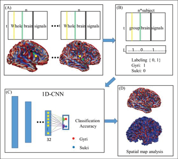
The framework of 1D CNN to classify gyral and sulcal fMRI signals includes four major steps (marked as (A)-(D) in Fig. 1). First, we extract gyral and sulcal fMRI signals separately from the whole brain. We annotate each extracted fMRI signal with either gyrus or sulcus label by checking the label of the corresponding vertex on the cortical surface. Assume the landmark j is a vertex on the brain, and k_j is the candidate location in its morphological neighborhood. The maximum principal curvature of k_j is represented by P, if P≥0, j belongs to gyri, and if P<0, j belongs to sulci. For more details, please refer to [51]. Second, we aggregate gyral or sulcal fMRI signals from all the studied subjects together and then divide the aggregated signals into training and testing datasets, respectively. Third, we use the 1D CNNs to train the model and classify the gyral and sulcal signals. The last step is result presentation and analysis, in which the learned features by CNNs are explained and interpreted within a neuroscientifically meaningful context.

Fig 1.

The pipeline of the proposed computational framework of using 1D CNNs to classify gyral/sulcal fMRI signals. (a) Extract gyral and sulcal signals across the whole brain. Here n is the total number of gyral and sulcal vertices in the whole brain, and t is the time points according to the specific task. Color lines in the matrix represent the BOLD time-series corresponding with the same color vertex shown on the cortical surface. (b) Aggregate all the matrices into a big one and label each vertex with label 1 (gyrus) or 0 (sulcus). (c) The 1D CNN is applied to train the model and classify the gyral/sulcal fMRI signals. (d) Further analysis and interpretation based on the features learned by 1D CNN.

A. Data acquisition and preprocessing

The Human fMRI data

In this study, the high-resolution task-based fMRI (tfMRI)/resting state fMRI (rsfMRI) from the HCP datasets [16, 52, 53] are used. In the Q1 release of HCP fMRI dataset, 77 participants are scanned. Specifically, 58 are female and 19 are male, 3 are between the ages of 22–25, 27 are between the ages of 26–30, and 47 are between the ages of 31–35. In the publicly released dataset, 60 subjects are available and used in this paper. For individual level study, each subject will be studied separately. For the group level study, 10 subjects will be treated as one group, thus we have 6 groups in total. So our experiments are based on the seven tasks and one resting state fMRI data of 60 subjects. The acquisition parameters of tfMRI data are as follows: 90 × 104 matrix, 220 mm FOV, 72 slices, TR = 0.72 s, TE = 33.1 ms, flip angle = 52, BW= 2290 Hz/Px, in-plane FOV = 208 × 180 mm, 2.0 mm isotropic voxels. The tfMRI data consist of seven task paradigms, including emotion, gambling, language, motor, relational, social, and working memory (WM) tasks. The HCP tasks were designed to identify core functional nodes across a wide range of the cerebral cortex. For tfMRI images, the preprocessing pipelines included skull removal, motion correction, slice time correction, spatial smoothing. All of these steps are implemented by FSL FEAT, and more details please refer to [53]. For the rsfMRI data, the pre-processing steps include skull removal, motion correction, slice time correction, spatial smoothing. More detailed rsfMRI preprocessing steps can be referred to the literature report [52, 54]. In this paper, the Q1-release HCP dataset (60 subjects) is used to develop and evaluate our 1D CNN models.

Monkey fMRI data

The macaque subjects were members of a colony in the Yerkes National Primate Research Center (YNPRC) at Emory University in Atlanta, Georgia. All imaging studies were approved by the IACUC of Emory University. Six 6-month-old macaques with multimodal T1-weighted MRI, DTI and rsfMRI scans were used as a testbed in this study. The main imaging parameters are as follows. For T1-weighted MRI, repetition time/inversion time/echo time is 3000/950/3.31 msec, flip angle = 8°, matrix is 192×192×128, and resolution is 0.6×0.6×0.6 mm³ with 6 averages. For DTI, b value is 1000 sec/mm², 62 directions of diffusion-weighting gradients, repetition time (TR)/echo time (TE) is 5000/90 msec, FOV (field of view) is 83.2×83.2 mm², matrix size is 64×64×43 covering the whole brain, and resolution is 1.3×1.3×1.3 mm³. Ten runs of DTI scans were performed for each subject. One image without diffusion weighting (b=0 sec/mm²) was acquired with matching imaging parameters for each average of diffusion-weighted images, DTI data is used to generate cortical surface. For rsfMRI, TR/TE is 2060/25 msec, matrix is 85×104×65, resolution is 1×1×1 mm³, and there are 400 time points.

B. Extract gyral and sulcal fMRI signals and prepare the training/testing samples

In order to separate the gyral/sulcal fMRI signals in an individual brain, a crucial step is to differentiate the neuroanatomic gyral/sulcal areas and then to extract the corresponding fMRI signals, which is shown in Fig.1A. Here, three steps are included in Fig.1A. First, we reconstruct the cortical surface of each human brain based on the individual’s DTI data (the fMRI and DTI sequences are both EPI (echo planar imaging) sequences, and thus their distortions tend to be similar and the misalignment between DTI and fMRI images is much less than that between T1 and fMRI images [57]. Co-registration between DTI and fMRI data can be robustly performed using FSL FLIRT). Second, we use linear registration algorithm to register the individual fMRI data to its own DTI space, and we want to emphasize that both the registered fMRI and cortical surface are under the subject’s individual DTI space. The reason to register fMRI onto DTI space is that we want to keep its original anatomical and structure information. Third, we assign the fMRI temporal signals to each vertex on the cortical surface. We will match each vertex on the cortical surface with its nearest fMRI voxel from registered fMRI data and assign the signal of that fMRI voxel to that cortical surface vertex. In this way, all the vertices on the cortical surface will have their own fMRI signals. After the standard fMRI signal pre-processing for each subject, the next step is to aggregate all the fMRI signals together as shown in Fig.1B and then to divide them into training samples and testing samples, respectively. For the high-quality HCP dataset, not all the vertices on the surface are used for training and testing. About 30% vertices with the highest maximum principal curvature values are labelled as gyri and another 30% vertices with the lowest curvature values are labelled as sulci. So in total, 60% vertices from each subject will be used. The vertices with values in the middle will not be used and not be labelled in this paper to avoid ambiguity (for more details about the middle vertices, please see the supplemental materials). Based on the selected vertices, 80% of those labelled gyral/sulcal vertices from each subject are used as training data, and the rest 20% are used as testing data. Training data is used to train the model and testing data is used to examine the performance of the learned model. The assumption that we make for the task fMRI experiment in a group level is that fMRI signals in different brains have relatively good consistency under the same task performance. The assumption that we make for the rsfMRI experiment in a group level is that although we know that the functional signals could be quite different from different subjects under the resting state, the differences between fMRI signals of gyri/sulci should exist and be quite consistent. In addition, deep CNN model is more powerful and effective based on larger dataset, e.g., more training samples will contribute to better chance to discover consistent and common differences between gyral and sulcal fMRI signals. Meanwhile, for each individual, we expect that greater classification accuracy can be achieved.

C. Structure of 1D CNN model

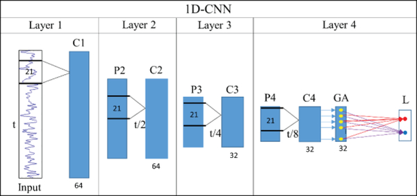
In this section, A CNN model is usually composed of alternate convolutional and pooling layers to extract hierarchical features to represent the original inputs, subsequently with several fully connected layers followed to perform classification. In this paper, we specifically deal with 1D temporal fMRI time series signals using CNN, as shown in Fig 1c. Inspired by previous deep CNN studies [46], as shown in Fig.2, we designed a deep 1D CNN architecture to differentiate gyral/sulcal fMRI signals to explore the intrinsic differences between gyri and sulci from a functional perspective. For the input layer, the fMRI signals are obtained by the method we mentioned above with two labels to represent gyri and sulci. Based on the different subjects and different tasks or resting state fMRI data, the dimension of the inputs could be varying, however the structure of the inputs is the same, which is N*T, where N is the total number of used vertices from a group number of subjects, and T is the time points of current fMRI data. For the network architecture, as shown in Fig.2, the convolutional layer (C), pooling layer (P), and global average layer (GA) are included accordingly. In total, we use 64 filters in the first and second C layers, and employ 32 filters in the third and fourth C layers. 32 neurons in the GA layers and 2 neurons in the output layer. Specifically, the 2 neurons in the output layer represent the gyrus and sulcus labels, respectively, denoted as the red and blue dots in Fig.2. For the parameter settings, we set the length of the filter fixed as 21 across the layers. Similar to the traditional CNN structure, a filter is only connected with certain local area from the previous input data. In this paper, the filter size is defined as a window with the range of 21 time points. So using one fMRI time series from the input data as an example, a small part of this input fMRI signal $I_{t_l,t_{l+20}}$ within the window (as shown in the Fig.2 layer 1) will be sent to the filters in the first layer, where l represents one time point from fMRI signals. Then, the window will change a little by moving one time point down, the new input is $I_{t_{l+1},t_{l+21}}$, then this new local information will be sent to the filters again, which is repeated until the window reaches t_L where L is the length of the fMRI time series. For the next layer, filters do not directly reach to the input fMRI time series and they are connected with the previous layer, and inputs are the output from the previous layer. The structure is shown in the Fig.2.

Fig 2.

The structure of the 1D CNN model (4 convolutional layers as an example). C means convolutional layer, P is short for max pooling, GA means global average layer, and L is the output layer which contains 2 labels (gyri/sulci). The length of filter is fixed as 21.

Epoch is generally defined as “one pass over the entire dataset”. After one epoch is trained, another epoch will start by doing what we mentioned above again, repeat this until training process is stopped. In this paper, epoch is set to 30 and then our approach will check whether the loss function has converged to decide whether training process is complete. So, here 30 epochs mean, during training, the whole input data are trained one epoch after one epoch to achieve classification performance and repeated for 30 epochs. After each epoch, the model of current stage will be saved, that is, all the parameters and filters will be saved, the logging and periodic evaluation of current epoch will be recorded too. So, by picking up the best epoch, we can obtain the corresponding model and then obtain all the parameters, filters and features’ information from that model. So, after going through all 30 epochs, if the loss function is already converged, we will use model evaluation to examine the models and the best one will be picked up. Then we use the best model to examine the testing data. If not, we will keep training more epochs. In this paper, experiments are well trained within 30 epochs.

In this work, the “Relu” activation function is used due to at least two reasons: one major benefit is the reduced likelihood of the gradient to vanish and it is faster than many other activation functions. Another one is that ReLUs is sparse, and sparse representations seem to be more beneficial than dense representations, because a very dense distributed representation can be difficult to learn and overwhelm true dependencies, which will have an undue influence on the result. Specifically, in this paper, we would like to know the true differences between gyral signals and sulcal signals, thus we need to remove the noise, distant dependencies and etc. For those input fMRI signals, the dense representations will include more nuisance dependencies, and these nuisance dependencies could overwhelm true dependencies. For the loss function, we used “categorical_crossentropy” function from Keras tool.

In order to investigate the performance of classification from input to output and understand the progress of deep learning layer by layer, we design a pipeline to explore the performance of each layer from the back to the front. By preforming this process, details of the whole CNN structure are better understood. Here, we take Fig.2 as an example to show how the pipeline works to achieve the objective. From Fig.2 we can see that the whole structure is divided into four layers, each layer containing one convolutional layer. Among these 4 layers, layer 4 is a special one, since it already has the global average layer and output layer, and the performance of classification of this layer can be easily obtained. Compared with layer 4, other three layers do not have GA and L. So the performance is not directly clear. However, since the model is already trained, in order to assess the performance of layer 3, we keep the model fixed and just delete the layer inside layer 4 and then add GA and L connected to the C3. Here, we want to mention that the output dimension of each of convolutional layer is different, but there is no mismatch in dimension for GA and L layer in our model. Because we design our GA and L layer based on their previous layer. So if the previous layer changed, GA layer will be changed automatically to fit for the whole model. Similarly, to assess the performance of layer 2, we delete layer 3 and 4, and add GA and L connected to the C2. In this way, we let the input to go through the new structure, and thus the classification results of the exact layer can be unveiled.

D. Classification performance analysis and visualization

To understand the CNN’s output layer L, we need to carefully examine the CNN model that is trained already. If the input is n*t fMRI signals from one subject, then the output will be a matrix of n*2, meaning that for each vertex, 2 values can be obtained and compared. These two values are corresponding to the labels from layer L, and the label with the larger value will be given to the vertex. After predicting the labels for each vertex’s fMRI signal, the labels can be mapped back onto the cortical surface, in that the output of the CNN’s last layer and the input of the CNN have vertex-to-vertex correspondence. The distribution pattern of the spatial map will informatively show the CNN’s classification accuracy, and thus the accurate classification and misclassification can be understood and interpreted in a meaningful context of neuroanatomic regions.

To unveil the progress of classification layer by layer, we need to explore the features from each convolutional layer, which is presented by C1-C4 in this paper. To our best knowledge, the classification capability of different layers could be quite different and they are decided mainly by the filters. Thus, filters are the units that we will pay special attention to. Using layer 4 from Fig.2 as an example, within this convolutional layer, 32 filters are contained. In each filter, 32 features are recorded due to that the last convolutional layer in layer 3 has 32 filters. In addition, GA is global average layer based on the previous convolutional layer. GA and L layers are fully connected layer, GA has the same number of nodes as the filter numbers from previous convolutional layer, and L has two nodes, as they are designed as gyri and sulci in this work. Thus, for each node in the GA layer, it represents a filter from the previous layer and it has two connections to the two nodes in the L layer, respectively. Weight value of each connection represents the possibility of this GA node belonging to, maximum weight value among two values was picked up and the corresponding connection will represent the label of that GA node, either gyri or sulci. For example, if the connection between GA node and L gyri node is picked up, it means the corresponding filter is gyri filter. In this way, filters can be labelled as well as vertices.

So three types of analyses are performed for filters and layers. The first one is the characteristics of features from gyral/sulcal filters, by directly extracting features from gyral filters and sulcal filters. Feature here is defined as the pattern of the weights we obtained from the filter. This will provide us with intuitive observations about the differences between gyral features and sulcal features. The second analysis method is frequency analysis by studying the frequency distribution of those features. The frequency domain of features can be converted by its original temporal signals by applying fast Fourier transform (FFT), and then a vector will be used to present its frequency and magnitude maps. The third analysis is the Pearson correlation among all the features within one filter, and we define the average Pearson correlation of filter i as C_i. So the equation of obtaining C_i is shown as follows:

$$C_i=({\sum }_{x,y=\mathrm{1..}n,x\ne y}\frac{cov(x,y)}{{\sigma }_x{\sigma }_y})/(n(n-1))$$ (1)

where x and y are the features, and n is the number of the features in the filter i. Then average Pearson correlation of one layer can be easily calculated by averaging all the Pearson correlations of filters within this layer.

III. Results

A. Gyral and sulcal fMRI signals are largely different at the population level

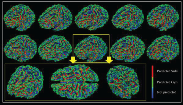
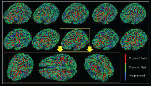
When applying the 1D CNN algorithm on the HCP 7 tasks dataset, for each task, we group 10 subjects’ fMRI data as the testbed to train the model and test the classification performance. Typically, 10 subjects’ tfMRI data contain around 1,000,000 tfMRI time series in total (about 100,000 for each). After 30% vertices with the highest curvature values and about 30% vertices with the lowest curvature values are picked up, so there are around 600,000 tfMRI time series in total. Among those 600,000 signals, 80% tfMRI time series are used as training samples and the rest are used for testing. Training samples are used to train the model and testing samples are used to examine the performance of the model on the new data (no overlap between training and testing samples). In order to intuitively present the testing classification results for each task, we showed them in Table 1. After we identify the best model and its parameters and weights, all the fMRI signals of used vertices from corresponding subject will be picked up to generate an input. We put this input into the best model and the outputs from the model will be the labels it predicted for each vertex, and then predicted labels will be shown on the cortical surface for each vertex as we mentioned in the method part D. Then the classification performance for the corresponding subject can be obtained and visualized like the examples shown in Fig.3. According to the Table 1, the testing classification accuracies are as high as nearly 80% in the testing, meaning that about 80% of vertices from gyri and sulci can be differentiated correctly. In addition, the average dice scores for gyri and sulci from task EMOTION are recorded accordingly, and they are 0.74 and 0.70, respectively. To show the performance of classification results more intuitively, we map the labels of vertices we obtained back onto the cortical surface individually. In this way, for each task, every individual has a spatial map to visually represent the classification performance. We represent 10 subjects from task EMOTION as an example in Fig.3. Other six tasks are shown in the supplemental materials (Supplemental Figures 1–6). From Fig.3, the green vertices are predicted as gyri by the CNN model we trained and the red vertices are predicted as sulci. We can clearly see from Fig.3 that misclassification occurred in some locations, for example, some red vertices can be found on the gyri and some green vertices are detected on the sulci, which are the misclassified vertices, but the majority of the classified gyral/sulcal areas are accurate and clear, especially for some local areas, like the central sulcus, precentral sulcus, inferior frontal sulcus and superior temporal sulcus. Thus, we conclude that 1D CNN model did successfully differentiate between gyral and sulcal fMRI signals.

Table 1.

Testing classification accuracy of each task at the group level.

Task	Classification accuracy	Task	Classification accuracy
EMOTION	83.3%	GAMBLING	84.4%
LANGUAGE	83.3%	MOTOR	84.6%
RELATIONAL	86.4%	SOCIAL	86.8%
WM	82.3%

Fig 3.

The classification performance of 10 subjects in task EMOTION. Each vertex on the surface is given a predicted label. Green vertices are predicted as gyri, red vertices are predicted as sulci, and blues ones are vertices that not used. Zoom-in figures are used to show the performance of one case in 3 different directions.

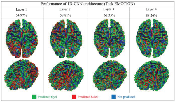
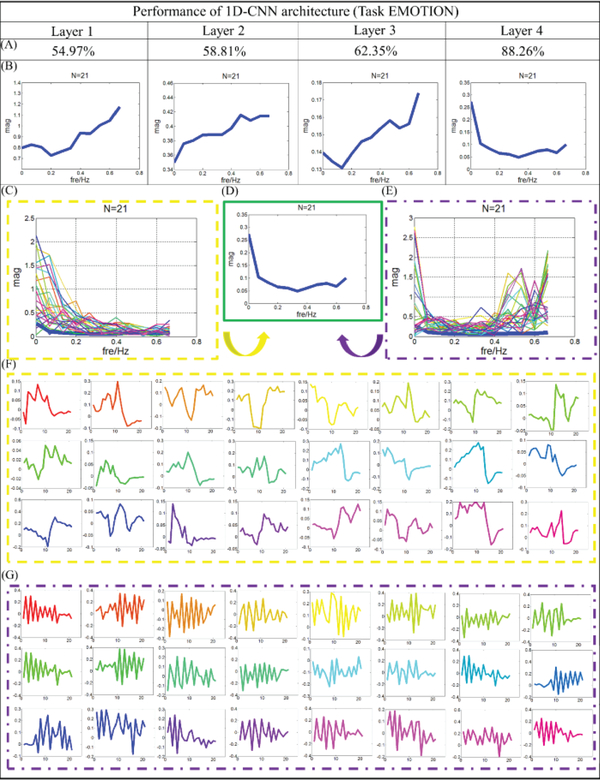
In addition to presenting the classification performance of the output layer of the CNN model, we further investigated and interpreted the 1D CNN structure and explored why it achieved such high classification performance. In particular, we are interested in how each layer of the CNN model performs and contributes to classification accuracy. As mentioned in the method section, we use multiple layers to represent the neural network architecture of the 1D CNN. By adopting the architecture analysis algorithm designed in the method part, performance of each layer is observed and analyzed. Fig.4 shows an example of EMOTION task from one randomly selected subject. Similar results for other 6 tasks are shown in the supplemental materials (Supplemental Figure 7). On this subject, the testing classification accuracy of layer 1 to 4 are 54.97%, 58.81%, 62.35% and 88.26%, respectively. As shown in Fig.4, we can clearly observe that from layer 1 to 3, the performance of the classification is not very good and not very consistent neither. For instance, gyral and sulcal regions cannot be differentiated in large areas across the whole brain, especially for the frontal lobe and occipital lobe. Then, when the layer reaches to 4, the testing classification accuracy raises to about 88% and most cortical areas can be classified correctly. Thus, we can see that the differences between gyral and sulcal fMRI signals truly exist, however, they are buried in the deeper layers of the CNN architecture and thus are difficult to be captured if using traditional shallow data mining and machine learning algorithms, such as independent component analysis and sparse dictionary learning. Using the previous study [20] as an example, sparse coding and online dictionary learning method is used to differentiate the difference between the gyri and sulci signals. Due to that it is hard to measure the signals directly, they use the dictionary learning to learn the dictionary atoms of gyri/sulci signals separately and then analyze the functional connectivity among those atoms. On average, the functional connectivity among gyri atom-gyri atom, gyri atom-sulci atom and sulci atom-sulci atom connection patterns account for a percentage of 41.2%, 36.4% and 22.4%, respectively. However, restricted by the method, they cannot map the feature to effectively and efficiently classify real gyri/sulci vertices. Instead, they only focus on the correlation of those gyri atoms and sulci atoms learned from dictionary learning method. Thus, there is no discriminative signal pattern and classification performance reported in the paper. That is the reason that we designed and employed 1D CNN model in this paper. Fortunately, the designed deep learning method 1D CNN architecture can effectively reveal such deeply buried differences. We used the same 1D CNN architecture for the different 6 tasks and all of them can achieve quite similar promising results shown in Table 1 and Supplemental Figure 7.

Fig 4.

The classification performances of 4 convolutional layers in task EMOTION at a group level. Each vertex is given a predicted label. The spatial maps of 2 different views are used to show the classification performance of each layer. Classification accuracies are recorded, respectively. Green vertices are predicted as gyri, red vertices are predicted as sulci and blues ones are vertices that not used.

In addition to its superior classification performance, CNN is also powerful in extracting meaningful features during the model training process. Thus, the investigation of the learned filters in each layer of the 1D CNN model can potentially offer a window to understand how CNN discriminate the gyral and sulcal fMRI signals. In order to do this, we pull out the features from each convolutional layer and conduct statistical analysis on the filters layer by layer, and present the results of task EMOTION in Fig.5. The results of other six tasks are shown in the supplemental materials (Supplemental Figure 8–13). In order to test the robustness of our method, all available Q1-release subjects are divided equally into 6 groups to repeat the experiment at group level, and quite consistent classification performances are shown in the supplemental materials (Supplemental Table 1).

Fig 5.

Filter feature analysis for task EMOTION. (A) Classification performance from layer 1 to 4. (B) The distribution of frequency for filter features in average level from layer 1 to 4. (C) The distribution of frequency for features from gyral filters. N is the length of the features. The distribution of frequency for the last layer is provided using bold blue line. (D) Distribution of frequency for the last layer. (E) The distribution of frequency for features from sulcal filters. N is the length of the features. The distribution of frequency for the last layer is provided using bold blue line. (F) Original features which are corresponding to (C), and the correspondence is presented by color. (G) Original features which are corresponding to (E), and the correspondence is presented by color.

As shown in Fig.5, two major aspects are explored to represent the progresses of classifying the gyral/sulcal fMRI signals through different layers. First, according to the frequency analysis, the average distribution of frequencies for all the filters in one layer is summarized and presented in Fig.5B. From layer 1 to 3, the distribution of frequency domain is more inclined to high frequency and the higher frequency exhibits the largest magnitudes, like the frequency range of 0.4–0.7 HZ. However, the classification accuracies of those layers are relatively low. When the layer reaches 4, the distribution of frequency domain is quite different from the first three layers. That is, the lower frequency range has the largest magnitudes, and in the meanwhile, the higher frequency keeps relatively high magnitudes and the middle frequency exhibits the lowest magnitudes. In this way, a good classification accuracy (88.26% from Fig. 5) is achieved from the same layer (layer 4). Interestingly, this frequency pattern is observed from all other six tasks and good classification accuracies are all achieved from the corresponding layer. Thus, we infer that certain distribution of frequency will represent certain pattern of features and those features will have the ability to differentiate the gyri/sulci. To elucidate the relationship between the distribution of frequency and classification accuracy, we went through all of the filters and features in each layer and present typical patterns for the last layer, as shown in Fig.5C. Two typical frequency patterns of the filter features are observed in the last layer: one has low frequency as shown in Fig. 5C, and another is quite high and the pattern is presented in Fig.5E. Their original features are extracted and presented in Fig.5F and Fig.5G, respectively. In contrast with the last layer, the pattern with low frequency is not discovered in the first three layers, hence both patterns are indispensable to our classification, meaning they both contribute to the good classification performance. It is worth noting that in the Fig. 5, features in the yellow frame represent the pattern from gyral filter, while features in the purple frame represent the pattern from sulcal filter. It is clear that features with lower frequency are observed in the gyral filters, but much higher frequency features are identified in the sulcal filters. In addition, the average Pearson correlation of features in each filter is analyzed using the methods shown in the equation (1). In the last layer, the average correlation of features in gyral filter is about 0.42, standard deviation is 0.03, but the average correlation is about 0.35 in the sulci filters and standard deviation is 0.035. That means the features in the gyral filter are simpler and more consistent than the features in sulcal ones. Here is one more thing that needs to be mentioned. In the training process, weights in the filter of each layer is optimized through the backpropagation strategy and the features (generated by weights) are revised automatically. So the magnitudes of the features could be varying from different layers. Thus, it is fine that some features have strong magnitudes, but some features have very weak magnitudes to represent certain local patterns of the input (different scales can be observed from the layers in the Fig 5B), which are generated to be representative and to have the best classification performance for the inputs.

Based on all the 7 different tasks and available HCP Q1 release subjects, plenty of experiment results are observed. After we did the similar analysis as we mentioned above, two interesting phenomena are consistently obtained. One is the typical average distribution of frequency for filter features, as we showed in the layer 4 from Fig 5B. This pattern is shown in every experiment and it is always observed after the last convolutional layer with the best classification performance. By checking their corresponding features, features with lower frequency are observed in the gyral filters, but much higher frequency features are always identified in the sulcal filters. Another phenomenon is that features in the gyri filters always have higher average correlation than the sulci. From the CNN model, we know that the CNN has strong advantages in learning discriminative and meaningful features, and local pattern of original inputs is revealed by the features from filters. So the differences identified by the filter features are the true differences between gyral and sulcal fMRI signals, we believe. Thus, two conclusions can be made from our results. First, low frequency is an important characteristic for gyral signals and high frequency is closely related to sulcal signals. Second, fMRI signals from gyri are more consistent and simpler than the sulcal signals.

In addition, in order for better generalization of functional difference between gyri and sulci, we conduct an additional experiment. In detail, we trained the functional signals from the left hemispheres of the brains and then tested the classification performance on the right hemispheres of the brains. The experiments and results are summarized as follows. We used fMRI signals from 5 left hemispheres as the input for the training and then used fMRI signals from 5 right hemispheres as the testing data. The testing classification accuracy is about 79%, which is relatively high according to our experiences. That is, differences in functional patterns of gyri and sulci have group-level consistency across different brain regions and across individual subjects. The results can give an insight on the group difference in functional patterns of gyri and sulci and could validate the assumption of group-level consistency.

B. Gyral and sulcal fMRI signals are largely different at the individual level

Similarly, gyri and sulci can be differentiated on each individual brain by adopting the 1D CNN architectures as well. The differences between group level and individual level are the amount of training data and the depth of the 1D CNN model. According to the different numbers of the training data, the number of the convolutional layers within the architecture could be varying. Following the structure, we mentioned in the method part, 1D CNN model in this section has 3 layers, and the number of the filter in each layer is 64, 32 and 32, respectively. The main reason to decide the number of the layers is to consider receptive field of the filters, as receptive field usually means the range of the input data which filters could reach. So receptive field will become more global when the layers go deeper. And appropriate receptive field will help filters to learn better features. The model with 3 layers is chosen because it fits the input and better classification performance was achieved. Other parameters are kept the same. Training and testing data are organized for each individual, and thus about 60,000 tfMRI temporal signals with hundreds of time points from one subject are further used as training and testing dataset (80% tfMRI time series belong to the training samples and the rest are the testing samples, no overlap between training and testing samples).

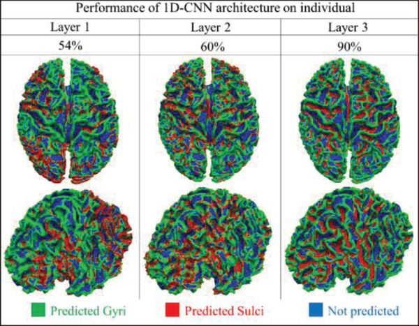
To present the classification performance, we pick up the same individual from each task and list the testing accuracy in Table 2. As we can observe from Table 2, quite high classification performances (nearly 90%) are achieved under different tasks. In addition, the average dice scores for gyri and sulci from task EMOTION are recorded accordingly, and they are 0.83 and 0.80. The classification performance of the individual brain is shown in layer 3 of Fig.6. In addition, the performance of each layer is also explored and summarized in Fig.6 to better understand the 1D CNN architecture. Other six tasks results are shown in the supplemental materials (Supplemental Figure 14). From Fig.6, we can see that most of the vertices we used can be differentiated correctly. The misclassified areas are varying on the different tasks and subjects. Similar to the analysis at group level, at the individual level, the architecture analysis algorithms are also adopted and results are interpreted for better understanding of how the CNN model discriminates gyral and sulcal fMRI signals. The architecture analysis of task EMOTION is shown in the Fig.7, and other six tasks achieved similar results, which are presented in supplemental materials (Supplemental Figure 15–20). In addition, to demonstrate the effectiveness and robustness of our model on the individual level, we applied our method to all the available individual subjects (60 subjects available in this work) for the HCP EMOTION task, and every subject shows consistently good classification performance. The average testing classification accuracy is about 0.913, and the standard deviation is 0.0071. This is another strong support that the functional differences of gyri/sulci truly exist, not only in the groupwise level, but also shown in the individual level.

Table.2.

Classification accuracy of each task at individual level.

Task	Classification accuracy	Task	Classification accuracy
EMOTION	92.1%	GAMBLING	89.2%
LANGUAGE	90.0%	MOTOR	89.0%
RELATIONAL	91.7%	SOCIAL	90.9%
WM	88.2%

Fig 6.

The classification performance of 3 convolutional layers in task EMOTION at individual level (one subject from task EMOTION). Each vertex is given a predicted label. Spatial maps of 2 different view angles are used to show the classification performance of each layer. Green vertices are predicted as gyri, red vertices are predicted as sulci, and blues ones are vertices that are not used.

Fig 7.

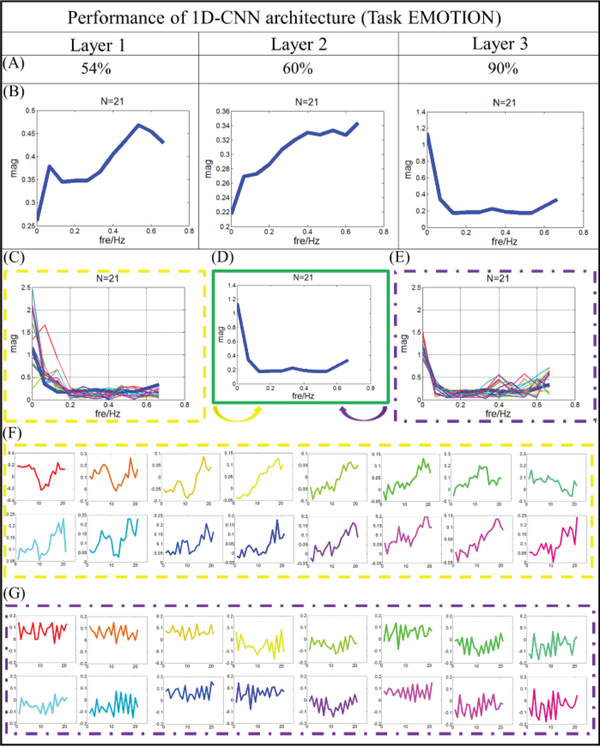
Filter feature analysis for task EMOTION. (A) Classification performance from layer 1 to 3. (B) The distribution of frequency for filter features in average level from layer 1 to 3. (C) The distribution of frequency for features from gyral filters. The distribution of frequency for the last layer is provided using bold blue line. (D) Distribution of frequency for the last layer. (E) The distribution of frequency for features from sulcal filters. The distribution of frequency for the last layer is provided using bold blue line. (F) Original features which are corresponding to (C), correspondence is presented by color. (G) Original features which are corresponding to (E), correspondence is presented by color.

Similar to the analysis at the group level, to elucidate the relationship between the distribution of frequency and classification accuracy, we went through all of the filters and features in each layer and present typical patterns for the last layer, as shown in Fig.7C-G. Two typical frequency patterns of the filter features are observed in the last layer: one has low frequency as shown in Fig. 7C, and another is relatively high with the pattern shown in Fig.7E. Their original features are extracted and presented in Fig.7F and Fig.7G, respectively. In contrast with the last layer, the pattern with low frequency is not discovered in the first two layers, hence, both patterns are indispensable to our classification, suggesting that they both contribute to the good classification performance in this experiment. Comparing with the results in Fig.5, quite consistent results are observed. Features with low frequency are observed in the gyral filters, but many higher frequency features are identified in the sulcal filters. In addition, the correlation coefficient of features in gyral filter is 0.67, however, the correlation coefficient is about 0.29 in the sulci filters. That means, at the individual level, the features in the gyral filter are much simpler and more consistent than the features in sulcal ones. This finding is quite consistent with conclusions we made from the group level.

C. Gyral and sulcal fMRI signals are largely different in resting state

We are interested in not only the task fMRI data but also the resting state fMRI (rsfMRI) data. To our knowledge, compared with task fMRI signals, the resting brain exhibits large scale functional oscillations among connected regions. Thus, we would like to explore whether gyral and sulcal fMRI signals are different in rsfMRI signals as well. We group 10 subjects’ rsfMRI data as the testbed to train the model and test the classification performance. In total, 10 subjects’ rsfMRI data (containing 600,000 rsfMRI time series with 1200 time points) are composited into a big data matrix to evaluate our CNN models (80% rsfMRI time series belong to the training samples and the rest are the testing ones, no overlap between training and testing samples). Following the structures, we mentioned in the method part, due to the huge dataset we are dealing with, the 1D CNN model in this section has 5 convolutional layers. The number of the filters in each layer is 64, 64, 64, 32 and 32, respectively. The main reason to use 5 layers is still about receptive field. The length of the inputs for the resting state fMRI is 1200 time points, which is 3–4 times longer than the task fMRI. In order to observe the differences among gyral/sulcal fMRI signals, more global receptive field for the filters may be needed. Usually, receptive field will become wider when the layers go deeper. Thus, one more layer is added in this section. Results demonstrated that a model with 5 layers works better. The parameters we used here are the same as those in the previous experiments.

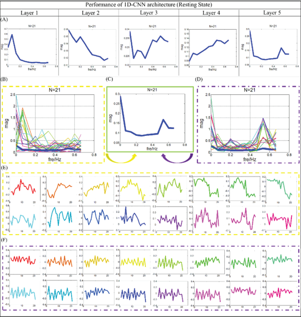
In the rsfMRI dataset, about 80.9% classification accuracy is observed at the group level. In addition, the average dice scores for gyri and sulci are recorded accordingly, which are 0.71 and 0.68. We map the predicted labels back onto each vertex, and then the classification performance of each individual is shown in Fig.8. Similar to the previous experiments, to unveil the characteristics of filter features in each layer, we went through all of the filters and features in each layer and presented typical patterns for the last layer. The results are presented in the Fig.9. As we can see from Fig.9, two typical patterns can be identified from Fig.9B and Fig.9D, and their original features are extracted and presented in Fig.9E and Fig.9F. Compared with the tfMRI dataset, quite similar patterns of filter feature in the last layer are observed. Notably, the correlation coefficient of features in gyral filter is 0.32, however, the correlation coefficient is about 0.22 in the sulci filters. That means, even in the rsfMRI dataset, the features in the gyral filter are much simpler and more consistent than the features in sulcal ones.

Fig 8.

The classification performances of 10 subjects in resting state. Each vertex on the surface is given a predicted label. Green vertices are predicted as gyri, red vertices are predicted as sulci, and blues ones are vertices that are not used. Zoom-in figures are used to show the performance of one case in 3 different directions.

Fig 9.

Filter feature analysis for resting state. (A) The distribution of frequency for filter features in average level from layer 1 to 5. (B) The distribution of frequency for features from gyral filters. The distribution of frequency for the last layer is provided using bold blue line. (C) Distribution of frequency for the last layer. (D) The distribution of frequency for features from sulcal filters. The distribution of frequency for the last layer is provided using bold blue line. (E) Original features which are corresponding to (B), and the correspondence is presented by color. (F) Original features which are corresponding to (D), and the correspondence is presented by color.

On the other hand, to demonstrate the effectiveness and robustness of our model at the individual level, we applied our method to all the available individual subjects (60 subjects available in this work) for the resting state fMRI, and every subject shows consistently good classification performance. The average classification performance is about 0.864, and the standard deviation is 0.0157, which consistently supports our conclusions. That is to say, no matter using tfMRI or rsfMRI, fMRI signals of gyri and sulci can be differentiated successfully. From what has been discussed above, we can draw a conclusion that gyri/sulci functional roles are fundamentally different in human brains, regardless of the brain conditions (e.g., task-based or task-free states). It is worth noting that the frequency differences between gyri and sulci are global across the whole cortical surface and our findings imply a systematic difference between gyrus and sulcus. Thus, even though the resting state fMRI signals from different individuals are considered as unique ones, features with frequency differences are robustly observed, and the powerful deep learning algorithms will learn the frequency differences and then summarize the meaningful features to differentiate the fMRI signals.

D. Gyral and sulcal fMRI signals are largely different in macaque brains

After analyzing the fMRI data of human brains, we also examined whether fMRI signals from their gyri and sulci are largely different in macaque monkey brains. In order to have larger dataset, in this experiment, we aggregated 6 macaques’ whole-brain fMRI signals together and there are about 80,000 rsfMRI temporal signals with hundreds of time points in total. We divided this big data matrix into training and testing samples (80% temporal signals are training samples and the left belongs to the testing samples, no overlap between training and testing samples). Here, the 1D CNN model in this section has 3 layers, and the number of the filters in each layer is 64, 32 and 32, respectively. Other parameters are the same as those used in the previous experiments.

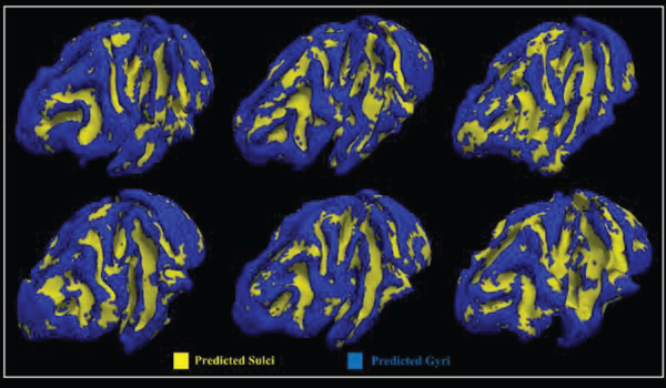
The testing accuracy of fMRI signals from gyri and sulci in macaque brains at group level is about 78.4%, which is reasonably good and consistent when compared with human brains. Furthermore, the average dice scores for gyri and sulci are recorded accordingly, which are about 0.64 and 0.58. As we can see the results from Fig.10, the classification performances are mapped back onto cortical surfaces of macaque brains, respectively. It is worth noting that here we predicted the whole brain cortical vertices with our trained CNN model for macaque brains since they have less complex folding patterns. The good classification performance strongly supports that there are fundamental functional differences between gyral signals and sulcal signals.

Fig 10.

The classification performances of 6 macaque brains. Each vertex on the surface is given a predicted label.

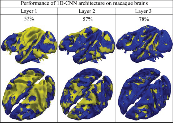
Like what we did in the previous sections, to explore the classification performance layer by layer, the performance of each layer is also explored and summarized in Fig.11 for better understanding of the 1D CNN architecture. From the Fig.11, we can see that the classification accuracy from layer 1 to 3 is 52%, 57% and 78%, respectively. The spatial maps of classification performance are also provided as the neuroanatomic reference. Similar as previous sections, the architecture analysis is adopted and the results are shown in Fig.12.

Fig 11.

The classification performances of 3 convolutional layers. (One subject from macaque brains). Each vertex will be given a predicted label, and gyral label is blue and sulcal label is yellow.

Fig 12.

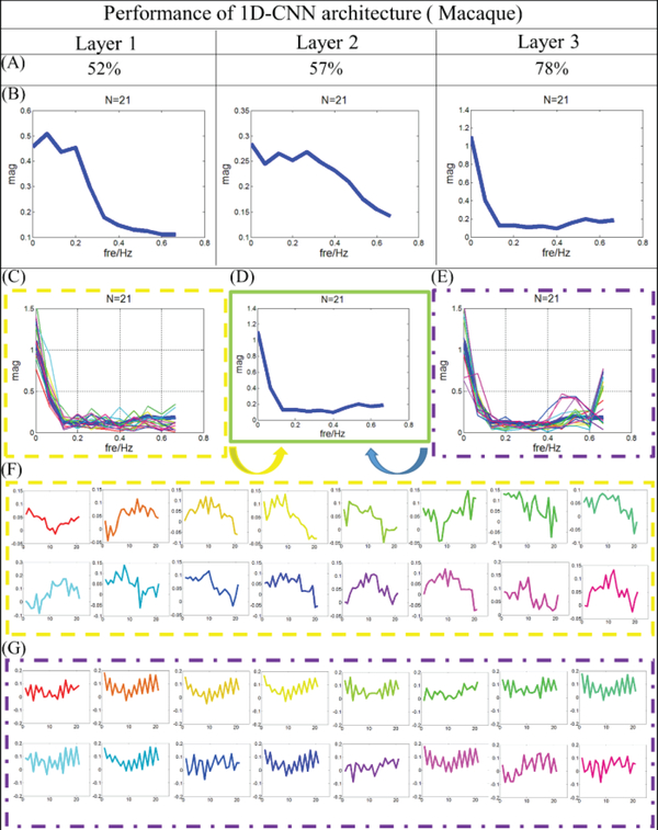
Filter feature analysis for macaque monkey brain. (A) Classification performance from layer 1 to 3. (B) The distribution of frequency for filter features in average level from layer 1 to 3. (C) The distribution of frequency for features from gyral filters. The distribution of frequency for the last layer is provided using bold blue line. (D) Distribution of frequency for the last layer. (E) The distribution of frequency for features from sulcal filters. The distribution of frequency for the last layer is provided using bold blue line. (F) Original features which are corresponding to (C), and the correspondence is presented by color. (G) Original features which are corresponding to (E), and the correspondence is presented by color.

Two typical frequency patterns of the filter features are still observed in the last layer: one has low frequency as shown in Fig. 12C, and another is relatively high with the pattern demonstrated in Fig.12E. Their original features are extracted and presented in Fig.12F and Fig.12G, respectively. Compared with the results in Figs.5, 7 and 9, consistent results are observed. Features with low frequency are observed in the gyral filters, but high frequency features are identified in the sulcal filters. However, different from the results of human brains, the correlation coefficient of features in gyral filter is about 0.3, which is a 5% smaller than the correlation coefficient of features in sulcal filter. This is reasonable as in the resting state fMRI scans, brains are not under specific tasks, and thus their gyral signals may not quite follow certain global functions and then their gyral signals may not be that globally consistent. Another possible reason might be that these macaque brains are still growing, and the gyral filters may become more globally consistent after the macaques are grown up. Generally speaking, gyral signals and sulcal signals still can be distinguished very well even in the six-month macaque brains. It reveals again that gyri and sulci have fundamentally different functional roles and they are differentiable by CNN deep learning models.

IV. Conclusion

In this paper, we proposed a data-driven computational framework of 1D CNN to classify and interpret the gyral and sulcal fMRI signals in multiple different experiments. An average of 83% and 90% classification accuracy has been achieved to separate gyral/sulcal HCP task fMRI signals at the population and individual subject level; 81% and 86% classification accuracy for resting state fMRI signals at the group and individual subject level. 78% classification accuracy has been achieved to separate gyral/sulcal resting state fMRI signals in macaque brains. In addition, we explored the trained CNN models layer by layer and interpreted the features learned by CNN. Our results demonstrated that the CNN models have the ability to differentiate gyral and sulcal fMRI signals, and gyral features are simpler and more related to the lower frequency features when compared with the fMRI signals on sulci. That is, frequency of fMRI signals in gyri is lower. The possible reason is that gyri exchange information among remote structurally connected gyri. On the contrary, sulci have higher frequency since sulci communicate directly with their neighboring gyri and indirectly with other cortical regions through gyri. Thus, to communicate with others, gyri usually have a lower frequency but sulci have higher ones.

By using the 1D CNN algorithm to differentiate the gyral/sulcal fMRI signals, we don’t need to manually design any feature, deep learning will automatically perform the high-level feature abstractions, which includes much more meaningful and less noisy features. And those features from different layers can represent the typical pattern of the inputs somehow (even features are hard to discover directly). Hence, using the feature from the deeper layers to classify the inputs into categories are the key step to pursuit the desirable classification performance. Our future works will focus on the exploration of the possible mechanisms that underlie the different functional roles of gyri and sulci on more specific regions. Another possible future work will be the investigation of how such difference is altered in brain disorders such as Autism and Schizophrenia.

References

- [1].Cachia A, Mangin JF, Rivière D, et al. (2003). A generic framework for the parcellation of the cortical surface into gyri using geodesic Voronoi diagrams. Medical Image Analysis, 7(4): 403–416. [DOI] [PubMed] [Google Scholar]
- [2].Chi JG, Dooling EC, Gilles FH. (1977). Gyral development of the human brain. Annals of neurology, 1(1): 86–93. [DOI] [PubMed] [Google Scholar]
- [3].Desikan RS, Ségonne F, Fischl B, et al. (2006). An automated labeling system for subdividing the human cerebral cortex on MRI scans into gyral based regions of interest. Neuroimage, 31(3): 968–980. [DOI] [PubMed] [Google Scholar]
- [4].Destrieux C, Fischl B, Dale A, et al. (2010). Automatic parcellation of human cortical gyri and sulci using standard anatomical nomenclature. Neuroimage, 53(1): 1–15. [DOI] [PMC free article] [PubMed] [Google Scholar]
- [5].Fischl B, Sereno M, Dale AM. (1999). Cortical surface-based analysis II: inflation, flattening, and a surface-based coordinate system. NeuroImage, 9(2):195–207. [DOI] [PubMed] [Google Scholar]
- [6].Fischl B, Van Der Kouwe A, Destrieux C, et al. (2004). Automatically parcellating the human cerebral cortex. Cerebral cortex, 14(1): 11–22. [DOI] [PubMed] [Google Scholar]
- [7].Liu T (2011). A few thoughts on brain ROIs. Brain Imaging and Behav, 5(3):189–202. [DOI] [PMC free article] [PubMed] [Google Scholar]
- [8].Thirion JP (1996). The extremal mesh and understanding of 3D surfaces. Int J Comput Vis, 19(2):115–128. [Google Scholar]
- [9].Van Essen DC, (1997). A tension-based theory of morphogenesis and compact wiring in the central nervous system. Nature, 385, 313–318. [DOI] [PubMed] [Google Scholar]
- [10].Jalil Razavi M, Zhang T, Liu T et al. 2015. Cortical Folding Pattern and its Consistency Induced by Biological Growth. Scientific reports. 5:14477. [DOI] [PMC free article] [PubMed] [Google Scholar]
- [11].Tallinen T, Chung JY, Rousseau F et al. 2016. On the growth and form of cortical convolutions. Nature Physics. 12:588. [Google Scholar]
- [12].Barkovich AJ, Guerrini R, Kuzniecky RI et al. 2012. A developmental and genetic classification for malformations of cortical development: update 2012. Brain : a journal of neurology. 135:1348–1369. [DOI] [PMC free article] [PubMed] [Google Scholar]
- [13].Stahl R, Walcher T, De Juan Romero C et al. 2013. Trnp1 regulates expansion and folding of the mammalian cerebral cortex by control of radial glial fate. Cell. 153:535–549. [DOI] [PubMed] [Google Scholar]
- [14].Zhang T, Razavi MJ, Chen H et al. 2017. Mechanisms of circumferential gyral convolution in primate brains. Journal of Computational Neuroscience. 42:217–229. [DOI] [PubMed] [Google Scholar]
- [15].Öngür D, Price JL. (2000). The organization of networks within the orbital and medial prefrontal cortex of rats, monkeys and humans. Cerebral cortex, 10(3): 206–219. [DOI] [PubMed] [Google Scholar]
- [16].Schleicher A, Morosan P, Amunts K, et al. (2009). Quantitative architectural analysis: a new approach to cortical mapping. Journal of autism and developmental disorders, 39(11): 1568–1581. [DOI] [PubMed] [Google Scholar]
- [17].Van Essen DC, (2013). Cartography and connectomes. Neuron, 80(3), 775–790. [DOI] [PMC free article] [PubMed] [Google Scholar]
- [18].Deng F, Jiang X, Zhu D, et al. (2014). A functional model of cortical gyri and sulci. Brain structure & function, 219, 1473–1491. [DOI] [PMC free article] [PubMed] [Google Scholar]
- [19].Ge F, Li X, Razavi MJ, et al. (2017). Denser Growing Fiber Connections Induce 3-hinge Gyral Folding. Cerebral Cortex: 1–12. [DOI] [PMC free article] [PubMed] [Google Scholar]
- [20].Liu H, Jiang X, Zhang T, et al. (2017). Elucidating Functional Differences between Cortical Gyri and Sulci via Sparse Representation HCP Grayordinate fMRI Data. Brain Research. [DOI] [PMC free article] [PubMed] [Google Scholar]
- [21].Nie J, Guo L, Li K, et al. (2012). Axonal fiber terminations concentrate on gyri. Cerebral Cortex, 22(12):2831–9. [DOI] [PMC free article] [PubMed] [Google Scholar]
- [22].Chen H, Zhang T, Guo L, et al. (2012). Coevolution of gyral folding and structural connection patterns in primate brains. Cerebral Cortex, 23(5): 1208–1217. [DOI] [PMC free article] [PubMed] [Google Scholar]
- [23].Jiang X, Li X, Lv J, et al. (2015). Sparse representation of HCP grayordinate data reveals novel functional architecture of cerebral cortex. Human brain mapping, 36(12): 5301–5319. [DOI] [PMC free article] [PubMed] [Google Scholar]
- [24].Jiang X, Li X, Lv J, et al. (2016). Temporal dynamics assessment of spatial overlap pattern of functional brain networks reveals novel functional architecture of cerebral cortex. IEEE Transactions on Biomedical Engineering. [DOI] [PMC free article] [PubMed] [Google Scholar]
- [25].Stephan T, Deutschländer A, Nolte A, et al. (2005). Functional MRI of galvanic vestibular stimulation with alternating currents at different frequencies. Neuroimage, 26(3): 721–732. [DOI] [PubMed] [Google Scholar]
- [26].Goldberg JM, Smith CE, Fernandez C (1984). Relation between discharge regularity and responses to externally applied galvanic currentsin vestibular nerve afferents of squirrel monkey. J. Neurophysiol. 51,1236–1256. [DOI] [PubMed] [Google Scholar]
- [27].Kleine JF, Guldin OW, Clarke AH, (1999). Variable otolith contribution to the galvanically induced vestibulo-ocular reflex. NeuroReport 10, 1143–1148. [DOI] [PubMed] [Google Scholar]
- [28].Kandel ER, Schwartz JH, Jessell TM. (2000). Principles of Neural Science, the fourth edition.
- [29].Passingham RE, Stephan KE, Kötter R. (2002). The anatomical basis of functional localization in the cortex. Nat Rev Neurosci, 3(8):606–616. [DOI] [PubMed] [Google Scholar]
- [30].Zilles K, Amunts K. (2009). Centenary of Brodmann’s map--conception and fate. Nat Rev Neurosci, 11(2):139–145. [DOI] [PubMed] [Google Scholar]
- [31].Bengio Y, Courville A. (2012). Vincent P: Representation Learning: A Review and New Perspectives. IEEE Trans. Pattern Anal. Mach. Intell, 35, 1798–1828. [DOI] [PubMed] [Google Scholar]
- [32].Deng L, Li J, Huang JT, et al. (2013). Recent advances in deep learning for speech research at Microsoft. Acoustics, Speech and Signal Processing (ICASSP), 2013 IEEE International Conference on IEEE: 8604–8608. [Google Scholar]
- [33].LeCun Y, Bengio Y, Hinton G. (2015). Deep learning. Nature, 521(7553): 436–444. [DOI] [PubMed] [Google Scholar]
- [34].Schmidhuber J (2015). Deep learning in neural networks: An overview. Neural networks, 61: 85–117. [DOI] [PubMed] [Google Scholar]
- [35].Socher R, Huval B, Bath B, et al. (2012). Convolutional-recursive deep learning for 3d object classification. Advances in Neural Information Processing Systems: 656–664. [Google Scholar]
- [36].Sun Y, Wang X, Tang X. (2014). Deep learning face representation from predicting 10,000 classes. Proceedings of the IEEE Conference on Computer Vision and Pattern Recognition: 1891–1898. [Google Scholar]
- [37].Wan J, Wang D, Hoi SCH, et al. (2014). Deep learning for content-based image retrieval: A comprehensive study. Proceedings of the 22nd ACM international conference on Multimedia ACM: 157–166. [Google Scholar]
- [38].Ciregan D, Meier U, Schmidhuber J. (2012). Multi-column deep neural networks for image classification. Computer Vision and Pattern Recognition (CVPR), 2012 IEEE Conference on IEEE: 3642–3649. [Google Scholar]
- [39].Ciresan DC, Meier U, Masci J, et al. (2011). Flexible, high performance convolutional neural networks for image classification. Twenty-Second International Joint Conference on Artificial Intelligence. [Google Scholar]
- [40].Jaderberg M, Vedaldi A, Zisserman A. (2014). Deep features for text spotting. European conference on computer vision. Springer International Publishing: 512–528. [Google Scholar]
- [41].Karpathy A, Toderici G, et al. (2014). Large-scale video classification with convolutional neural networks. Proceedings of the IEEE conference on Computer Vision and Pattern Recognition: 1725–1732. [Google Scholar]
- [42].Krizhevsky A, Sutskever I, Hinton GE. (2012). Imagenet classification with deep convolutional neural networks. Advances in neural information processing systems. 1097–1105. [Google Scholar]
- [43].Hoo-Chang S, Roth HR, et al. (2016). Deep convolutional neural networks for computer-aided detection: CNN architectures, dataset characteristics and transfer learning. TMI. 1285. [DOI] [PMC free article] [PubMed] [Google Scholar]
- [44].Lai S, Xu L, Liu K, et al. (2015). Recurrent Convolutional Neural Networks for Text Classification. AAAI, 333: 2267–2273. [Google Scholar]
- [45].Wang T, Wu DJ, Coates A, et al. (2012). End-to-end text recognition with convolutional neural networks. Pattern Recognition (ICPR), 2012 21st International Conference on IEEE: 3304–3308. [Google Scholar]
- [46].Huang H, Hu X, Makkie M, et al. (2017). Modeling Task fMRI Data via Deep Convolutional Autoencoder. IEEE Trans Med Imaging: 411–424 [DOI] [PubMed] [Google Scholar]
- [47].Sarraf S, Tofighi G. (2016). Classification of alzheimer’s disease using fmri data and deep learning convolutional neural networks. arXiv preprint arXiv:1603.08631. [Google Scholar]
- [48].Suk HI, Shen D. (2013). Deep learning-based feature representation for AD/MCI classification. International Conference on Medical Image Computing and Computer-Assisted Intervention Springer Berlin Heidelberg: 583–590. [DOI] [PMC free article] [PubMed] [Google Scholar]
- [49].Suk HI, Lee SW, Shen D, et al. (2014). Hierarchical feature representation and multimodal fusion with deep learning for AD/MCI diagnosis. NeuroImage, 101: 569–582. [DOI] [PMC free article] [PubMed] [Google Scholar]
- [50].Zhao Y, Dong Q, Zhang S, et al. (2017). Automatic Recognition of fMRI-derived Functional Networks using 3D Convolutional Neural Networks. IEEE Transactions on Biomedical Engineering. [DOI] [PMC free article] [PubMed] [Google Scholar]
- [51].Li K, Guo L, Li G, et al. (2009) Gyral folding pattern analysis via surface profiling. International Conference on Medical Image Computing and Computer-Assisted Intervention Springer, Berlin, Heidelberg: 313–320. [DOI] [PMC free article] [PubMed] [Google Scholar]
- [52].Glasser Matthew F., Sotiropoulos Stamatios N., Wilson J. Anthony, et al. (2013). The minimal preprocessing pipelines for the Human Connectome Project. Neuroimage 80: 105–124. [DOI] [PMC free article] [PubMed] [Google Scholar]
- [53].Woolrich MW, Ripley BD, et al. (2001). Temporal autocorrelation in univariate linear modelling of FMRI data. NeuroImage, 14(6):1370–1386. [DOI] [PubMed] [Google Scholar]
- [54].Lv J, et al. (2015). Holistic atlases of functional networks and interactions reveal reciprocal organizational architecture of cortical function. IEEE Transactions on Biomedical Engineering, 62(4): 1120–1131. [DOI] [PubMed] [Google Scholar]
- [55].Liu T, et al. (2007). “Brain tissue segmentation based on DTI data.” NeuroImage 381: 114–123. [DOI] [PMC free article] [PubMed] [Google Scholar]
- [56].Liu T, Nie J, Tarokh A, Guo L, Wong ST. (2008). Reconstruction of central cortical surface from brain MRI images: method and application. NeuroImage. Apr 15;40(3):991–1002. [DOI] [PMC free article] [PubMed] [Google Scholar]
- [57].Li K, Guo L, Li G, et al. (2010). Cortical surface based identification of brain networks using high spatial resolution resting state fMRI data. InBiomedical Imaging: From Nano to Macro, 2010 IEEE International Symposium (pp. 656–659). IEEE. [Google Scholar]
Associated Data
This section collects any data citations, data availability statements, or supplementary materials included in this article.