Abstract
Background
Sample size calculations are critical to the planning of a clinical trial. For single-arm trials with time-to-event endpoint, standard software provides only limited options. The most popular option is the log-rank test. A second option assuming exponential distribution is available on some online websites. Both these approaches rely on asymptotic normality for the test statistic and perform well for moderate-to-large sample sizes.
Methods
As many new treatments in the field of oncology are cost-prohibitive and have slow accrual rates, researchers are often faced with the restriction of conducting single arm trials with potentially small-to-moderate sample sizes. As a practical solution, therefore, we consider the option of performing the sample size calculations using an exact parametric test with the test statistic following a chi-square distribution. Analytic results of sample size calculations from the two methods with Weibull distributed survival times are briefly compared using an example of a clinical trial on cholangiocarcinoma and are verified through simulations.
Results
Our simulations suggest that in the case of small sample phase II studies, there can be some practical benefits in using the exact test that could affect the feasibility, timeliness, financial support, and ‘clinical novelty’ factor in conducting a study. The exact test is a good option for designing small-to-moderate sample trials when accrual and follow-up time are adequate.
Conclusions
Based on our simulations for small sample studies, we conclude that a statistician should assess sensitivity of his calculations obtained through different methods before recommending a sample size to their collaborators.
Keywords: Clinical trial, Exact test, Single-arm, Survival, Weibull
1. Introduction
Two-arm randomized clinical trials are the gold standard in biomedical research as they allow performance assessment of a new experimental treatment relative to a standard control. However, there are situations where conducting a two-arm trial is not possible and a single-arm trial may be the preferred choice. For single-arm trials with a time-to-event endpoint, surprisingly few options for sample size calculation are available in literature or in standard software. The most popular option is the log-rank test [1] and its weighted versions. It has been used for sample size calculations by Finkelstein et al. [2], Kwak and Jung [3], Jung [4], Sun et al. [5] and more recently by Wu [6]. Likewise, sample size calculations for exponentially distributed survival times have been proposed by Lawless [7] (available as online calculators; see SWOG [8]). Both approaches rely on asymptotic normality of the test statistic and perform well for moderate-to-large sample sizes. As many new treatments in the field of oncology are cost-prohibitive and have slow accrual rates, researchers are often restricted to conducting single-arm trials with small-to-moderate sample sizes.
The sample size formula proposed by Wu [6] is based on the exact variance of the test statistic and hence is an improvement on the earlier versions of the logrank test. Wu [6] has mentioned in his concluding remarks that his one-sample logrank test is conservative when dealing with small samples and that the correctness of its use depends on the correct specification of the underlying distribution of the standard population. In this context, we bring to the reader's attention that a parametric method of calculating sample size for exponentially distributed times was first published by Epstein and Sobel [9]. This method uses a test statistic that follows a chi-square distribution. Later, Narula and Li [10] have shown how to extend the calculations to the case of gamma, Weibull, and Laplace distributions in the uncensored case. One important point to note is that an iterative search algorithm may be needed to calculate the sample size given the value the other fixed parameters using their approach and to avoid this Narula and Li [10] also mention five different closed-form solutions based on a normal approximation. Surprisingly, popular statistics software does not have options for such calculations though PASS [11] has incorporated the logrank calculations of Wu [6].
2. Methods
The Weibull distribution is a two-parameter distribution with its pdf given by:
| (1) |
here is a scale parameter and is a shape parameter that determines the shape of the hazard function ( gives hazard that is increasing over time, and, gives hazard that is decreasing over time with representing the special case of exponential distribution with constant hazard).
With modern computational tools, we can write an efficient SAS program for an iterative approach using the formula given in Narula and Li [10] accounting for administrative censoring. That is, following Narula and Li [10], the problem of calculating sample size n (without censoring) in the Weibull case to test the hypothesis against the alternative at level of significance and probability of type II error reduces to solving for using
| (2) |
with and . Our program then adjusts their method for administrative censoring accounting for study-specific accrual and follow-up times in the following way:
Assuming a uniform accrual, the censoring distribution function is given by
| (3) |
where and are the accrual and follow-up time respectively. Then the probability that a subject experiences a failure during the study is given by
| (4) |
where is with . Dividing the number of events by gives the sample size adjusted for administrative censoring. Alternatively, can be calculated using Simpson's rule by
| (5) |
where is the survival function of the Weibull with
For the Weibull, this allows comparison with Wu [6] and for the special case of the exponential, this allows comparison with Lawless [7]. To do so, we consider a real-life example about designing a phase II clinical trial for treating patients suffering from chemotherapy refractory advanced metastatic biliary cholangiocarcinoma, a “rare” but aggressive neoplasm. Such patients have metastatic disease and undergo an initial treatment followed by a second-line treatment which has a progression-free survival (PFS) rate of 5–10% by 1 year. Oncologists are therefore working towards improving the PFS by using new combination therapies. Historically, published literature mentions a median PFS of 2.5 months with an IQR of around 2–5 months. Due to dismal survival rates, they consider an improvement in 25th, 50th and 75th percentile of PFS by a factor of 1.5 as clinically meaningful and holding promise for future large sample studies. The rarity of disease poses recruitment problems with typical accrual rates being approximately 12–15 patients/year. Based on financial and administrative limitations, researchers envision a study with an accrual time of 2 years and follow-up time of 3 years. Loss to follow-up is anticipated to be 15–20%. It should be noted that as the researchers hypothesize a consistent improvement in PFS for all quantiles of the survival curve - of the historical controls by a factor of 1.5, the Weibull distribution is a good choice for performing the sample size calculations as is evident from the definition of in (1). Following Wu [6], the shape parameter for the Weibull is estimated from the historical controls as 1.25 (increasing hazard).
3. Results
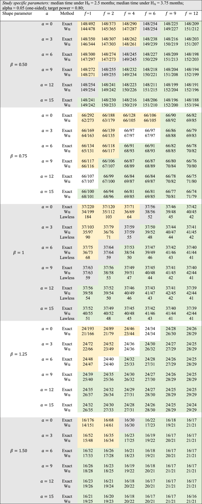
For the study-specific design features in this example, Table 1 shows the comparisons between the two methods for various values of the shape parameter ranging from 0.5 to 1.5. The conservative nature of the logrank test can be studied by observing how in Table 1 the sample sizes vary as a function of accrual and follow-up time (keeping other design parameters fixed) for the different values of the shape parameter. When = 0.5, we see that Wu's logrank test gives smaller sample sizes compared to the exact method only when both and are small in magnitude. On the other hand, as either or increases, the exact test yields smaller sample sizes. This general pattern is even more accentuated as increases from 0.5 to 1.5. In fact, for = 1.5, only and allow the logrank test to have smaller sample sizes than the exact method. As in the cholangiocarcinoma example under consideration, researchers hypothesize improvement in median PFS by a factor of 1.5, small values of and are impractical as based on the accrual rate, very few patients can participate in this study.
Table 1.
Number of events/sample size for exact vs Wu's method (administrative censoring adjustment by equation [4]) for different values of Weibull shape parameter , accrual time , and follow-up time .
For this example, where = 1.25 is chosen, the exact method gives a sample size of 24 when and whereas the logrank test finds a lower bound at 29 no matter how big and are chosen. That is, even with the flexibility to follow patients for a hypothetically large amount of time and thereby observe all events, Wu's method does not go below a threshold value of 29 events. Through simulations (we used 10,000 simulations) using the Weibull distribution, it can be shown that with large follow-up times, 80% power is achieved only with 24 subjects and the exact method is analytically able to yield a sample size of 24. By adopting the popular ad-hoc method of inflating the sample size to accommodate drop-outs (conservatively assuming they provide no extra information), the adjusted sample size can be calculated as 24/0.8 = 30. That is, if the researcher's ‘optimistic’ estimate of accruing 15 patients/year is true, it appears likely that this study can be completed within the stipulated timeframe. A similar ad-hoc adjustment for Wu's method would require 37 patients to be enrolled, which is outside the practical timeframe of the study. However, by assuming that drop-outs occur randomly over the study period (assuming a uniform distribution), for an anticipated drop-out rate of 20%, our simulations gave a sample size of n = 28 with 80.6% power. Thus, a combination of analytical calculations using the exact method aided by further simulations can enable a statistician to design a small sample trial with adequate power. If additional information from similar such studies is available, a statistician can also incorporate other drop-out mechanisms (such as exponentially distributed drop-out times with a specific mean).
Similar comparisons can be performed for other values of such as = 0.75 (decreasing hazard) and = 1 (constant hazard – exponential distribution). In the case of = 1, it can be seen that the normal approximation proposed by Lawless [7] gives smaller n than the exact method for small-to-moderate values of follow-up time. However, with large values of follow-up time, this is no longer the case and the normal approximation cannot yield sample sizes below n = 41. Through simulations (we used 10,000 simulations) using the exponential distribution, it can be shown that with large follow-up times, 80% power is achieved only with 37 subjects and the exact method is analytically able to yield a sample size of 37 whereas the normal approximation method and the logrank test yield sample sizes of 40 and 43 respectively.
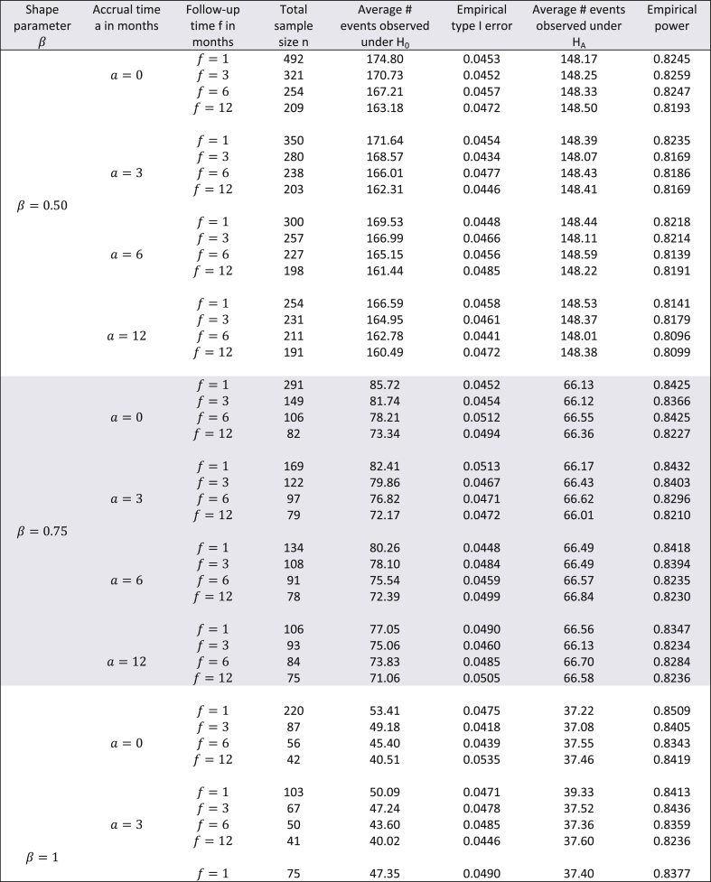
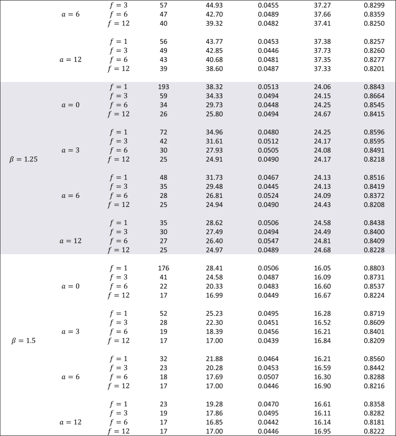
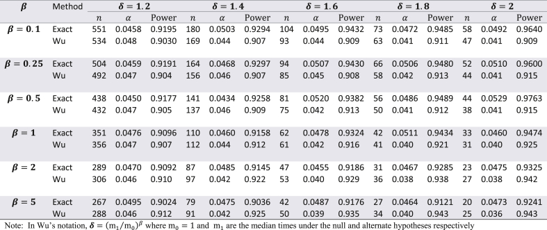
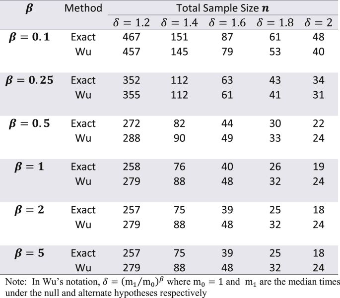
Though the exact method yields smaller sample sizes for many situations, it is necessary to assess whether or not the empirical type I error rate and empirical power are close to their nominal values. To do this, a simulation study (with 10,000 simulations) was conducted with the study-specific design parameters of the cholangiocarcinoma study. For varying values of and for ranging from 0.5 to 1.5, time-to-event data was simulated with the sample sizes calculated by the exact method and the results are displayed in Table 2. From this table it can be see that for almost all scenarios the empirical type I error rates were close to the nominal 5% alpha level. Likewise, empirical power always slightly exceeded the target 80% power. Except for seemingly impractical values such as (all subjects are available for recruitment at the start) and (a very short follow-up time for the study under consideration), there was not much difference in the magnitude by which empirical power exceeded the target power. As the results displayed in Table 2 are in the context of a specific example with a fixed effect size, a similar evaluation of empirical type I error and power was conducted for the hypothetical example discussed in Wu [6] where in and was kept fixed, but the effect size was varied from small to large, for = 0.1, 0.25, 0.5, 1, 2, and 5. The results of these simulations are shown in Table 3 with target power at 90% and median time under the null hypothesis fixed at 1. Here too, for all scenarios, empirical type I error was close to the nominal level, and likewise, empirical power always slightly exceeded the 90% target level. For , the exact method yielded somewhat higher empirical power compared to Wu's method, while the converse was true for . Though at first glance Table 3 suggests that the exact method yields smaller sample sizes than the logrank test (with both methods having comparable empirical type I error and power) only for , it should be noted that the combination of and represent values that are quite small compared to the magnitude of the hypothesized improvement in median lifetime under the alternate hypothesis. For example, the combination of and indicates that the median under the alternate hypothesis is 6.55 times the median under the null (which is fixed at 1). Likewise, the combination of and indicates that the median under the alternate hypothesis is 1024 times the median under the null (which is fixed at 1). Thus, in such scenarios, it would be impractical to choose small values of and . As the values of and increase, compared to the logrank test, the exact method gives smaller sample sizes for and same sample sizes for (see results in Table 4). Though the logrank test gives smaller sample sizes for , such a small value of the shape parameter would require a very strong justification in a real life clinical trial.
Table 2.
Evaluation of empirical type I error and empirical power using the exact method for the cholangiocarcinoma study with months and effect size equal to improvement in median time by a factor of 1.5 - using 10,000 simulations (nominal type I error 5%, target power 80%).
Table 3.
Comparing empirical type I error and empirical power with Wu's method for the example in Wu (2015 – accrual time = 3, follow-up time = 1, nominal type I error 5%, nominal power 90%)) using the exact adjustment for administrative censoring given by equation (4) – number of simulations = 10,000.
Table 4.
Sample size comparison of exact vs Wu's method for the example in Wu (2015) – with a = 18, f = 18 (all other parameters same as Table 3).
For all results discussed in this section we used equation (4) to adjust for administrative censoring. For all scenarios shown in Table 3, we got very similar sample sizes (mostly same, sometimes differing by 1, rarely differing by 2) whether we used equation (4) or Simpson's rule mentioned in equation (5) except in the case when . In this case, adjustment by Simpson's rule yielded sample sizes of 284, 84, 44, 27 and 20 for 1.2, 1.4, 1.6, 1.8 and 2 respectively. We thus recommend adjusting for administrative censoring using equation (4).
4. Conclusion
For large phase II or III trials, it would not make much difference if any of these three methods were used for sample size calculations. However, in the case of small sample phase II studies, there could be practical differences that would affect the feasibility, timeliness, financial support, and ‘clinical novelty’ factor (the challenge faced by clinicians to be the first to conduct a clinical trial using a novel idea) of the study. Additionally, both Wu's method and Lawless' method do not yield sample sizes below a certain threshold no matter how long the accrual and follow-up times are. On the other hand, the exact method does not suffer from this shortcoming. As for the concluding remark by Wu [6] about correctly specifying the underlying distribution, we fully agree with this assertion. In this context, we provide two insights. The first is the possibility to extend the framework presented in Narula and Li [10] to using a generalized gamma distribution (a family of distributions with exponential, Weibull, lognormal, gamma, inverse-Weibull, and inverse-gamma, as special cases) to model the historical controls in the case where definitive well-established large sample studies have been conducted on such historical controls and then use the estimates of these parameters to design the current single-arm study. Just like the gamma, Weibull and Laplace distributions, the sample size calculation could be done using the framework presented in Narula and Li [10] as it would allow calculation of (in place of n in equation (1)) where is the extra shape parameter estimated from historical controls. Then dividing by would yield the sample size required for current single-arm study. The second insight is to conduct simulations during the design phase of a study to assess how, in the case of Weibull, partial information available from historical data impacts the sample size calculation for the current study. Often, historical control information is available in published literature in the form of a Kaplan Meier curve, or as point estimates of median and/or interquartile range. It would therefore be interesting to assess the sensitivity of using this partial information from prior studies on the sample size calculations of the current study. Additionally, the role of random censoring due to drop-outs/loss to follow-up needs to be addressed in a comprehensive manner.
In some disease-specific areas, single-arm trials are inevitable. For example, conducting a randomized controlled trial (RCT) may prove impractical when recruiting a small target population (rare disease). Ethical or practical considerations may dictate that researchers conduct a single-arm trial with all enrolled patients receiving the experimental treatment. Another example of a single-arm trial is the “window-of-opportunity” trial in which patients diagnosed with a disease are awaiting subsequent surgery and can be enrolled only in this waiting period. The number of such patients may be small requiring a single-arm study. Likewise, there are situations where the standard drug has been so well studied and documented that researchers may consider published results about its performance as reliable historical data. In this case, they may prefer a single-arm trial. Further, in the case of some rare diseases, it may be ethical to treat only those subjects with a new experimental drug who have stabilized on the standard-of-care treatment, thereby warranting a single-arm study.
Overall, we feel that statisticians should be aware of the issues we have discussed in planning a single-arm trial for time-to-event data. Our calculations and simulation study suggests that the exact method is a good option for designing small-to-moderate sample trials when accrual and follow-up time is adequate. Thus, in cancer trials where accrual rates are low, it may be necessary to have longer accrual times and in such trials, the exact method may be preferred as it yields smaller sample sizes with sufficient power while maintaining the type I error rate. The statistician should strive to use the most appropriate method considering various practical considerations in consultation with the researchers. Especially, in the case of small sample studies, they should assess sensitivity of their calculations obtained through different methods.
Acknowledgement
None.
Footnotes
Supplementary data to this article can be found online at https://doi.org/10.1016/j.conctc.2019.100360.
Disclosure
The author has no relevant conflicts of interest to declare.
Appendix A. Supplementary data
The following is the Supplementary data to this article:
References
- 1.Breslow N.E. Analysis of survival data under the proportional hazards model. Int. Stat. Rev. 1975;43:44–58. [Google Scholar]
- 2.Finkelstein D.M., Muzikansky A., Schoenfeld D.A. Comparing survival of a sample to that of a standard population. J. Natl. Cancer Inst. 2003;95:1434–1439. doi: 10.1093/jnci/djg052. [DOI] [PubMed] [Google Scholar]
- 3.Kwak M., Jung S.H. Phase II clinical trials with time-to-event endpoints: optimal two-stage designs with one-sample log-rank test. Stat. Med. 2014;33:2004–2016. doi: 10.1002/sim.6073. [DOI] [PMC free article] [PubMed] [Google Scholar]
- 4.Jung S.H. CRC Press: Chapman and Hall; 2013. Randomized Phase II Cancer Clinical Trial. [Google Scholar]
- 5.Sun X., Peng P., Tu D. Phase II cancer clinical trials with a one-sample log-rabk test and its corrections based on the Edgeworth expansion. Contemp. Clin. Trials. 2011;32:108–113. doi: 10.1016/j.cct.2010.09.009. [DOI] [PubMed] [Google Scholar]
- 6.Wu J. Sample size calculation for the one-sample log-rank test. Pharmaceut. Stat. 2015;14:26–33. doi: 10.1002/pst.1654. [DOI] [PubMed] [Google Scholar]
- 7.Lawless J.F. second ed. John Wiley and Sons; New York: 2003. Statistical Models and Methods for Lifetime Data. [Google Scholar]
- 8.SWOG: Cancer Research Network – Cancer Research and Biostatistics. https://stattools.crab.org/Calculators/oneArmSurvivalColored.html Available at:
- 9.Epstein B., Sobel M. Life testing. J. Am. Stat. Assoc. 1953;48(263):486–582. [Google Scholar]
- 10.Narula S.C., Li F.S. Sample size calculations in exponential life testing. Technometrics. 1975;17(2):229–231. [Google Scholar]
- 11.PASS 14 Power Analysis and Sample Size Software. NCSS, LLC; Kaysville, Utah, USA: 2015. ncss.com/software/pass. [Google Scholar]
Associated Data
This section collects any data citations, data availability statements, or supplementary materials included in this article.


