Evolutionary Modeling in SLiM 3 for Beginners

Abstract

The SLiM forward genetic simulation framework has proved to be a powerful and flexible tool for population genetic modeling. However, as a complex piece of software with many features that allow simulating a diverse assortment of evolutionary models, its initial learning curve can be difficult. Here we provide a step-by-step demonstration of how to build a simple evolutionary model in SLiM 3, to help new users get started. We will begin with a panmictic neutral model, and build up to a model of the evolution of a polygenic quantitative trait under selection for an environmental phenotypic optimum.

Introduction

Forward genetic simulations play a central role in modern population genetics and evolutionary biology (Carvajal-Rodriguez 2010; Yuan et al. 2012; Bank et al. 2014; Hoban 2014; Thornton 2014; Haller and Messer 2017a, 2019; Haller et al. 2019). Such simulations can be used to investigate a remarkable variety of research questions, from predicting the evolutionary dynamics of real populations (Kosheleva and Desai 2018; Matz et al. 2018; Rougemont et al. 2018) to testing hypotheses about past evolutionary mechanisms (Nowak et al. 2014; Fijarczyk et al. 2018; Pouyet et al. 2018), validating statistical or empirical methods (Haller and Messer 2017b; Henden et al. 2018; Librado and Orlando 2018), and exploring the evolutionary consequences of theoretical ideas (Champer et al. 2018; Kim et al. 2018; Parada and Charlesworth 2018).

The SLiM forward genetic simulation framework has become a popular tool for constructing such models due to the power and flexibility provided by its scriptability in the Eidos language, as well as its incorporation of SLiMgui, an interactive graphical modeling environment (Messer 2013; Haller and Messer 2017a, 2019). However, with the SLiM manual (Haller and Messer 2016) and Eidos manual (Haller 2016) now at a combined 600 pages, SLiM has evolved into a large and complex software package that can be difficult for beginning users to approach. Much of the SLiM manual consists of “recipes” for various modeling scenarios, with extensive discussion of their inner workings, which makes it easier to get started; but the learning curve remains daunting.

To help introduce new users to SLiM, this protocol article will walk step-by-step through the construction of a simple SLiM model. We will begin with a panmictic neutral model, and build up to a model of individuals adapting to an environmental phenotypic optimum through mutations representing quantitative trait loci (QTLs) of a polygenic trait. Along the way, most of the foundational concepts of SLiM will be introduced.

Building the Model

Installing and Getting Started

SLiM is a framework for forward genetic simulation; this means that it simulates individual organisms, down to the genetic level, forward in time from an initial state. All genomes of all individuals are modeled (two per individual, since SLiM generally models diploids), including all of their mutations. In each simulated generation individuals mate and produce offspring, and those offspring inherit their genomes from their parents. Parental genomes can recombine, and new mutations can occur during copying, with possible effects on fitness. Selection acts upon the fitness differences between individuals. All of this—the details of genetic architecture, mate choice, offspring generation, recombination and mutation, selection, and so forth—is controlled in SLiM by a script.

In this protocol, we will build and run our model script in SLiMgui, an interactive graphical modeling environment that is part of SLiM. The benefits of graphical modeling for development, debugging, and exploration can be immense (Grimm 2002), so we strongly encourage the use of SLiMgui. However, SLiMgui runs only on Mac OS X; users on Linux and other Un*x platforms can instead install SLiM following chapter 2 of the SLiM manual (Haller and Messer 2016) and run it at the command line with slim <script-file>.

Mac users should download the OS X Installer package from the SLiM home page at https://messerlab.org/slim/ and then double-click the installer, which will install SLiM’s components. The installer places the SLiMgui.app application and the SLiM and Eidos manuals, Eidos_Manual.pdf and SLiM_Manual.pdf, in the /Applications folder (you may move the manuals elsewhere). It also installs the slim command-line tool at /usr/local/bin/slim; models developed in SLiMgui can be run at the command line, allowing, for example, a computing cluster to be used for replicate runs once model development in SLiMgui is complete.

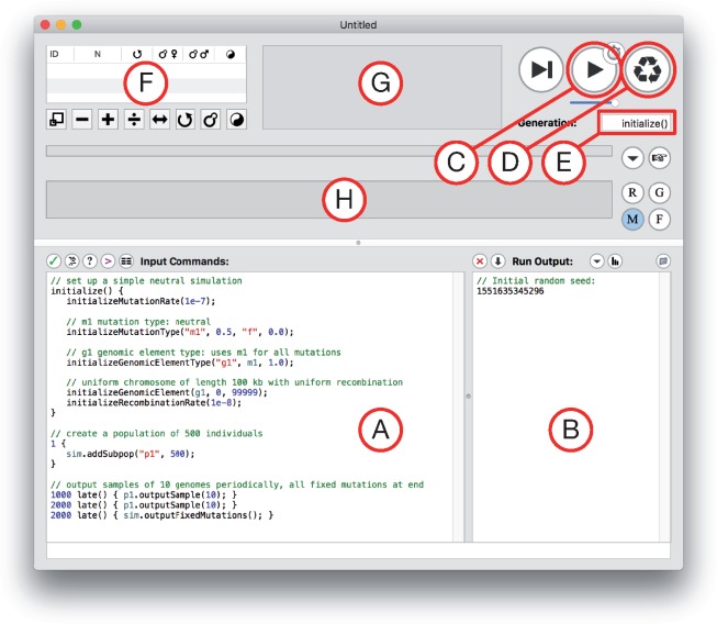
After running the installer, double-click the SLiMgui application to launch it; you should see a new modeling window similar to that shown in fig. 1 (it may not look exactly the same, since there are “splitters” in the SLiMgui window you can move to reveal or conceal various controls). Figure 1 labels various parts of the window, so it is worth studying; some buttons are not labeled there, but if you hover the mouse for a few seconds over the various buttons in this window tooltips will appear explaining what each does.

Fig. 1.

A snapshot of a new modeling window in SLiMgui, with major components labeled by letters. (A) The scripting pane, which contains the script that SLiM will run. (B) The output pane, where text output from the running model appears. (C) The play button, which starts execution of the model in SLiMgui. (D) The recycle button, which resets SLiMgui to use the current model script. (E) The generation counter, which shows the current generation in the simulation. (F) The population view, which lists the subpopulations in the population and shows some of their properties. (G) The individual view, which shows the simulated individuals and their fitness values (indicated by color). (H) The chromosome view, which shows the simulated chromosome across the population, including the frequencies of all mutations.

In SLiMgui, the script is shown in the scripting pane (fig. 1A). Note that SLiMgui’s initial window already contains a default script (fig. 1A); we will not be using that default script, so in each step of this protocol you should select the existing script in the SLiMgui window, delete it, and then type the model code for that step (or, of course, you can create a new modeling window for each step if you wish). The scripts for each step are also available as supplementary text files, Supplementary Material online, with additional comments (supplementary file S1–S3, Supplementary Material online); if you don’t wish to type out each model, those text files can be opened from SLiMgui’s File menu or their text can be pasted into an existing SLiMgui window.

Step 1: A Simple Neutral Model

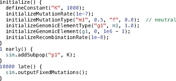
We will begin with a very simple model of a neutral chromosome evolving in a population of 1000 diploid individuals (supplementary file S1, Supplementary Material online); see Code Sample 1.

Code Sample 1

The first thing to discuss about this script is that it is written in a language called Eidos (Haller 2016). Eidos is a very simple language, patterned after R, but should also be easy to learn for users familiar with languages such as Python or C++. This script shows examples of function calls, such as the defineConstant() call, as well as method calls on SLiM objects, such as the sim.addSubpop() call; we will explain those concepts below. Note that each statement in the code ends with a semicolon, “;”, and that blocks of statements are enclosed by braces, “{}”. Code structure in Eidos is expressed with braces, as in R, C, C++, and many other languages; the indentation of the code is purely aesthetic, not syntactically significant as it is in, for example, Python. Comments in Eidos begin with “//”, as with the comment “//neutral”; these are purely for annotation, and are not executed.

The top level of this script defines three callbacks, which are essentially blocks of code defined by the model script that are called internally by SLiM during the execution of the model. Each type of callback in SLiM runs at a particular time in the simulation: once at initialization time for the initialize() callback to set up the initial properties of the model, once at the beginning of generation 1 for the 1 early() event to create the simulated population, and once at the end of generation 10000 for the 10000 late() event to generate final output from the model. (As their names suggest, early() events run early in a specified generation, and late() events run later; precisely when in the generation cycle they run is described in the SLiM manual.) A quick-reference sheet summarizing the basic callbacks used in SLiM is provided in supplementary file S4, Supplementary Material online.

This script creates a subpopulation of K diploid individuals, where K is defined by a defineConstant()function call. A function call tells Eidos to execute a chunk of code to do something useful—in this case, to define a new constant. Defining constants allows fixed parameters of a model to be separated out, making it easy to supply their values on the command line when running the model outside SLiMgui. The addSubpop()method call then uses K as the subpopulation size. Method calls, like function calls, cause a chunk of code to be executed to do something useful, but method calls are associated with a particular target object; the method call queries or modifies the state of the target. The target of the addSubpop() method, named sim, is a global object defined by SLiM that represents the simulation as a whole; the dot operator, “.”, tells Eidos to call the method named addSubpop() on sim to add the new subpopulation to the simulation. The newly created subpopulation is named p1, according to the string name passed to addSubpop(). The new individuals in p1 have empty genomes, with no mutations; they are thus genetically identical and have identical fitness. As the model runs new mutations will arise and will be inherited; mutations can be thought of as changes from the initial empty “wild-type” genomic state.

The rates at which new mutations and recombination crossovers will occur are defined in the initialize() callback. The initializeMutationRate(1e-7) call tells SLiM to generate new mutations during meiosis at a rate of 10⁻⁷ per base position per generation. Similarly, the initializeRecombinationRate(1e-8) call tells SLiM to generate crossover events during meiosis at a rate of 10⁻⁸ per base position per generation. These rates can be modified over time, and regionally varying rate maps along the chromosome may be supplied rather than uniform rates.

The genetic structure for the model is defined by calls to initializeMutationType(), initializeGenomicElementType(), and initializeGenomicElement(). The call to initializeMutationType() defines a new mutation type, m1. Mutation types represent particular classes of mutations used by the model, such as neutral mutations, beneficial mutations, deleterious mutations, or—as we will see in the final model—QTLs. Mutation types are defined primarily by the distribution of fitness effects (DFE) from which mutations of each type are drawn. Here m1 is defined as representing neutral mutations, with a fixed ("f") DFE using a selection coefficient of 0.0 (and a dominance coefficient of 0.5, but that doesn’t matter since the mutations are neutral). The call to initializeGenomicElementType() then defines a new genomic element type, g1. Genomic element types represent particular classes of genomic regions, such as coding and noncoding regions, exons and introns and UTRs, or whatever other sorts of genomic regions are being modeled. Different genomic element types are defined primarily by the mix of mutation types from which new mutations in these elements are drawn; for example, noncoding regions might only undergo neutral mutations, whereas coding regions might also undergo beneficial and deleterious mutations. Here g1 is defined as generating mutations from the mutation type named m1 that was just defined. Finally, the initializeGenomicElement() call tells SLiM that the chromosome contains a genomic element—a genomic region that should be simulated—that is of type g1, beginning at base position 0 and ending at position 10⁶−1 for a total length of 10⁶ base positions. Since this is the only genomic element defined, this element represents the entire simulated chromosome in this model. In short, then, this simple model has a chromosome consisting of a single simulated region, spanning the base interval [0, 10⁶−1], that undergoes only neutral mutations; however, these basic components can be put together in arbitrarily complex ways to represent any genomic structure.

This model generates output at the end of execution using a built-in output method named outputFixedMutations(). As its name suggests, this dumps a list of fixed mutations to SLiM’s output. There are several other built-in output methods, but one may also produce custom output by writing Eidos code, as we will see in the next step.

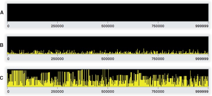
Having discussed the structure of this model, it is now time to run it. Assuming you have the model code above entered in SLiMgui’s scripting pane, you should now click the recycle button (fig. 1D); whenever the script changes and you want to start over from the beginning, you need to recycle to clear the output pane, choose a new random number seed, and reset the simulation. Then click the play button (fig. 1C); this will begin playing the simulation forward in time. As the simulation runs, notice that the simulated subpopulation p1 appears in the population view (fig. 1F); the generation counter (fig. 1E) counts upward; squares representing simulated individuals appear in the individual view (fig. 1G), all colored yellow (indicating that all individuals have the same fitness of one); and the output pane (fig. 1B) displays output when the model finishes at generation 10000. As the simulation runs, the chromosome view (fig. 1H) shows a rapidly changing display of the population frequencies of all of the simulated mutations along the chromosome; fig. 2 shows snapshots of the chromosome view from this model. SLiM generally does not explicitly model the genetic state at every base position (with, e.g., a nucleotide sequence); instead, SLiM only keeps track of the presence of mutations from a base ancestral state. The snapshots in fig. 2 thus illustrate how this model builds up diversity over time from its initially empty (i.e., wild-type or ancestral) state.

Fig. 2.

Snapshots of Step 1’s model running in SLiMgui at the end of generation 1 (A), 500 (B), and 10000 (C). These snapshots of the chromosome view for this neutral model show (A) the empty initial chromosome, (B) the initial establishment of neutral diversity early in the model run, and (C) an equilibrium level of neutral diversity after 10N generations. Each panel shows the simulated chromosome from beginning to end (left to right); each bar represents one mutation, colored yellow (online only) because it is neutral, with a height corresponding to its frequency in the population. Fixed mutations, of which there would be many in panel C, are not shown since by default they are removed from the simulation by SLiM (see text).

All of this is discussed in considerably more detail in the SLiM manual (Haller and Messer 2016); in particular, chapter 1 provides an overview of the conceptual underpinnings of SLiM, and chapter 4 walks through a similar model in great detail.

Step 2: Adding Deleterious and Beneficial Mutations

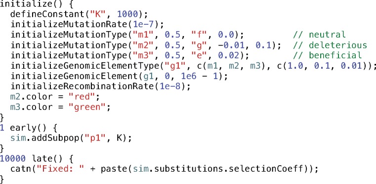
In this step we will make our model nonneutral, adding purifying selection and adaptation through new beneficial mutations. Mutations in SLiM have a selection coefficient that is drawn from the distribution of fitness effects (DFE) of their mutation type. So far, we have modeled neutral mutations with a selection coefficient of 0.0; we will now add two new mutation types, representing deleterious and beneficial mutations (supplementary file S2, Supplementary Material online) (Code Sample 2).

Code Sample 2

There are several changes here from the previous step. In the initialize() callback we now make three calls to initializeMutationType(), creating three different mutation types. The first, m1, is unchanged, using a fixed ("f") DFE with a selection coefficient of 0.0. The second, m2, uses a gamma ("g") DFE to represent deleterious mutations, with a mean selection coefficient of -0.01 and a shape parameter of 0.1. The third, m3, uses an exponential ("e") DFE to represent beneficial mutations, with a mean selection coefficient of 0.02. These choices are fairly arbitrary, but illustrate that various kinds of DFE are supported by SLiM.

Having set up these mutation types, initializeGenomicElementType() now defines genomic element type g1 as representing genomic regions that undergo all three types of mutations, as expressed by c(m1, m2, m3); the c() function sticks its parameters together, allowing all three mutation types to be passed together to initializeGenomicElementType() as a single parameter. The next parameter, c(1.0, 0.1, 0.01), tells SLiM that new mutations of these mutation types should occur at the given relative frequencies; for every one m1 mutation there will be, on average, 0.1 deleterious m2 mutations and 0.01 beneficial m3 mutations.

At the end of the initialize() callback we tell SLiMgui to display m2 mutations in red and m3 mutations in green by setting the color property of the mutation types. This is the first time we have used properties in Eidos; they are just little bits of information attached to objects that can be accessed and set using the dot operator, “.”, similarly to how the dot operator is used to call methods on an object. The properties and methods defined for SLiM’s objects in Eidos are documented in the SLiM manual (Haller and Messer 2016). Note that the color names "red" and "green", and many others, are predefined by Eidos following the named colors in R.

The other change in this step is that the outputFixedMutations() call has been replaced by some customized output. Here, we call the catn() function to concatenate output to the Eidos output stream, followed by a newline (the “n” in catn()). The output consists of a string, "Fixed: ", followed by the selection coefficients of all fixed mutations, pasted together into a big string by paste(). Those selection coefficients are obtained through properties, but how exactly that works needs a little discussion.

First of all, SLiM turns fixed mutations into substitution objects, by default. This is because fixed mutations generally do not affect evolutionary dynamics; since every individual carries them, they produce no fitness differences between individuals, and can thus be ignored. This is not always true (epistasis, in particular, violates this assumption), and so this default behavior can be changed; but usually it is true, and so SLiM assumes it as the default to allow models to run more efficiently. The substitutions property of sim provides a vector of these substitution objects, representing the mutations that have fixed in the population. A vector, in this sense, is simply a collection of zero or more values of a particular type; one can speak of a vector of integers or a vector of objects. Eidos, like R, is a vector-based language; in Eidos, a single line of vectorized code often does what an entire for loop would do in other languages, allowing Eidos to be relatively fast even though it is an interpreted language. We actually used vectors before, when we called c(m1, m2, m3) and c(1.0, 0.1, 0.01); the c() function creates a vector out of the values it is passed. In fact, we have been using vectors all along; everything in Eidos is a vector, even single values like 1.0 or sim, because single values are just vectors that happen to contain exactly one element (called singletons in Eidos parlance). So, sim.substitutions provides a vector containing all of the substitutions in the simulation. We then chain an access of the selectionCoeff property onto that; this is a vectorized property access, fetching the value of the selectionCoeff property from each substitution object in the target vector. The result is a new vector that contains the selection coefficients of all of the substitutions; the paste() function then turns that vector into a single string for output.

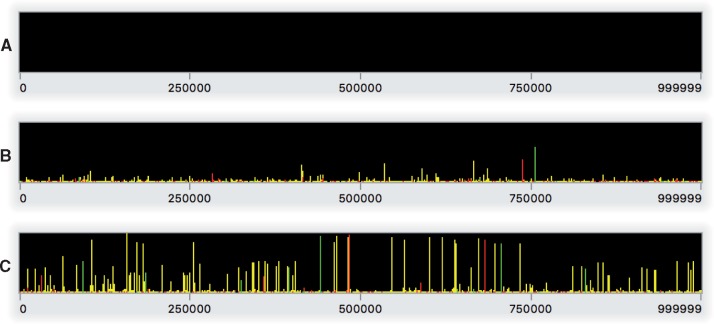
Running this model in SLiMgui (do not forget to recycle before clicking play) produces a series of sweeps by beneficial mutations, often with deleterious and neutral mutations carried along by hitchhiking; fig. 3 shows snapshots of the chromosome view from a typical run of the model. Notice that given the specification of the genetic architecture in the initialize() callback—mutation types, genomic element types, genomic elements, etc.—all of the model dynamics are handled automatically by SLiM. There is no need to write any code to explicitly manage fitness or selection in the model, and indeed the script contains no code whatsoever stating what should happen in any generation from 2 to 9999; SLiM’s default behavior is automatic. In the next step, however, since we will modify some of SLiM’s default behavior, we will need to write a little bit of code to explicitly influence fitness in each generation.

Fig. 3.

Snapshots of Step 2’s model running in SLiMgui at the end of generation 1 (A), 200 (B), and 10000 (C). These snapshots of the chromosome view for this nonneutral model show (A) the empty initial chromosome, (B) early in the run with a sweeping beneficial mutation (green bar) and a deleterious mutation that is hitchhiking nearby (red bar), along with some neutral diversity (yellow bars) and low-frequency nonneutral mutations, and (C) the model after 10N generations, with a variety of beneficial, deleterious, and neutral mutations at various frequencies. Fixed mutations, of which there would be many in panel C, are again not shown.

Step 3: Adding QTLs and Selection on Phenotype

In the previous step we modeled beneficial and deleterious mutations. The fitness of an individual was determined by the selection coefficients of all mutations it carried in its genomes (SLiM assumes multiplicative effects across individual loci by default). In this step, we will adapt that script to instead model mutations that represent quantitative trait loci (QTLs): the mutations will affect the phenotype of an individual in an additive fashion, and each individual’s fitness will be based on its phenotype, rather than the selection coefficients of the QTL mutations. The same QTL mutation might therefore be beneficial or deleterious, depending upon the genetic background in which it occurs and the overall phenotype generated by the additive effects of all of the QTLs possessed by an individual.

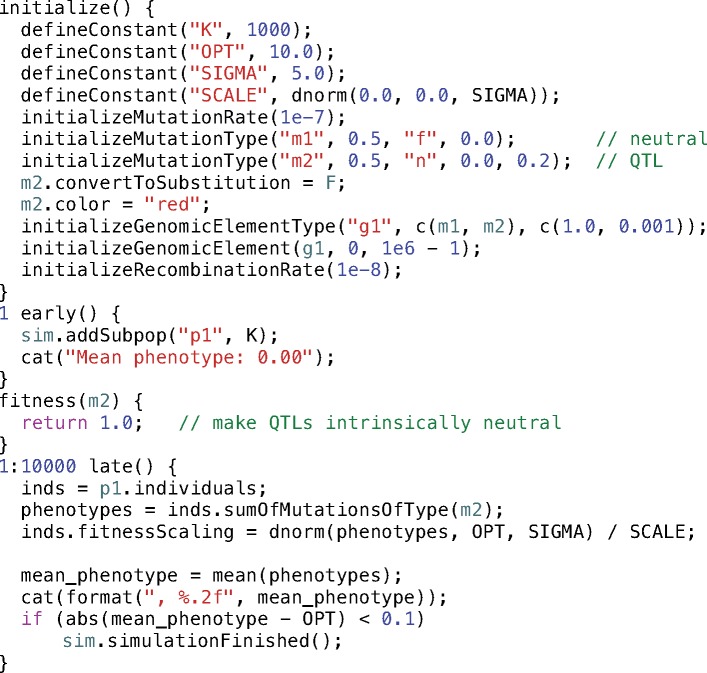
To implement this in SLiM, we will alter SLiM’s default behavior in a few key ways in the model’s script. The core idea is that we will repurpose the selection coefficients of m2 mutations to represent QTL effect sizes instead. Normally, SLiM uses the selection coefficients of mutations to multiplicatively compute individual fitness values; but here we will tell SLiM to consider m2 mutations neutral (ignoring their selection coefficients), and we will implement our own fitness-calculation machinery that uses the values stored in the selection coefficient property as additive QTL effect sizes instead. The resulting script (supplementary file S3, Supplementary Material online) is shown in Code Sample 3.

Code Sample 3

The initialize() callback defines a few new constants (OPT, SIGMA, and SCALE) related to the phenotypic fitness function that we will define later. It sets up a neutral mutation type m1 as before, but also creates an m2 mutation type to represent QTLs. The m2 mutation type draws mutation effect sizes from a DFE specified by a normal (Gaussian) distribution (type "n") with mean 0.0 and standard deviation 0.2. As mentioned before, by default SLiM would remove mutations from the simulation if they become fixed in the population; here, however, we want QTL mutations to be kept even when they have fixed, since they will continue to influence fitness through their effect on phenotype, so we set the convertToSubstitution property of m2 to F (false). We also configure m2 to display in red in SLiMgui, for visibility. Finally, we tell SLiM that genomic element type g1 should undergo both m1 and m2 mutations, in relative proportions of 1.0 and 0.001; this gives us a mostly neutral model with occasional QTL mutations.

The configuration of m2 makes all new mutations of type m2 have selection coefficients drawn from the specified normal distribution. This is not quite what we want, however; we want m2 mutations to be intrinsically neutral, as far as SLiM’s built-in fitness-calculation machinery is concerned, since we want to use those values to additively compute phenotypes instead. To achieve this, we define a new type of callback, the fitness(m2) callback. The fitness() callback mechanism allows the fitness effect of mutations of a given type to be redefined; SLiM will call a fitness() callback for every mutation of its given type, in every generation, in every individual, allowing fitness effects to vary over time or between individuals. Here we simply return a fitness effect of 1.0, making m2 mutations neutral. With this callback, QTL mutations will still have “selection coefficient” values drawn from the specified normal distribution, but they will be considered neutral by SLiM’s fitness-calculation machinery. We will instead use the selection coefficient values of the QTL mutations as phenotypic effect sizes, as described below.

The final step to implement this model of QTL evolution is the 1:10000 late() event (in Eidos the colon operator, “:”, computes a range of values, so 1:10000 tells SLiM to run this event every generation from 1 to 10000). The first line fetches the individuals property from p1 (our subpopulation object); this yields a vector of the individuals in p1, which is assigned to a new variable, inds (variables are essentially just symbolic names for values). Next we call sumOfMutationsOfType(m2) on inds; this is a vectorized method call, similar to the vectorized property access we saw earlier. It returns a new vector, with one element per individual, containing the sum of the selection coefficients of m2 mutations in each individual (across both genomes); these sums are the phenotypes of the individuals, calculated additively from the effect sizes of all QTLs possessed by each individual. The result is placed in a new variable named phenotypes. The next line, which calculates fitness effects due to phenotype, is also vectorized: the dnorm() function calculates, for each phenotypic value in the phenotypes vector, the probability density for a normal distribution centered at OPT, with a standard deviation of SIGMA, and returns a vector of fitness effects which are then normalized by dividing them by the maximum density, SCALE. These fitness effects are assigned, again in a vectorized fashion, to the fitnessScaling property of the individuals in inds; each individual is given its corresponding fitness effect by the vectorized property assignment. These fitnessScaling values modify the fitness of individuals based on their phenotype, because SLiM multiplicatively combines the fitnessScaling values of individuals with any other fitness effects in the model to produce final fitness values. The dnorm() function here thus describes the phenotypic fitness function for the model: a Gaussian function with a width of SIGMA that determines the strength of selection, and a fitness optimum at OPT.

In the second part of the 1:10000 late() event, we calculate the mean phenotype across the subpopulation using mean() and concatenate it to SLiM’s output with cat() (like catn(), but without a newline added at the end). Together with the initial cat() call in the 1 early() event, this will output a comma-separated sequence of the mean phenotype from each generation. This provides another example of custom output using Eidos, here produced generation by generation rather than in a single output event. Finally, we check whether the mean phenotype is within a tolerance of 0.1 of the phenotypic optimum, OPT; if it is, the adaptive walk to the optimum is deemed complete, and we end the simulation with a call to sim.simulationFinished().

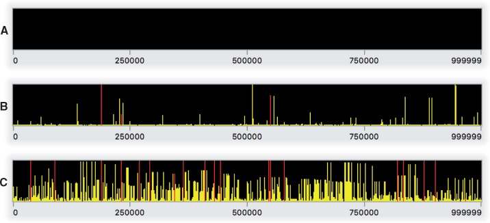
Figure 4 shows snapshots of the chromosome view of this model as it runs in SLiMgui. Here QTL mutations, shown in red, have arisen at several random locations along the chromosome, and their additive effects have produced adaptation to the fitness optimum by the end of the adaptive walk. In this model, new QTLs arise randomly through mutation at any genomic locus; it would be straightforward to define a genetic structure in which QTLs exist only at predefined loci in the genome using different genomic elements, genomic element types, and mutation types. It would also be simple to start the model with some QTL mutations already present in some or all individuals, by adding QTL mutations to the genomes of the initial generation as desired; one could thus model evolution from a particular pattern of standing genetic variation in a trait.

Fig. 4.

Snapshots of Step 3’s model running in SLiMgui at the end of generation 1 (A), 200 (B), and 5652 (C). These snapshots of the chromosome view for this QTL-based model show (A) the empty initial chromosome, (B) a fixed QTL and another QTL in mid-sweep (red bars) with reduced and skewed neutral diversity due to those sweeps, and (C) the state of the model after completion of an adaptive walk to the optimum, with 14 fixed or high-frequency QTLs.

Discussion

We have shown how to build a simple SLiM model from scratch, providing a step-by-step introduction to the SLiM framework for new users. The final model we built involved the evolution of a polygenic quantitative trait modeled with QTLs that additively produce a selected phenotype, but the lessons learned should be general to all SLiM models.

Importantly, we have shown several screenshots from SLiMgui to leverage the power of interactive, graphical model development. SLiMgui has built-in help for Eidos and SLiM (hold down the option key and click on any property name, method name, or keyword). It provides code completion to speed up typing (press escape while typing to see possible completions for a prefix you have typed). It also provides graphs of various simulation metrics, a built-in Eidos console for interactive scripting while a simulation is running, performance profiling to find the “hot spots” in a model’s code, and much more. SLiMgui is not just a code editor, it is a full-featured modeling environment, and a key part of SLiM for beginners and advanced users alike.

The SLiM manual (Haller and Messer 2016) has over 100 different “recipes” for models of all sorts, from simulating human evolutionary history to simulating a CRISPR gene drive; one can create models of discrete subpopulations connected by migration or models of subpopulations dispersing across continuous spatial landscapes, models of cloning or selfing or haploids with horizontal gene transfer, models with balancing or frequency-dependent or temporally varying selection, models of selective sweeps or assortative mating or social learning, models of extinction-colonization dynamics or pollen flow or habitat choice—the scriptability of SLiM provides tremendous flexibility. However, the basic concepts discussed in this article apply to all SLiM models, so let us review them in conclusion.

One general concept regards the way SLiM defines the genetic structure of organisms, with individuals containing genomes that contain mutations defined by their mutation type, and a chromosome composed of genomic elements defined by their genomic element type. This structure is the same in every SLiM model, but it can be made arbitrarily complex. It is straightforward to build SLiM models of realistic genetic structure such as introns and exons and UTRs; indeed, one can represent the entire genetic map of a model organism such as Drosophila in SLiM.

Another general concept regards the initialize() and fitness() callbacks, and early() and late() events, that we saw here; these hooks for modifying SLiM’s default behavior prove useful in a wide variety of contexts. SLiM provides several more callback types, such as mateChoice(), modifyChild(), and reproduction() callbacks, for customizing other aspects of model behavior.

A final general concept is the Eidos scripting language itself, since it is the foundation of all SLiM models. To take full advantage of SLiM’s capabilities, it is important to learn Eidos properly. Eidos provides dozens of useful functions, often based upon R functions of the same name; they are all documented in the Eidos manual (Haller 2016). More fundamentally, it is important to embrace the vectorized philosophy of Eidos; if you find yourself writing a for loop, ask yourself whether the code could be vectorized instead (note that the models shown here do not use a single loop).

SLiM 3 is free, licensed under the GNU GPL, and is open source on GitHub. The latest version of SLiM, including manuals and quick-reference sheets, is available from https://messerlab.org/slim/. We also recommend that new SLiM users subscribe to the slim-discuss mailing list at http://bit.ly/slim-discuss. The learning curve for SLiM can be steep, but we hope that this protocol, and the resources we have cited here, will help introduce a new generation of users to the power, flexibility, and speed of SLiM.

References

- Bank C, Ewing GB, Ferrer-Admettla A, Foll M, Jensen JD. 2014. Thinking too positive? Revisiting current methods of population genetic selection inference. Trends Genet. 30(12):540–546. [DOI] [PubMed] [Google Scholar]
- Carvajal-Rodriguez A. 2010. Simulation of genes and genomes forward in time. Curr Genomics. 11(1):58–61. [DOI] [PMC free article] [PubMed] [Google Scholar]
- Champer J, Zhao J, Champer S, Liu J, Messer PW. 2018. Population dynamics of underdominance gene drive systems in continuous space. bioRxiv 449355, 10.1101/449355. [DOI] [PMC free article] [PubMed]
- Fijarczyk A, Dudek K, Niedzicka M, Babik W. 2018. Balancing selection and introgression of newt immune-response genes. Proc R Soc B. 285:1–9. [DOI] [PMC free article] [PubMed] [Google Scholar]
- Grimm V. 2002. Visual debugging: a way of analyzing, understanding and communicating bottom-up simulation models in ecology. Nat Resour Model. 15(1):23–38. [Google Scholar]
- Haller BC. 2016. Eidos: a simple scripting language. Available from: http://benhaller.com/slim/Eidos_Manual.pdf.
- Haller BC, Galloway J, Kelleher J, Messer PW, Ralph PL. 2019. Tree-sequence recording in SLiM opens new horizons for forward-time simulation of whole genomes. Mol Ecol Resour. 19(2):552–566. [DOI] [PMC free article] [PubMed]
- Haller BC, Messer PW. 2016. SLiM: an evolutionary simulation framework. Available from: http://benhaller.com/slim/SLiM_Manual.pdf.
- Haller BC, Messer PW. 2017a. SLiM 2: flexible, interactive forward genetic simulations. Mol Biol Evol. 34(1):230–240. [DOI] [PubMed] [Google Scholar]
- Haller BC, Messer PW. 2017b. asymptoticMK: a web-based tool for the asymptotic McDonald–Kreitman test. G3 7(5):1569–1575. [DOI] [PMC free article] [PubMed] [Google Scholar]
- Haller BC, Messer PW. 2018. SLiM 3: forward genetic simulations beyond the Wright–Fisher model. Mol Biol Evol. 36(3):632–637. [DOI] [PMC free article] [PubMed]
- Henden L, Lee S, Mueller I, Barry A, Bahlo M. 2018. Identity-by-descent analyses for measuring population dynamics and selection in recombining pathogens. PLoS Genet. 14(5):e1007279. [DOI] [PMC free article] [PubMed] [Google Scholar]
- Hoban S. 2014. An overview of the utility of population simulation software in molecular ecology. Mol Ecol. 23(10):2383–2401. [DOI] [PubMed] [Google Scholar]
- Kim BY, Huber CD, Lohmueller KE. 2018. Deleterious variation shapes the genomic landscape of introgression. PLoS Genet. 14:1–30. [DOI] [PMC free article] [PubMed] [Google Scholar]
- Kosheleva K, Desai MM. 2018. Recombination alters the dynamics of adaptation on standing variation in laboratory yeast populations. Mol Biol Evol. 35(1):180–201. [DOI] [PMC free article] [PubMed] [Google Scholar]
- Librado P, Orlando L. 2018. Detecting signatures of positive selection along defined branches of a population tree using LSD. Mol Biol Evol. 35(6):1520–1535. [DOI] [PMC free article] [PubMed] [Google Scholar]
- Matz MV, Treml EA, Aglyamova GV, Bay LK. 2018. Potential and limits for rapid genetic adaptation to warming in a Great Barrier Reef coral. PLoS Genet. 14(4):e1007220. [DOI] [PMC free article] [PubMed] [Google Scholar]
- Messer PW. 2013. SLiM: simulating evolution with selection and linkage. Genetics 194(4):1037–1039. [DOI] [PMC free article] [PubMed] [Google Scholar]
- Nowak MD, Haller BC, Yoder AD. 2014. The founding of Mauritian endemic coffee trees by a synchronous long-distance dispersal event. J Evol Biol. 27(6):1229–1239. [DOI] [PubMed] [Google Scholar]
- Parada JLC, Charlesworth B. 2018. The effects on neutral variability of recurrent selective sweeps and background selection. bioRxiv 358309, 10.1101/358309. [DOI] [PMC free article] [PubMed]
- Pouyet F, Aeschbacher S, Thiéry A, Excoffier L. 2018. Background selection and biased gene conversion affect more than 95% of the human genome and bias demographic inferences. Elife 7:e36317. [DOI] [PMC free article] [PubMed] [Google Scholar]
- Rougemont Q, Carrier A, Leluyer J, Ferchaud A-L, Farrell J, Hatin D, Brodeur P, Bernatchez L. 2018. Combining population genomics and forward simulations to investigate stocking impacts: a case study of Muskellunge (Esox masquinongy) from the St. Lawrence River basin. Evolutionary Applications, Advance Access, 10.1111/eva.12765. [DOI] [PMC free article] [PubMed]
- Thornton KR. 2014. A C++ template library for efficient forward-time population genetic simulation of large populations. Genetics 198(1):157–166. [DOI] [PMC free article] [PubMed] [Google Scholar]
- Yuan X, Miller DJ, Zhang J, Herrington D, Wang Y. 2012. An overview of population genetic data simulation. J Comput Biol. 19(1):42–54. [DOI] [PMC free article] [PubMed] [Google Scholar]
Associated Data
This section collects any data citations, data availability statements, or supplementary materials included in this article.