Abstract
Repeat Image Feature Tracking (RIFT) is commonly used to measure glacier surface motion from pairs of images, most often utilizing normalized cross correlation (NCC). The Multiple-Image Multiple-Chip (MIMC) algorithm successfully employed redundant matching (i.e. repeating the matching process over each area using varying combinations of settings) to increase the matching success rate. Due to the large number of repeat calculations, however, the original MIMC algorithm was slow and still prone to failure in areas of high shearing flow. Here we present several major updates to the MIMC algorithm that increase both speed and matching success rate. First, we include additional redundant measurements by swapping the image order and matching direction; a process we term Quadramatching. Second, we utilize a priori ice velocity information to confine the NCC search space through a system we term dynamic linear constraint (DLC), which substantially reduces the computation time and increases the rate of successful matches. Additionally, we develop a novel post-processing algorithm, pseudosmoothing, to determine the most probable displacement. Our tests reveal the complimentary and multiplicative nature of these upgrades in their improvement in overall MIMC performance.
Keywords: Image matching, Image motion analysis, Velocity measurement
I. Introduction
Due to the expanse and remoteness of glaciers and ice sheets, airborne and satellite remote sensing provide the only practical means for mapping ice motion over large areas and at frequent time intervals. Combined Synthetic Aperture Radar Interferometry (InSAR) and speckle tracking ([1]) have been the primary tool for constructing ice velocity maps over large areas and nearly complete coverage for Greenland and Antarctic Ice Sheet is available for multiple epochs (e.g. [2], and [3]). These data, however, are limited in temporal resolution and range, hampering studies of seasonal or interannual glacier change over many years. On the other hand, Repeat-Image Feature Tracking (RIFT) can be applied to any pair of coregistered images, including nearly five decades of Landsat satellite imagery openly distributed by the United States Geological Survey (USGS) Landsat open archive and, beginning in 2014, the European Space Agency’s Sentinel constellation of both SAR and optical imagery. RIFT has been used to reconstruct short-term variability in glacier motion and mass balance in a number of studies (e.g., [4]–[8]) Additionally, the Optical Land Imager (OLI) aboard Landsat 8, launched in 2013, offers enhanced RIFT capabilities for glaciers and ice sheets through both increased radiometric resolution and higher signal-to-noise ratio ([9], and [10]).
In order to generate wide-area maps of glacier motion at frequent time intervals using RIFT, several challenges must be overcome. Firstly, the RIFT algorithm must be general enough to track features over a range of displacements and not be sensitive to parameters such as search window size. Secondly, the algorithm must be able to properly handle image errors, including the null striping found in Landsat 7 Enhanced Thematic Mapper Plus (ETM+) resulting from failure of the Scan-Line Corrector (termed, SLC-off imagery). Third, the algorithm needs to mitigate unfavorable atmospheric conditions, such as haze and cloud cover in optical images, which can cause spurious matches. Last, the algorithm must be efficient to process large numbers of pairs at minimal computational cost.
To address the above issues, [11] developed a RIFT approach, called Multi-Image, Multi-Chip (MIMC), in which features are tracked through Normalized Cross-Correlation (NCC) using a range of search and reference window sizes and multiple convolution filters. The displacement for each tracked pixel is then determined from the population of individual measurements, termed the “voting cell” method. The MIMC approach is based on the assumption that increasing the number of matching attempts using different matching settings (search and reference window sizes and image enhancements) increases the probability of a successful match. This effectively generalized the RIFT method, but had a high computational cost due to the number of individual searches performed. In addition to the multiple matching attempts, the algorithm also mitigated the effect of the SLC-off voids by calculating the NCC in the spatial, rather than frequency, domain, further reducing computational efficiency ([6], [11]–[13]). This was improved by [12] who used NCC-based RIFT in the frequency domain by filling the null gaps with values that did not influence the NCC calculation in frequency domain.
While MIMC and other RIFT algorithms typically use only forward matching (i.e. the first image always provides the reference chip and the second image always provides the search chip) for NCC calculations, [14] proposed reversing the image order to utilize the “reverse correlation” results for finding correct matches. Based on this approach, we present an iterative procedure, termed quadramatching (QM) that further increases the matching redundancy and robustness of the statistics of the solutions.
To mitigate increased number of calculations needed for QM, we additionally introduce a Dynamic Linear Constraint (DLC) on the matching procedure based on an a priori velocity field. It is now common for at least one, high-quality map of flow velocity to be available for a given region of interest for large ice sheets such as Greenland or Antarctica (e.g. [2], and [3]). In case that an existing velocity map is not available, a velocity map derived from another image pair in a time series of images can play role as a priori. These data constrain the RIFT search parameters and range, which can increase the computational efficiency and reduce the number of spurious matches. This increase in computational efficiency can then enable additional steps to improve the generality of the algorithm and accuracy of the results.
Here we present substantial improvements in efficiency and effectiveness to an NCC-based RIFT algorithm applied to glacier flow. Our updates are intended to provide robust, fast and automated processing of large numbers of image pairs over areas of complex flow, such as shear margins and calving fronts.
II. Method and Data
A. Quadramatching
Our algorithm builds upon the redundant solution approach of Multi-Image Multi-Chip (MIMC) RIFT method presented in [11] with the addition of iterative forward and reverse matching that we term Quadramatching (QM). A study in [14] proposed adding a redundancy to the match solution by swapping the reference and search chips from the initial, “forward” match and using these to solve for an additional “reverse” match. In the study, the closer the solutions of the forward and reverse matches, the greater the confidence of the displacement solution.
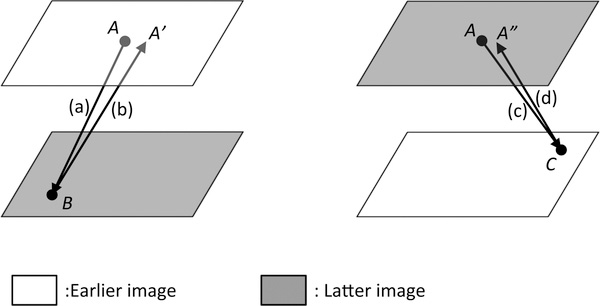
For the QM approach, we obtain further redundancy in the match solution by iteratively reversing both the direction of the search and the order of the image pair (pair swapping), resulting in four solutions that are combined to provide the match location and confidence. The QM procedure is illustrated in Fig.1. Initially, point A on the first image (I0) is matched to point B on the second image (I1). A new reference chip is the extracted around point B on I1, and the search is repeated on I0, giving the backwards match to point A’. This location is referred to as the “original pairing” result. Next, the order of images I0 and I1 are reversed and the forward-backward search procedure is repeated, giving the “swapped pairing” match at location A”.
Fig.1.
Schematic illustration of quadramatching, (a): Original forward, (b): Original backward, (c): Swapped original, (d): Swapped backward.
Although those four sets of measurements are from the same image pair, they are not identical measurements. The differences between the solutions can be identified by first defining the initial match (forward matching from the original pairing) as:
| (1) |
where the first and the second arguments on the left side are the reference chip and the search window (i.e. image to find the matching point). The superscript indicates the coordinates of the image chip and the subscript is the source of the image chip or the search window (0 is the earlier, 1 is the latter). Thus, (1) states that the original forward solution, point B in I1, is determined from a reference chip around point A in I0 and a search chip in I1. In the same convention, the three other matches are described as:
| (2) |
| (3) |
| (4) |
Since each match solution has a different reference chip , they yield displacement vectors with different origins. Respectively, their displacements are:
| (5) |
| (6) |
| (7) |
| (8) |
with subscripts O, S, F, and B for original pair, swapped pair, forward match, and backwards match, respectively. This procedure is applied to each set of chip size and filter combinations in MIMC, thus increasing the number of displacement solutions by a factor of four.
B. Dynamic Linear Constraint
Glacier speed can change abruptly in response to stress perturbations caused by, for example, calving front retreat and variations in basal water pressure. Measurement of these speed variations is a typical objective for RIFT applications. The direction of flow, however, tends to remain relatively constant through time; since direction is primarily determined by the surface slope and large variations in flow direction that would require large changes in the ice thickness field. Therefore, if the direction of flow is known from an existing velocity map, or can be estimated from a digital elevation model or numerical ice flow model, it can be used to both constrain the area of NCC matching and to prevent spurious matches without biasing the measurement result. Examples of this approach include [14] and [15] that made use of existing ice flow measurements as a priori information to limit the location of the matching solution to within a defined rectangular boundary. Another major advantage of using such a directional constraint on the match solution is the large reduction in the number of NCC computations per match area. This is especially important when utilizing redundant match approaches such as MIMC and QM.
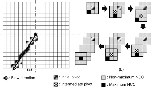
A concern in the use of an existing velocity field as a priori information for constraining the matching procedure is that errors in that velocity field, or change in surface flow between the times when the a priori field was constructed and the imagery to be used for RIFT was obtained, could influence the result, reducing the accuracy of the solution. To mitigate this effect, we use a non-deterministic approach, illustrated in Fig.2, to constrain the search for the NCC peak within the matching procedure. First, the a priori displacement vector, starting at the reference origin, is projected onto the search image and the pixels that intersect this vector are chosen as initial “pivots” from where the NCC peak search begins. For each initial pivot pixel, the NCC field is calculated for the search image chip centered on the pivot and the 8 surrounding pixels. The location of the maximum NCC value among these 9 solutions is chosen as the new “intermediate” pivot point for the next iteration. The NCC fields for this intermediate pivot and the surrounding pixels are calculated so that the pivot at the next stage is the location of the maximum NCC among the series. The procedure is then repeated until the point of maximum NCC is the intermediate pivot itself (the center of the 3-by-3 cell) so that there is no update in the pivot location. This iteration is then repeated for all initial pivots.
Fig.2.
Normalized cross correlation peak searching algorithm using dynamic linear constraint, (a): Initial pivots lie under the extent of flow vector, (b): iterative searching for the cross correlation peak.
This procedure ensures that each iteration, starting from initial pivot, will converge to a local maximum in NCC space only within or near the known direction of flow. Moreover, by constraining the search area to approximate a vector, the number of NCC calculations is drastically reduced. The length of the vector of initial pivot points is bounded by the magnitude of the expected maximum displacement and the coregistration error. Here, the extent of each search grid (Li,j) was determined by:
| (9) |
where s is a scale factor (chosen to 1.8 in this study based on the maximum expected fluctuation of the flow speed for the test glaciers), vi,j is velocity (unit: m/yr), r is spatial resolution of the image, t is the length of temporal baseline of a pair (unit: day) and c is the maximum expected image coregistration error. Increasing s and/or c reduces the linear constraint, allowing for more deviation in flow direction but increasing the processing time.
C. Postprocessing
A critical postprocessing step of any redundant match approach such as MIMC and QM is the selection of the best single displacement from the population of redundant matches that will nearly always contain spurious single solutions. Several filtering approaches for single matching displacements exist in the literature. They include utilization of the images’ signal-to-noise ratio (SNR) and NCC values ([16]), the SNR of measurements ([17]), forward and backward matching ([14]), expected speed or thresholding based on smooth changes ([1], and [18]), or combinations of these ([19], and [20]). Among those methods, the strain rate approach is based on the assumption that the glacier’s gradient of motion is smooth according to its viscoelastic flow. It has been widely adopted in filtering or postprocessing algorithms. However, strain rate-based filters tend to fail where similar spurious matches are spatially clustered, as typical for errors induced by clouds and shadows.
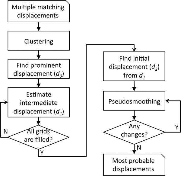
Here, we present a novel post-processing method, termed pseudosmoothing, which determines the most probable displacement from a population of redundant matches (Fig.3). Similar to the “voting cell” method in MIMC ([11]), pseudosmoothing is applied to clusters of multiple matching results (i.e. reference chip size, image filter, and QM) in each of the single grid. We apply a connectivity-based clustering algorithm rather than clustering the displacements into discrete cells as in the voting cell method. If the minimum Euclidian difference between the displacement di and elements in a cluster Ck is less than a threshold value, ρmin, the displacement di is considered as a member of Ck. This criterion for the cluster Ck can be formularized as:
| (10) |
where the distance between the displacement and clusters are:
| (11) |
therefore, for any clusters Ck and Cl,
| (12) |
where
| (13) |
Fig.3.
Postprocessing flow.
We use Ck of 10 and a ρmin of 1 pixel. Next, clusters of displacements are defined. A cluster is considered prominent if its number of samples is more than 60% of the total population. The mean displacement of the prominent cluster is considered the prominent displacement (d0) in the corresponding grid. However, due to the possibility of increased spurious matching, not all grid points have a prominent cluster and corresponding d0s. For those locations, an intermediate displacement (d1) is estimated instead.
The estimation of an intermediate displacement starts from finding the expected displacements (de) based on the given a priori velocity information. The expected displacement is obtained from:
| (14) |
with the same variables as (9). The difference in definitions of coordinate system between a priori and the image may require reversing the coordinate axes. When using a priori values for this calculation, seasonal and annual variability in flow speed should be considered. Therefore, a scale factor needs to be applied to de to compensate the variability. This factor is calculated by comparing de with the neighboring prominent displacements (d0) or d1 in the earlier iterations. When there are a sufficient number of d0 or d1 values around the location (i, j), d1 in the current iteration is calculated as
| (15) |
where the hat denotes the averaged values in the neighbor of (i, j). This iteration is repeated until all grids are filled with either d0 or d1.
Equations (14) and (15) imply that d1 at point (i, j) is not determined from the clustered displacements of the grid point, but from the neighboring d0 or d1 and the a priori displacement. The mean value of the closest cluster to d1 for each grid point, therefore, is chosen as the initial displacement (d2). In this way, the displacement at each grid point is determined from the mean values of grid clusters, which are either d0 or d2.
The resulting d2 is then adjusted through iterative and anisotropic weighted quadratic fitting. For a location (i, j), the displacements (d2) of the neighboring grid points are weighted using a negative exponential function with respect to distance and flow direction. To accommodate large lateral gradients (i.e. shear strains) in glacier flow, the neighboring displacements along the flow direction are given a greater weight than those in the across-flow direction. We term this postprocessing method “pseudosmoothing” because it finds a cluster’s displacement close to the smooth value, but the resultant displacement is neither interpolated nor an average.
D. Procedure
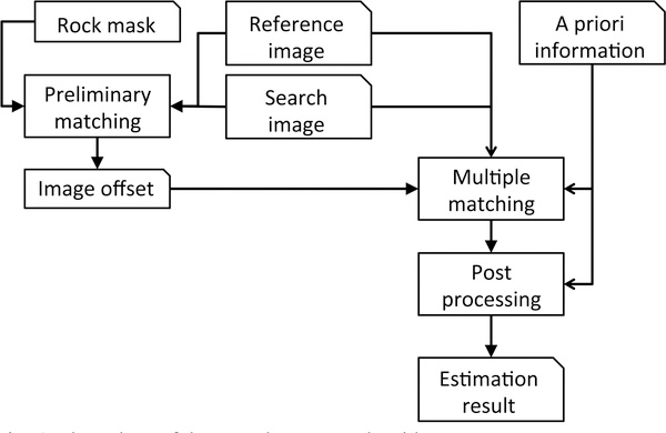
The complete RIFT processing flow is illustrated in Fig.4. A preliminary matching is performed on the image pair to estimate the coregistration error from the offset on stationary (i.e. exposed rock) areas, as defined by a land classification mask. The preliminary matching does not use the DLC because a priori velocity information on stationary areas are not meaningful, since offsets are caused by misalignment in orthorectification process and not by flow. The results obtained from the preliminary matching are clustered using the algorithm described in section II-C and only prominent displacements (mean value of the displacements in the prominent cluster) are chosen to calculate the offset.
Fig. 4.
Flow chart of the complete RIFT algorithm.
Following the RIFT process for coregistration error, the RIFT process is repeated over ice-covered areas using DLC (section II-B). The solutions are then postprocessed as described in section II-C.
E. Test Data and Methods
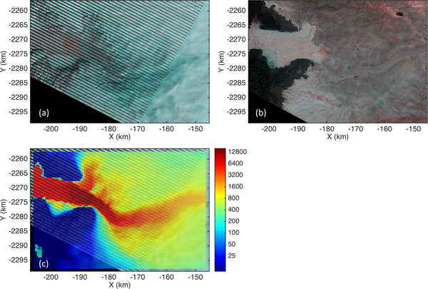
We test our RIFT algorithm using a series of Landsat 7 and 8 panchromatic band images of Jakobshavn Isbræ located on the west coast of Greenland. The site is located at approximately 69° 11’ north and 49° 40’ west. The image pairs were clipped from the full Landsat image tiles and resampled to a polar stereographic projection to match the a priori velocity map, described below. The image pairs are listed in Table I and the anaglyphic composition of the image pairs in Fig.5(a)–(c). Fig.5(a) shows an example of Landsat 7 ETM+ imagery with void stripping from SLC failure and small clouds that would be expected to give poor results. This scenario is chosen to provide a basis of comparison for later results.
Table I.
Test Data
| Pair | Sensor | Acquisition time | Path/Row | Scene ID |
|---|---|---|---|---|
| 1st | ETM+ | April 1,2009 | 8/11 | LE70080112009091EDC00 |
| ETM+ | April 17, 2009 | 8/11 | LE70080112009107EDC00 | |
| 2nd | OLI | July 12, 2014 | 8/11 | LC80080112014193LGN01 |
| OLI | July 28, 2014 | 8/11 | LC80080112014209LGN00 | |
Fig.5.
Anaglyphic color images of the test pairs and reference velocity information, (a): ETM+ image pair of 1 April 2009 and 17 Apr 2009, (b) OLI image pair of 12 July 2014 and 28 July 2014, (c) interpolated InSAR velocity map as a priori data, color-coded in unit of m/yr, with 5(a) in its background. The earlier image in each tested pairs is colored in red, while the latter one is in cyan.
We processed these data with several different scenarios to examine the effect of the individual components (i.e. QM and DLC) of our algorithm on RIFT. Firstly, four RIFT algorithm scenarios were applied to the test pair in Fig.5(a) to evaluate the improvement of the different algorithm components. The scenarios were 1) single matching without DLC, 2) single matching with DLC, 3) QM without DLC and 4) QM with DLC. For tests with QM applied, a result with at least one correct match among the four is considered a successful match. In these tests, no filtering was applied to the source imagery and the size of the reference image chip was chosen as 31 by 31 pixels. Successful matches were visually identified as vectors consistent with the expected ice flow. The criteria that determine the successful matching are 1) the direction of the measured displacement is close to the a priori (i.e. less than 45 degrees in difference) 2) The magnitude of the measured displacement is in certain range of the a priori (i.e. their ratio resides between 1/3 and 3), and 3) the magnitude and direction of the measurement is in close agreement with its neighboring measured displacements. The criteria 1) and 2) are automatically applied to the results, followed by manual inspection for the third criterion. In this way, manual input and the corresponding human biases were minimized. To take the human error into consideration, this inspection was repeated three times, and mean values along with the root mean squared differences were calculated. The size of search chip in the unconstrained matching test was determined as
| (16) |
where m is a scale factor for the expected displacement to cope with variability in speed, e is a constant to cope with the expected coregistration error in the image pair and wR is the size of reference chip. For DLC matching, the size of the search image chip was determined by (16), but the extent of the initial pivot was determined by (9) and only pixels at the search chip’s center and along the extent were chosen as the initial pivots.
The comparison of the feature tracking algorithms was then followed by the comparison of the postprocessing algorithms designed for multiple matching. The multiple matching attempts were conducted for the test image with the procedure described in section II.D with 4 different reference chip sizes (15 by 15, 31 by 31, 61 by 61, and 81 by 81 pixels), 4 different filtered images (original, horizontal gradient, vertical gradient, and Laplacian images) and 4 components by QM (original forward, original backward, swapped forward, and swapped backward) which resulted in 64 matching results for each point of template grid. The matching result was then postprocessed by 1) the voting cell method proposed by [11] and 2) the pseudosmoothing algorithm described in section II-C. Again, successful matches were selected through visual inspection.
To further assess the effect of pseudosmoothing on the various processing scenarios, we process the image pair in Fig.5(a) by turning on and off the QM and DLC. Each set of results were postprocessed with the pseudosmoothing algorithm, and the resultant velocity maps are compared to each other to examine differences successful match coverage and discrepancy between final vector fields.
The full feature tracking algorithm generates 64 displacement vectors for each grid point, each obtained with different parameter combinations in terms of reference chip size, image filters and QM (pair order and matching direction). Investigating the individual effects of different parameters in a range of measurement conditions (i.e. image quality, flow pattern, etc.) is useful for understanding the specific mechanism by which the multiple matching improves the result. For this purpose, we apply our algorithm to the image OLI pair in Fig.5(b) for a range of algorithm settings. Besides being free of data voids due to SLC failure, OLI images have a higher signal-to-noise ratio (SNR) and greater radiometric resolution than Landsat 7 ETM+ ([21]), providing a more ideal case for RIFT. For this assessment, we generate multiple matching results using different combinations of algorithm components. For example, we performed the multiple feature tracking with single size of reference chip, but utilized four sets of image filters and QM components. Therefore, there are 16 matches in each grid, but 4 sets of results from reference chips whose sizes are 15 by 15, 31 by 31, 61 by 61, and 81 by 81 pixels respectively. Similar procedures were followed for the image filters and the QM components. We assess the quality of the results by examining the smoothness of the velocity (speed and direction) maps and the existence of spurious matches.
The a priori information used for DLC and pseudosmoothing (Fig.5(c)) is the Greenland Ice Mapping Project (GIMP) 2000–2010 averaged velocity map ([22]), generated from RADARSAT, ALOS and TSX using a combination of InSAR, speckle tracking and feature tracking, and distributed by the National Snow and Ice Data Center (NSIDC). The data were resampled to a spatial resolution of 300 meters, as the grid spacing of our experiment, and voids were filled by interpolation. The a priori velocity map was also used as a visual reference for finding correct matches in the first experiment and for quality control of RIFT results. Since the largest source of error is coregistration error arising from terrain-dependent errors in the orthoimagery, the fractional error increases with decreasing displacement, so that the fractional error becomes very large for small displacements. Therefore, we confine our assessment to grids where de is larger than 4 pixels, or 1369 m/yr for this test pair. Further, we masked out floating icebergs at the glacier fronts because their chaotic, rapid motion imparts a noise to the ice flow field.
We also compare the relative processing time needed for the different algorithm components. We used a system with two Intel Xeon E5649 CPUs and 128GB of RAM. However, The computation was conducted in single threading configuration to avoid influence by utilizing multiple CPU cores when comparing the processing time. The processing software was implemented by MATLAB, with the feature tracking subprogram was written in C and compiled to MATLAB mex file to accelerate the process.
III. Results and Discussions
A. Performance
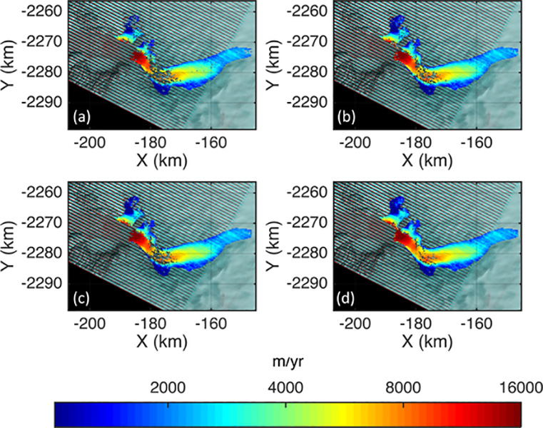
The matching results with the four combinations of the different configurations are illustrated in Fig.6. Unconstrained feature tracking required 537080 seconds to complete all 64 matches for the image pair in Fig.5(a). Application of DLC reduced the processing time to 5983 seconds, which is an improvement by 98.9% compared to the unconstrained matching. The numbers and distribution of correct matches in each case are presented in Table II and in Fig.6. These show that DLC and QM result in increased numbers of correct matches, especially on the cloud-covered area and the bend in flow direction (X=−177km, Y=−2287km) on the main glacier trunk.
Fig.6.
Comparison of feature tracking results from Fig.5(a), overlain on image backgrounds. (a): Original forward matching without DLC, (b): Original forward matching with DLC, (c): QM without DLC, (d): QM with DLC. Note that the speed is plotted in log scale.
Table II.
Ratio of Successful Matching in the ETM+ Pair. The Root Mean Squared Differences are presented at the Second Lines of each Cell.
| Method | Without DLC | With DLC |
|---|---|---|
| Original forward only | 2918/3793 (76.93%)±6.02 (0.16%) | 3418/3793 (90.11%)±14.38 (0.38%) |
| QM | 3300/3793 (87.00%)±8.06 (0.21%) | 3662/3793 (96.55%)±2.49 (0.07%) |
The improvement presented in Fig.6 and Table II is explained by the exclusion of spurious possible NCC peaks that are far off from the expected direction of the flow. The redundancy provided by QM further increases the chances that each grid has at least one correct match beyond what is provided by forward-only matching.
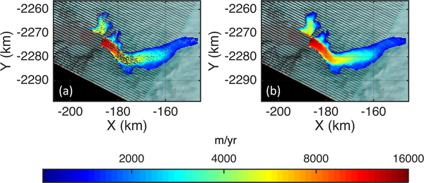
The results of the postprocessing algorithms are presented in Fig.7 and Table III. We find that pseudosmoothing substantially reduces noise when compared to the results obtained from the voting cell method. The results in Table III show that the ratio of successful matches from QM with DLC (4 matching per grid) is only about 3 percent less than that of pseudosmoothing (64 matching per grid). This small difference comes from the nature of manual and automatic postprocessing. The results in Table II are from manual selection of correct displacements from visual inspection, which can be more flexible but time-consuming and impractical to apply to a number of pairs available in the time series. In contrast, pseudosmoothing is a automated postprocessing algorithm, which is faster but can be less flexible than manual filtering.
Fig.7.
Postprocessing results from “voting cell” method (a) and pseudosmoothing method (b).
Table III.
Ratio of Successful Matching after Postprocessing, with Their Root Mean Squared Difference. Their Respective Percentages are presented at The Parentheses in Each Cell.
| Total # grids | Correct matchings | |
|---|---|---|
| Voting-cell | Pseudosmoothing | |
| 3793 | 3041±5.31 (80.17±0.14%) | 3779±2.94 (99.63±0.08%) |
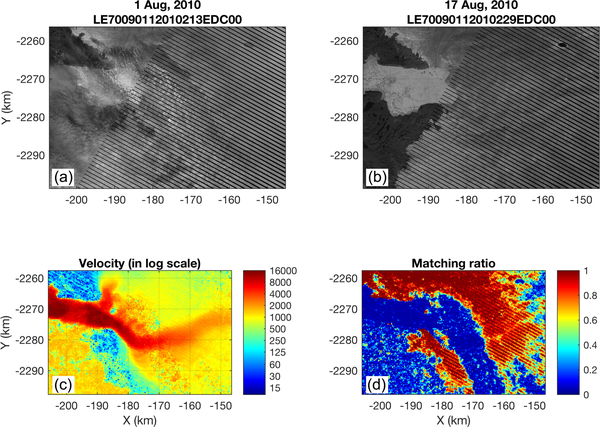
Despite of the robustness of this MIMC algorithm, it is not possible to measure the displacement when the ice surface texture is covered by opaque cloud, resulting in false matches. Such spurious matching can be detected by matching ratio, which is the number of displacements in a valid cluster in each grid divided by total number of matching attempts. A larger ratio means that the feature tracking was more successful and consistent regardless of the MIMC parameters. Fig.8 provides an example of the matching ratio in areas of cloud cover. We find that area with smooth gradients in velocity have relatively high matching ratios. In contrast, speeds in areas of low matching ratio are relatively noisy.
Fig.8.
ETM+ image pairs with thick cloud cover (a, and b) with the obtained speed (c) and matching ratio (d) maps obtained from the pair. The data acquisition date and the scene IDs of the source data are presented at top of the each subset.
The improved performance of pseudosmoothing over the voting-cell approach results from the synergy of several components. First, by applying the filter to clusters of displacements, starting with the most dominant, a consistent, and thus high-confidence result is obtained. If there is no dominant cluster in a grid, the displacement is left blank and passed to the next procedure, rather than filling the grid with less confident and possibly spurious values. Avoiding those less confident displacements from the beginning of the process prevents the propagation of errors through the processing chain. Second, improved post processing is achieved with the use of a priori information to find the most probable clusters of displacements.
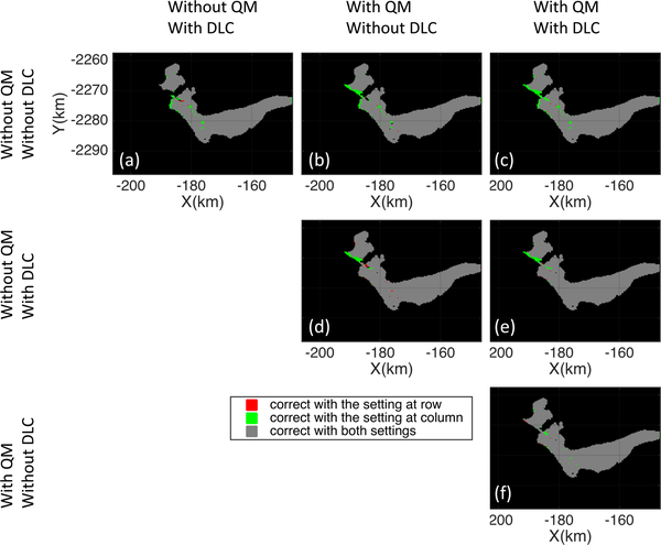
The effects of DM and QLC to the pseudosmoothing results from Fig.5(a) are presented in Table IV and Fig.9. Overall, there were increases in correct matches of 2.21% and 3.24% resulting from QM and DLC, respectively, with their combination resulting in a 4.01% increase. Most of the additional successful matches are obtained from the glacier terminus and shear margins. The increase in success resulting from QM at the terminus is explained by the swapped matching. The ice within reference image chip close to the terminus may reach the calving front and be lost between image acquisitions. Reverse tracking ensures that velocities can be obtained as close as possible to the calving front. The inclusion of DLC is most effective at the shear margins and areas of flow near the terminus where the a priori velocity field reduces the search area and improves the chance of successful match.
Table IV.
Ratio of Successful Matching after pseudosmoothing with and without the QM and the DLC, with Their Root Mean Squared Difference. Their Respective Percentages are presented at The Parentheses in Each Cell.
| Without DLC | With DLC | |
|---|---|---|
| Without QM | 3627±4.32 (95.62±0.11%) |
3710±3.74 (97.81±0.10%) |
| With QM | 3749±4.50 (98.84±0.12%) |
3779±2.94 (99.63±0.08%) |
Fig.9.
Comparison maps of correct matches obtained from postprocessing results of different feature tracking settings. Red dots mean that configuration at the row gave correct matches, whereas the settings at the column was not. Green dots mean vise versa. Gray dots mean both of the two settings were successful.
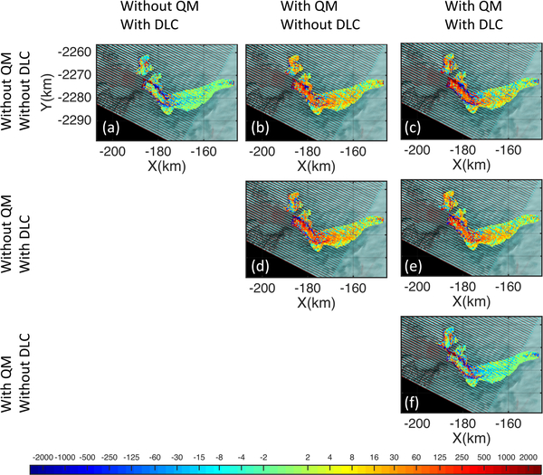
Statistics of the difference in the speeds calculated using each combination of algorithm components are presented in Table V and the spatial distribution is shown in Fig.10. The table tells that the QM has caused about 28m/yr of discrepancy when DLC was not applied, and 45m/yr of difference when DLC was applied. In contrast, DLC has caused about 20m/yr and 19m/yr of discrepancy when QM has turned on and off respectively. Therefore, we find that QM results in more differences than the DLC in the measured velocities. In addition to the biases, the use of QM results in lower speeds over the fast-flowing glacier trunk (Fig.10(b) and (e)). This is due to the velocity gradient along-flow. The glacier’s flow converges at its terminus, causing faster flow speed at its terminus than at the upglacier region. That causes the flow speed increases along the flow, causing positive velocity gradient along the flow direction. That means the displacement measured along the flow direction (i.e. heading the terminus) is usually larger than that measured reverse to the flow (i.e. heading the upglacier region). Since QM performs matching in both the forward reverse directions, a large change in velocity along-flow, as found on the trunk of Jakobshavn Isbræ, will result in substantially difference displacements between the forward and reverse matches, leading to a different final displacement than if QM is not employed.
Table V.
Mean and standard deviations of the velocity differences produced with and without QM and DMC. The first and the second values in each line are x and y components of the velocity. The First and the second line in each cell depicts mean and standard deviation in each MIMC setting. The Unit of all values are in m/yr.
| Method | Without QM With DLC | With QM Without DLC | With QM With DLC |
|---|---|---|---|
| Without QM | (15.09,−13.24) | (−24.18,−15.06) | (36.92,−10.15) |
| Without DLC | (363.01,295.73) | (368.05, 306.37) | (466.23, 274.86) |
| Without QM | N/A | (−37.50, −3.15) | (−44.76, −2.10) |
| With DLC | (421.84,313.10) | (400.37, 274.86) | |
| With QM | N/A | N/A | (−16.87, 9.22) |
| Without DLC | (408.73, 344.60) |
Fig.10.
Speed difference between the measurements obtained from different feature tracking settings. The difference is calculated by subtracting the speed from the settings on column from the settings from the row. The speed difference is colorscaled in log as shown in the colorbar at the bottom.
The pattern of speed difference in Fig.10 tells that the speed difference by QM at the main trunk (Fig.10(b) and (e)) is more visible than that by DLC (Fig.10(a) and (f)). The noisy patterns at the shear margin are found from the figure, which can be explained by feature tracking error caused by the non-transitional distortion of the surface texture. Despite the pattern, the overall difference did not exceed 45m/yr, or 0.13 pixels (Table V).
One concern is that utilizing a priori information in postprocessing may bias the solution toward the a priori, over constraining the solution. However, as per (15), only the a priori displacement direction, and not speed, is used when determining the initial displacement (d2). Moreover, pseudosmoothing iteratively analyzes the smoothness of the neighboring vectors and replaces the initial displacements into the clusters’ displacements. Thus, the determined displacement is not an interpolated value, but is rather the displacement within the cluster that gives the smoothest result.
B. Contribution of the multiple matching components
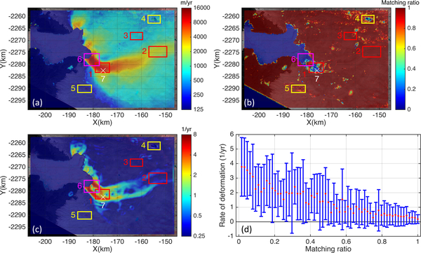
The pseudosmoothed velocity map from the pair shown in Fig.5(b) using the complete algorithm is shown in Fig.11. Using this result, we examine the impacts of high shear strain rates, supraglacial lakes, clouds and motion of the ice front on the results. The maps of matching ratio and the deformation rate (rooted sum of the square of normal and shear strain rates) are also provided in the figure. We find consistently high matching ratios with anomalies over the lower region of the main trunk, below the bend in flow (region 6 and 7 in the figure), and in the vicinity of a supraglacial lake (area 4).
Fig.11.
(a): Speed map derived from an image pair in Fig.5(c), (b): Matching ratio, (c): deformation rate map with the Gaussian filter applied, and (d): Distribution of deformation rate with respect to matching ratio. Note that the log color scales have applied for (a) and (c), and that Gaussian filter was applied on (c).
We first consider the impact of high shear strain rates. The deformation rate map in Fig.11(c) derived from the velocity field in Fig.11(a) shows high shear strain rates in the middle of the main trunk, where the direction of flow changes by about 45 degrees. The matching ratio degrades substantially over the areas with larger shear strain rates. This trend is plotted in Fig.11(d).
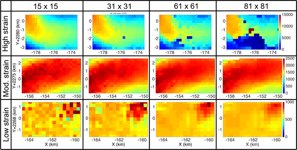
To investigate the cause for the decrease in matching ratio with increasing shear strain rate, we applied the multiple matching algorithm by confining the size of reference chip into single value, while fully utilizing different image filters and components in QM. Constrained multiple matches were performed with the reference chips sizes given in section II-E. Zoomed-in results for the regions of low, moderate and high shear indicated in Fig.11 are presented in Fig.12. From those results, we find that the smaller reference chip is more successful for finding a matching point than the larger chip in areas of higher shear strain. In contrast, the results of the moderate and low strain areas get smoother as the chip size grows.
Fig.12.
Results from multiple matching over regions of differing shear strain rate with differing reference chip sizes. Each row is results from the high, moderate and low strain areas shown in Fig.11, box 1,2, and 3 respectively. Each column is the result obtained using reference chip sizes of 15 by 15, 31 by 31, 61 by 61 and 81 by 81 pixels, respectively.
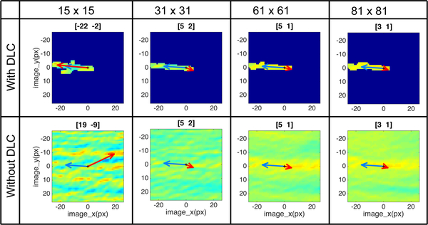
Typically, the use of the small reference chip for NCC-based tracking is problematic on glaciers due to ambiguities arising from repetitive textures, such as crevasses, resulting in spurious matches. Larger reference chip sizes can avoid this ambiguity. However, the significant geometric distortion of the surface texture in areas of high shear strain rates may result unsuccessful or incorrect matches with larger chip sizes. In this situation, DLC effectively reduces the chance of encountering ambiguous textures, allowing for smaller reference chips, and thus less sensitivity to the textures’ shape deformation. This is demonstrated for a point of high shear strain (point 7 in Fig.11(a)) presented in Fig.13. Out of the range of chip sizes used, the smallest reference chip (15 by 15 pixels) with DLC gave the highest confidence displacements. In contrast, larger chip sizes resulted in spurious matches (i.e. direction opposite to InSAR flow direction). Without DLC, for the same point, a 15 by 15 reference chip also resulted in a clearly spurious result due to textural ambiguity. Without DLC, larger chip sizes resulted in the same, spurious displacements. This supports the effectiveness of DLC in improving measurements in areas of high shear through the use of smaller reference chip sizes.
Fig.13.
Normalized Cross-Correlation (NCC) maps for location 7 in Fig.11, with different reference chip sizes and with and without (DLC). Blue arrows are expected displacement derived from the InSAR velocity data, and red arrows are feature tracking results, i.e. the NCC peaks for each case. The relative locations of the NCC peaks are presented on top of each plots in the precision of integer. Dark blue areas in the DLC results mean that NCC was not calculated.
In addition to the ability of finding the correct matches, Fig.13 provides evidence about the faster NCC peak search discussed in II.B. The dark blue areas in the NCC maps with DLC in the figure are the points for which NCC was not calculated because they were outside the spatial constraint imposed by the DLC. The drawback of null exclusion NCC calculation [11] is that the computation is performed in spatial domain, so that the effective calculation in frequency domain is not possible [12]. However, DLC optimizes the amount of computation by reducing the spaces to calculate the NCC, so that the NCC peak location can be found in faster manner.
While smaller reference chips improve measurements over areas of high strain rates, Fig.12 also demonstrates that larger chip sizes provide smoother results over areas of low to moderate shear. In those areas, the advantage of a small reference chip decreases because shape distortion and rotation is less. There, larger reference chips are more statistically stable because more samples are used to calculate the NCC peak. Thus, we find a complimentary benefit to smaller and larger reference chip sizes as dependent on shear strain rate.
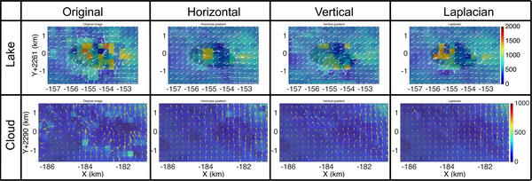
For features such as clouds and supraglacial lakes, the image filters applied in the multiple matching scheme are critical. In this study, feature tracking was applied to horizontal gradient, vertical gradient, and Laplacian filtered images, as well as the unfiltered images. Fig.14 compares the postprocessed results for areas with a supraglacial lake and partial cloud cover obtained from the original and filtered images. In both cases, the number of spurious matches decreases and the number of likely correct matches increases when using the filtered imagery.
Fig.14.
Pseudosmoothing results with different image filters for areas indicated in Fig.10. The results from supraglacial lake (box 4 in Fig.11) are in the upper row and the ones from cloud cover (box 5 in Fig.11) are in lower row. The color-coded velocities are in unit of m/yr.
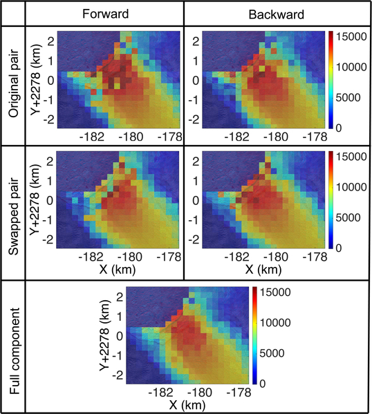
Finally, glacier calving fronts are problematic for RIFT methods because they can advance or retreat between image pairs and features upglacier of the front in the first image may advect through the front (and calve) in the second image, causing a data gap near the front. These problems were mitigated by QM, as shown in Fig.15. By swapping the pairs, features at the front are tracked in reverse, resulting in displacement measurements up to the front. Further, we see that the individual match iterations within the QM sequence are noisy, potentially due to variations in glacier front position that contaminate the flow field. However, the combination of the four iterations results in a high confidence and smooth displacement field.
Fig.15.
Pseudosmoothing results near a calving front (box 6 in Fig.11(a)) for multiple matches using the different components of QM. The maps in the first row are from original pairs while those in the second row are from the swapped pair. The results in the first column are from forward matching while those in the second column are from backward matching. The map in the third row is obtained from the full QM procedure.
IV. Conclusion
Comparative studies of RIFT algorithm performance have shown that all provide similar results using cloud-free and well-contrasted imagery over textured terrain, with some algorithms performing better in specific cases. The current challenge, therefore, is to develop improved algorithms for efficiently processing large datasets of varying image quality and terrain types. Here, we build upon the multiple image approach of [7] by introducing multi-directional matching, termed Quadramatching, and incorporate a priori velocity information to constrain both the match direction (Dynamic Linear Constraint) and postprocessing (Pseudosmoothing). We demonstrated that these modifications substantially improved the number and quality of displacement measurements over the previous algorithm. We also found that the improvement provided by the new algorithm was achieved by (1) creating a positive, complementary effect between reference chip size and DLC and (2) by adding sample redundancy in displacement generation.
The major disadvantage of this algorithm is the increase in processing time. Despite the reduction in search space provided by DLC, the expanded multiple match approach increases the total amount of calculation. This could be mitigated by identifying and removing combinations of window sizes, image filters and search directions in the multiple matching scheme that do not improve the final result. Finally, the clustering result used in the pseudosmoothing processing can be sensitive to the given threshold (ρmin). Future work should be directed at finding an adaptive threshold to further improve the generality and robustness of the algorithm.
Acknowledgments
The work was supported by grant NNX10AN61G to I.M.H. from the U.S. National Aeronautics and Space Administration.
Biography
 Seongsu Jeong received B.Sc. and M.Sc. in Civil and Environmental engineering degree in 2008 and 2010 respectively from Yonsei University, Seoul, Korea, and Ph.D. degree in geodetic science from The Ohio State University, Columbus Ohio. He is currently a postdoctoral researcher in Byrd Polar and Climate Research Center at The Ohio State University, Columbus. His research topic includes feature tracking, optical remote sensing and glacier dynamics. Dr. Jeong is a member of the American Geophysical Union.
 Ian M. Howat received the B.A. degree in geology from Hamilton College, Clinton, NY, in 1999 and the Ph.D. degree in earth science from the University of California, Santa Cruz, in 2006.
He is currently an Associate Professor with the School of Earth Sciences, The Ohio State University, Columbus. His research focuses on observing and modeling ice sheet and glacier dynamics.
Dr. Howat was the recipient of the U.S. Presidential Early Career Award for Scientists and Engineers in 2011. He is a member of the American Geophysical Union and the International Glaciological Society.
 Yushin Ahn received the B. Eng degree in Civil engineering and the M.S degree in surveying and digital photogrammetry from Inha University, Inchun, Korea in 1998 and 2000, respectively, and the M.Sc. And Ph.D. degrees in geodetic science from Ohio State University, Columbus, in 2005 and 2008, respectively.
Dr. Ahn is currently an Assistant Professor in Surveying Engineering and Integrated Geospatial Technology Program, Michigan technological University, Houghton. His research focuses on digital photogrammetry, feature tracking and sensor calibration and integration. He is a certified Photogrammetrist and a recipient of the Robert E. Altenhofen Memorial Scholarship from American Society of Photogrammetry and Remote Sensing.
Contributor Information
Seongsu Jeong, Byrd Polar and Climate Research Center, The Ohio State University, Columbus, OH 43210 USA.
Ian M. Howat, School of Earth Sciences, The Ohio State University, Columbus, OH 43210 USA
Yushin Ahn, School of Technology, Michigan Technological University, Houghton, MI 49931 USA.
References
- [1].Joughin I, “Ice-sheet velocity mapping: a combined interferometric and speckle-tracking approach,” Ann. Glaciol, vol. 34, pp. 195–201, 2002. [Google Scholar]
- [2].Joughin I, Smith BE, Howat IM, Scambos T, and Moon T, “Greenland flow variability from ice-sheet-wide velocity mapping,” J. Glaciol, vol. 56, no. 197, pp. 415–430, 2010. [Google Scholar]
- [3].Rignot E, Mouginot J, and Scheuchl B, “Ice Flow of the Antarctic Ice Sheet,” Science, vol. 333, no. 6048, pp. 1427–1430, September 9, 2011. [DOI] [PubMed] [Google Scholar]
- [4].Skvarca P, Raup B, and Angelis H. d., “Recent behaviour of Glaciar Upsala, a fast-flowing calving glacier in Lago Argentino, southern Patagonia,” Ann. Glaciol, vol. 36, pp. 184–188, 2003. [Google Scholar]
- [5].Berthier E, Raup B, and Scambos T, “New velocity map and mass-balance estimate of Mertz Glacier, East Antarctica, derived from Landsat sequential imagery,” J. Glaciol, vol. 49, no. 167, pp. 1–9, 2003. [Google Scholar]
- [6].Howat IM, Box JE, Ahn Y, Herrington A, and McFadden EM, “Seasonal variability in the dynamics of marine-terminating outlet glaciers in Greenland,” J. Glaciol, vol. 56, no. 198, pp. 601–613, 2010. [Google Scholar]
- [7].Lee H, Shum CK, Howat IM, Monaghan A, Ahn Y, Duan J, et al. , “Continuously accelerating ice loss over Amundsen Sea catchment, West Antarctica, revealed by integrating altimetry and GRACE data,” Earth Planet. Sci. Lett, vol. 321-322, pp. 74–80, 2012. [Google Scholar]
- [8].Paul F, Bolch T, Kääb A, Nagler T, Nuth C, Scharrer K, et al. , “The glaciers climate change initiative: Methods for creating glacier area, elevation change and velocity products,” Remote Sens. Environ, vol. 162, pp. 408–426, 2015 [Google Scholar]
- [9].Jeong S and Howat I, “Performance of Landsat 8 Operational Land Imager for mapping ice sheet velocity,” Remote Sens. Environ, vo. 170, pp. 90–101, 2015. [DOI] [PMC free article] [PubMed] [Google Scholar]
- [10].Fahnestock M, Scambos T, Moon T, Gardner A, Haran T, and Klinger M, “Rapid large-area mapping of ice flow using Landsat 8,” Remote Sens. Environ, In press. [Google Scholar]
- [11].Ahn Y, and Howat IM, “Efficient Automated Glacier Surface Velocity Measurement From Repeat Images Using Multi-Image/Multichip and Null Exclusion Feature Tracking,” IEEE Trans. Geosci. Remote Sens, vol. 49, no. 8, pp. 2838–2846, 2011. [Google Scholar]
- [12].Warner RC, and Roberts JL, “Pine Island Glacier (Antarctica) velocities from Landsat7 images between 2001 and 2011: FFT-based image correlation for images with data gaps,” J. Glaciol, vol. 59, no. 215, pp. 571–582, 2013. [Google Scholar]
- [13].Lewis JP, “Fast Normalized Cross-Correlation,” presented at the Vision Interface, 1995. [Google Scholar]
- [14].Scambos TA, Dutkiewicz MJ, Wilson JC, and Bindschadler RA, “Application of Image Cross-Correlation to the Measurement of Glacier Velocity Using Satellite Image Data,” Remote Sens. Environ, vol. 42, pp. 177–186, 1992. [Google Scholar]
- [15].Fallourd R, Vernier F, Friedt J-M, Martin G, Trouvé E, Moreau L, and Nicolas J-M, “Monitoring temperate glacier with high resolution automated digital cameras–application to the Argentière Glacier,” Int. Arch. Photogram. Remote Sens. Spatial Inf. Sci, vol. 38, pp. 19–23, 2010. [Google Scholar]
- [16].Whillans IM and Tseng Y-H, “Automatic tracking of crevasses on satellite images,” Cold Reg. Sci. Technol, vol. 23, pp. 201–214, 1995. [Google Scholar]
- [17].Scherler D, Leprince S, and Strecker MR, “Glacier-surface velocities in alpine terrain from optical satellite imagery - Accuracy improvement and quality assessment,” Remote Sens. Environ, vol. 112, pp. 3806–3819, 2008. [Google Scholar]
- [18].Heid T, and Kääb A, “Evaluation of existing image matching methods for deriving glacier surface displacements globally from optical satellite imagery,” Remote Sens. Environ, vol. 118, pp. 339–355, 2012. [Google Scholar]
- [19].Kääb A, “Monitoring high-mountain terrain deformation from repeated air- and spaceborne optical data: examples using digital aerial imagery and ASTER data,” ISPRS J. Photogramm. Remote Sens, vol. 57, pp. 39–52, 2002. [Google Scholar]
- [20].Kääb A, “Combination of SRTM3 and repeat ASTER data for deriving alpine glacier flow velocities in the Bhutan Himalaya,” Remote Sens. Environ, vol. 94, pp. 463–474, 2005. [Google Scholar]
- [21].Irons JR, Dwyer JL, and Barsi JA, “The next Landsat satellite: The Landsat Data Continuity Mission,” Remote Sens. Environ, vol. 122, pp. 11–21, July 2012. [Google Scholar]
- [22].Joughin I, Smith B, Howat I, and Scambos T (2011), updated 2014 MEaSUREs Greenland Ice Velocity: Selected Glacier Site Velocity Maps from InSAR. W69.10N. Boulder, Colorado USA: NASA DAAC at the National Snow and Ice Data Center; Available: 10.5067/MEASURES/CRYOSPHERE/nsidc-0481.001. [DOI] [Google Scholar]


